Article

Methods for Distributed Compressed Sensing

School of Electrical Engineering and ACCESS Linneaus Centre, KTH Royal Institute of Technology, Stockholm SE-100 44, Sweden
*
Author to whom correspondence should be addressed.
J. Sens. Actuator Netw. 2014, 3(1), 1-25; https://doi.org/10.3390/jsan3010001
Submission received: 15 October 2013 / Revised: 29 November 2013 / Accepted: 9 December 2013 / Published: 23 December 2013
(This article belongs to the Special Issue Feature Papers)

Abstract

:
Compressed sensing is a thriving research field covering a class of problems where a large sparse signal is reconstructed from a few random measurements. In the presence of several sensor nodes measuring correlated sparse signals, improvements in terms of recovery quality or the requirement for a fewer number of local measurements can be expected if the nodes cooperate. In this paper, we provide an overview of the current literature regarding distributed compressed sensing; in particular, we discuss aspects of network topologies, signal models and recovery algorithms.

1. Introduction

With the increased availability of cheap sensors, applications with sensor networks are of major interest to the community. In such networks, data signals (possibly correlated) are gathered by sensors and processed either distributively (at the local sensor nodes) or at some fusion center (centralized). Natural signals are often compressible; a signal may be of a large dimension, but the information content is small. Instead of collecting such large signals, fewer measurements can be used to reconstruct the signal. To this end, compressed sensing (CS) [1,2] has been an active research area over the past few years. CS relies on few random measurements being sufficient to reconstruct a large signal where the information content is sparse. Comparing CS to traditional data compression systems, the complexity is moved away from the information source, and instead, we find a challenge in the signal reconstruction part of the system. Two main classes of reconstruction methods are dominant; the convex relaxation-based solvers in which a relaxed problem is solved exactly, and the greedy pursuit (GP)-based solvers in which the exact problem is solved sub-optimally.
In a CS system, if signals measured at different sensors are correlated, the necessary number of measurements can be further reduced by exploiting correlations in the reconstruction process. Therefore, we have recently seen a growing interest in different attempts to improve CS performance by designing new reconstruction algorithms for multiple signals. For such problems, which we refer to as distributed compressed sensing (DCS) problems, there are few specific analytical results available. For the results that are available, the gap between what is practically achieved and the prediction of the analytical result is often large; which is true already at the single sensor setting [3]. We endeavor to provide a moderate level of overview on practical DCS algorithms. The paper is arranged by first a description of DCS problems (Section 2) along with fundamental tools for relevant mathematical justifications, basic types of networks considered in the literature where DCS can be realized (Section 3), various signal models for data correlation (Section 4), several convex relaxation-based approaches to DCS problems (Section 5) and, finally, GP algorithms for DCS problems (Section 6). Finally, we also provide some simulation results and a reflection on the performance criteria for evaluating DCS (Section 7).

1.1. Notation

A vector is lower-case bold-face, for example, x ; matrices are upper-case bold-face, for example, A . We denote the matrix transpose, A T , and pseudo-inverse, A . For a sparse signal, x , we collect the indices of the non-zero components in the support set, which is denoted with calligraphic letters T , but we also use I and J for this purpose. To describe the sensor node in a network, we use the calligraphic set, L , to represent the nodes in the network. We will use the 1 and 2 -norm, but we also define the zero-norm as a counter · 0 : = { number of nonzeros } . We denote expectation by E .

2. Distributed Compressed Sensing Setup

We define the distributed compressed sensing (DCS) setup as a multiple-node extension to the standard CS setup. In the case of only one single node in the network, the DCS setup reduces to the standard one-sensor CS setup. Let y l R m l be a measurement vector observed in node l by the following linear system:
y l = A l x l + e l l L
Here, A l R m l × n is a measurement matrix through which we observe the signal vector, x l R n ; e l R m l is measurement noise, and L is the set of nodes present in the network. If nothing else is stated, we assume that the measurement-matrix, A , is constructed by choosing each matrix-component from a standard independent, identically distributed (i.i.d.) Gaussian source and then normalize the matrix column-wise to unit 2 norm. In the DCS setup, x l is a sparse signal, meaning that the number of non-zero components in x l is small. We let x l 0 = s l be the number of non-zero components in the vector. In DCS, we assume that s l < m l < n . Furthermore, we can collect the non-zero indices (or atoms) in x l and put these in a set, which we call a support-set. The support-set for x l is denoted by l = { i : x l ( i ) 0 } . Using the support-set, we can form the s l -sized dense vector, x T l , which contains only the non-zero values of x l . Similarly, we can collect the columns in A l corresponding to the active components in the m l × s l -sized matrix A T l . Here, we mention that A l x l = A T l x T l .
In the DCS setup Equation (1), the sparse assumption of the measured signal, x l , may seem artificial. The natural signal that is being measured may instead be a non-sparse signal z l = Φ l x l , where Φ l represents some transform to another domain (i.e., using the Fourier transform to the frequency domain). The important property for the measurement matrix is incoherence, a property fulfilled by, for example, matrices with Gaussian zero mean i.i.d. components. Thus, we can form the new transformation matrix B l = A l Φ (still Gaussian i.i.d.). Using this notation, we can find z l from x l by Φ 1 x l . In general, we know a transformation, Φ, where the signal is strictly, or approximately, sparse. An approximately sparse signal has a major part (say, 95%) of its energy located in only a few (say s l ) components. In this article, we will always attempt to find the solution to Equation (1) assuming that x l is sparse directly in a Euclidean basis. We do not emphasize how to treat approximately sparse signals.
In the DCS problem, we are typically interested in improving the recovery accuracy of x l , or the requirements on the measurement device, compared to the single-sensor case by assuming that the data among sensor nodes in a network are correlated. The idea is then that by collecting, or sharing, some information among the nodes and exploiting this correlation, we can achieve better performance. The signal correlation is usually modeled differently depending on the application; we will model correlations by signal models in Section 4. To understand the procedure of DCS solvers, we first give a description of the standard (single node) CS problem. When we later introduce the DCS solvers, we will also provide examples of single-sensor CS solvers.

2.1. Single Node Reconstruction Problem

For the single node reconstruction, we drop the subscript, l. We then have y = A x . Given y and A , the CS reconstruction problem is to find the sparse vector, x . Note that if x had not been sparse, our task would have been impossible, since the system is underdetermined. However, assuming that x is sparse, we can instead attempt to find a solution to the following problem:
min x ^ x ^ 0 such that y A x ^ 2 ϵ
The above problem is, in general, non polynomial hard (NP-hard) and is, thus, not usually considered in practice. As mentioned in the Introduction, the two main approaches to solving Equation (2) are either to form a convex relaxation to relax the non-convex zero norm and solve a convex problem (Section 5) or to approximately solve Equation (2) with some GP algorithm (Section 6).
For the CS problem, there are some fundamental mathematical tools specifying the conditionality of the measurement matrix. These tools are traditionally used to determine the reconstruction performance of a CS solver.
Definition 1 (RIP: Restricted Isometry Property [4]) 
A matrix, A , satisfies the RIP with Restricted Isometry Constant (RIC) δ s if:
( 1 δ s ) x 2 2 A x 2 2 ( 1 + δ s ) x 2 2
for all s-sparse vectors x where 0 δ s < 1 .
We note that in the literature, there are various other interesting properties that can be applied in the CS setup. For example, we mention mutual coherence [5], the restricted nullspace condition [5,6,7] and the restricted eigenvalue condition [8]. These bounds are less restrictive than the RIP and may be well suited for performing sufficient condition guarantees; however, they are presently not as commonly used as the RIP in algorithm analysis.

2.2. Distributed Setups vs. Distributed Solvers

In DCS problems, there is an immediate risk of confusion between two concepts: distributed setups and distributed solvers. The first concept regards the setup where different sensors in a network collect data, which is correlated among the sensor nodes. We refer to this as distributed CS setup (DCS setup), where the correlation is modeled with some signal model, discussed in Section 4. The second concept regards solving either the standard CS or the DCS, by utilizing several computational nodes. The computational nodes may be distributed in a network (see Section 3) or locally placed within a multiple core processor, and we refer to such a solver as a distributed CS solver (DCS solver). In this article, we focus on the DCS setups, as well as DCS solvers. Generally, in DCS problems, it is of interest to minimize both computational cost and communication overhead; in turn, transmitting little information and using efficient algorithms.

3. Network Models

A network is an infrastructure where data is shared through connections between different sensing and/or computational nodes. For analysis of distributed algorithms, the choice of network model plays an important role. Some models closely resemble practical random networks, while others are fixed and structured to provide controlled performance comparison. If every node in a network can transmit information to every other node through one or multiple hops, the network is said to be connected. If there is a direct link between every node in the network, the network is said to be fully connected. If no connection can be found between two nodes (either directly or through multiple hops), the network is disconnected, and then, we can regard the nodes as forming two or more independent networks.
Formally, we say that sensor node l has a set of neighbors to which it can transmit information (outgoing set of neighbors), defined as L l out , and a set of incoming neighbors (from which it receives information), defined as L l in . These sets are not necessarily the same, implying that all connections are not two-way. We also define a complete network with all nodes as L . To model networks, there are two main categories of network models: fixed network models and random network models. The fixed network models are completely determined, while the random networks have some parameters determining a random layout. We will discuss both types of network models and start with the fixed ones.

3.1. Fixed Network Models

In a fixed network, the connections among the sensor-nodes are manually formed. For example, we can imagine sensors equidistantly aligned horizontally and vertically to form a lattice, as in Figure 1a. This may closely model the connections formed by independent sensors placed uniformly over some area. Observe that the network connections can be formed this way, even when the sensors are spatially located according to some other topology. In the task of analyzing the performance of DCS algorithms, this fixed network model may not be the best suited one, since it is hard to understand how to modify the network connectivity.
Figure 1. Lattice and circular network topologies.
Jsan 03 00001 g001
The forward circular network model in [9] is an example of a fixed network that is designed specifically to make modifications of connectivity easily amenable. In this network model, nodes are artificially placed in a circle, and connections among the nodes are realized by one-way communication links. The network having the least possible connections, such that it is fully connected, is thus formed by letting each node connect to one other node according to Figure 1b. By forming this circular topology of nodes and forwardly adding new connections in a systematic way, we can study how the overall performance of an algorithm improves as the network connectivity increases. In Figure 1c, we show a network where each node is connected to two other nodes (referred to as a degree two network). By adding more connections according to the forward circular model, we can, in a controlled manner, systematically improve the connectivity until the network is fully connected (where each node is connected with every other node). Another common circular network topology approach is to allow for bidirectional communication links, and we refer to such a model as a circular network model (compared to the previous forward circular network model). In Figure 1d, we see a typical example of a standard circular network model based on bidirectional connections.

3.2. Random Network Models

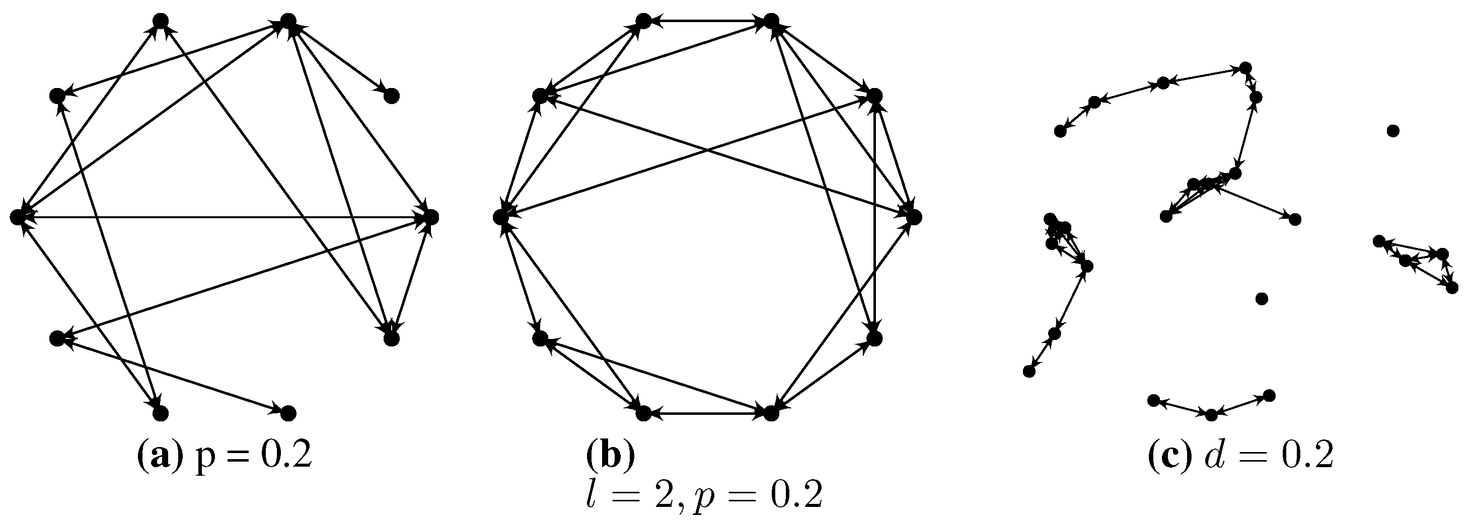
When the setup grows large and the focus is on practical applications, the category of random network models may be of more relevance. Of several popular random models, we first present the random graph network model developed by Erdős and Rényi in [10]. Erdős and Rényi take an analytical approach, deriving probabilities for full network connectivity and connectivity distributions for the nodes. From an engineering perspective, we can utilize their model to generate a network based on a parameter, p, which specifies the probability that any two nodes are connected. An example of the random graph network model with probability parameter p = 0 . 2 is shown in Figure 2a. Note that the circular placement of the nodes has nothing to do with the topology of the connections. A (semi-)random network model utilizing two tuning parameters, l and p, was presented by Watts and Strogatz in [11]. The first tuning parameter, l, specifies that each node in the network should be connected with l neighbors structurally (i.e., as in the forward circular model). Then, with probability p, each such connection is rewired to another node, where the other node is chosen uniformly at random. This model has the strength that if p = 0 , it represents a completely structured model, and if p = 1 , it represents a (uniformly) random model. Thus, this network model may be suitable for understanding how a system behaves for the intermediate networks. We show an example of the Watts–Strogatz network model in Figure 2b for ten sensor nodes, where l = 2 and p = 0 . 2 . In the random geometric graph model, presented by Penrose in [12], nodes are placed randomly (according to some distribution) within a unit-length square. Then, every node connects with every other node located within distance d of it. We show an example of such a network in Figure 2c. Here, the distribution chosen is uniform, and we have chosen d = 0 . 2 . Any of these three random models may lead to disconnected networks.
Figure 2. Random network topologies.
Jsan 03 00001 g002
The network models we have mentioned are general in the sense that they are not intentionally created to model a specific application. We notice that in the literature, there are many examples of such specific network models. One such example is presented in [13] by Barabási and Albert, which models hyper-link connections on the Internet.

3.3. A Comment on Fundamental Limits in Networks

In a sensor network, assume nodes 1 and 2 want to communicate some information and we are interested in the maximum rate at which communication can take place. If finding the precise rate between the nodes is not possible, we can still upper-bound it using the max-flow min-cut theorem [14,15]. By cutting the network into two parts, so that the first node resides in one part and the second node in the other part, and assuming full cooperation within the parts, we can find the maximum communication rate between these two parts. If we derive the rate for all possible cuts in the network (such that node 1 is in one part and node 2 in the other), we get max-flow min-cut rate as the smallest such rate. Precisely, the max-flow min-cut rate is an upper bound to the maximal possible rate (or flow) with which two nodes can communicate in a network.
Information theory provides sufficient conditions for information exchange, while we, for compressed sensing in networks, are still searching for necessary conditions on the CS part of the problem; therefore, a common assumption is often that the transmission links are perfect (but maybe costly). There has been some attempts at bringing information theory and compressed sensing together [16,17,18]. In our understanding, if information theory is brought into DCS, it is also necessary to consider the effects of source and channel coding errors [19,20,21,22,23,24]. We will not consider information theoretic aspects in this article, but instead, we take a prevalent approach, providing performance bounds (upper bounds) in terms of RIP.

4. Signal Models

By exploiting correlation among the data collected by sensor nodes in a network, the challenge in DCS is to utilize this correlation, so that the quality of the locally reconstructed signals improve compared to the disconnected case. In the literature, there are a number of approaches on how to model this correlation; we will enlist several of them here. In general, all these models fundamentally consider the measured signal x l to consist of two parts. One part is individual (private) for the node and the other is joint (common) among all nodes:
x l = i l + j l , l L
where i l is an s i , l -sparse signal component with support-set I l and j l is an s j , l -sparse signal component with support-set J l . In Equation (4), we say that i l is the individual signal component, completely independent among all nodes; and j l is the joint signal component, in some sense, correlated among the sensor nodes. In the remainder of this section, we will discuss more precisely how these components are used in different signal models.

4.1. Common Signal Model

The common signal model assumes that all nodes measure the same signal. This implies that in Equation (4), i l = 0 and j l = j . The model thus becomes:
x l = j , l L
Observe that although the signal we want to measure is identical at all sensors, the measurement devices at the sensors may have different under-sampling and noise properties. Some examples of real-life applications where this model can be used may be seismic activity monitoring, where all sensors measure the same seismic activity; or for a distributed target localization [25], where several sensors cooperate to find the location of a target.

4.2. Mixed Signal Model

The mixed signal model proposed in [26]—where it is also called joint signal model 1 (JSM1)—is a natural extension of the common signal model that allows for individual components, in addition to the joint signal component. Thus, we let j l represent a signal shared among the nodes and j l = j , l and i l represent the individual signal component for each node:
x l = i l + j , l L .
Since this model generalizes the common signal model (by setting i l = 0 l , it reduces to the common signal model), any application in the previous model may also be applicable for this.

4.3. Extended Mixed Signal Model

An extension to the mixed signal model is presented in [27]. Here, subsets of sensors in the network share a joint signal. To describe this model, we use an example from [27]. Let the network consist of three nodes L = { 1 , 2 , 3 } , and the signal of first node is:
x 1 = j { 1 , 2 , 3 } + j { 1 , 2 } + j { 1 , 3 } + i 1
In Equation (7), j { 1 , 2 , 3 } is a set that is shared among all sensors, while j { 1 , 2 } and j { 1 , 3 } are sets only shared among users 1 , 2 and 1 , 3 , respectively. Since the extended mixed signal model is a generalization of the mixed signal model, it can be used in any of the aforementioned scenarios.

4.4. Common Support-Set Model

The common support-set model is sometimes also referred to as the multiple measurement vector (MMV) model, or JSM2:common sparse support-set model [26]; the model states that all sensors measure different signals, but all the signals share the same support-set. Thus the model is:
x l = j l , l L
where the support-set, J l , is shared, so that J l = J , l L . Note, although J is the same for all sensors, the corresponding non-zero values of j l are still individual and possibly independent among the nodes.
An example where this model can be used is for power spectrum estimation [28] in sensor networks. At different locations, the same frequency bands may be occupied (from, e.g., a TV broadcast station), but due to the surrounding scattering and fading, such as buildings, trees, cars, etc., the signal power for each frequency band may be different.

4.5. Mixed Support-Set Model

A natural extension to the common support-set model is the mixed support-set model, proposed by us in [9]. The non-zero components of j l are individual for each sensor, but the locations (i.e., the support-set) of them J l = J l L are the same (joint); the signal values of j l may or may not be correlated. Additionally, there is an individual part, i l , which is completely independent among the sensors, both the support-set and signal values. The model can thus be written as:
x l = j l + i l , l L
An example where this model is suitable is the same power spectrum example for the previous model [28], multiple sensor image acquisition, where each node observes the same object from slightly different angles [29]. For image acquisition, several features from each sensor will be shared, but as each camera has an independent view, completely new features may also appear, from, for example, around corners or behind obstacles. In a similar way, we can also consider multiple sensor sound capturing [30]. Further, the mixed support-set model can be used for a slowly varying signal over time and space.

4.6. Mixed Support-Set Model with Correlations

In the common and mixed support-set model, the signal measured by the sensors share a support-set part, but the signal values are individual. These individual signal values may be chosen as completely independent, but they may also be correlated with an arbitrary correlation parameter, such that E ( j p j q * ) = ρ I N (for p q ), where E denotes the expectation. This mixed support-set model with correlations was proposed by us in [31], but with i p = 0 . Notice that when ρ = 0 , we get the previously defined mixed support-set model, and when ρ = 1 , we get the mixed signal model.

4.7. Common Dense Signal Model

In the common dense signal model presented in [26] (referred to as JSM3), all sensors share a non-sparse joint component | J | = N .
x l = j + i l , l L
In order to extract some data based on this model, the joint, non-sparse part of the signal has to be removed to apply the CS reconstruction algorithms. One example where this model is useful may be in a surveillance camera. In the captured video, each photo might not be sparse, but we may only be interested in detecting movements. By deriving the difference between consecutive photos, we are effectively canceling out static parts, leaving us with sparse signals characterized by movements as sequential changes.

4.8. Limitations in the Signal Models

In general, it is desirable to construct a DCS solver that, based on the most general signal model, performs as well as possible. We expect that solutions tailored to a specific model can provide better performance. In our opinion, the arrangement of most restrictive to least restrictive can be as follows: common signal model, mixed signal model, common support-set model, mixed support-set model and mixed support-set model with correlations. The extended mixed signal model is not practically amenable to use, and the common dense signal model is difficult to handle using the notion of sparsity.

5. Convex Solvers for DCS

In this section, we begin by describing the single node CS convex solver; then, we proceed to DCS problems. We have already observed that the zero-norm in optimization problem (2) is inconvenient, since it is non-convex. Using the current form, there are, in general, no tools available to solve such problems in polynomial time. A possible approach to get around this issue is to relax the problem into a convex one, for example, by replacing the zero-norm with the 1 -norm:
min x ^ x ^ 1 such that y A x ^ 2 ϵ
where ϵ e 2 . It was shown by Candés in [32] that Equation (11), which is called basis pursuit denoising (BPDN), provides robust performance if the measurement matrix is well conditioned. Here, the conditioning of the measurement matrix is expressed in terms of the RIC (see Definition 1); for example, some conditions for robust performance are δ s + δ 2 s + δ 3 s < 1 [4] or δ 2 s < 2 1 [33]. Using the Lagrangian unconstrained form, known as the least absolute shrinkage and selection operator (LASSO) approach, we can solve:
min x ^ λ x ^ 1 + 1 2 y A x ^ 2 2
To solve either Equation (11) or (12), we can use a variety of well-known convex solvers, for example 1 -magic toolbox, CVX (convex toolbox), Sparselab, etc. For sparse signals, the error of the final result, x ^ , of BPDN can be bounded by the following theorem provided by Candés in [32] and by Davenport et al. [34].
Theorem 1 (Theorem 1 in [34]) 
Suppose that A satisfies the RIP of order 2 s with RIC δ 2 s < 2 1 . Given measurements of the form y = A x + e , where e 2 ϵ , the solution x ^ to Equation (11) obeys:
x ^ x 2 C 0 ϵ + C 1 x x s 1 s
where:
C 0 = 4 1 + δ 2 s 1 ( 1 + 2 ) δ 2 s C 1 = 2 1 ( 1 2 ) δ 2 s 1 ( 1 + 2 ) δ 2 s
Note that the 1 -term in the expression provides a component to the bound when the signal is approximately sparse. In most cases, where a result on strictly sparse signals exists, a result on approximately sparse signals can be achieved. We will focus on the strictly sparse signals and refrain from discussing the approximately sparse ones.
For distributed convex solvers, to a centralized problem, first observe that since Equation (11) (or Equation (12)) now is a convex problem (which has been studied for many years), there is a vast convex literature to go through to cover all possible distributed algorithms. One recent work [35] is the alternating direction method of multipliers (ADMM). In short, ADMM is a method that solves (by applying the method of multipliers and one loop of the Gauss–Seidel) the following problem (an example from [25]): Let f and g be two real-valued convex functions and X and Y two polyhedral sets. Let A and B be two full column-rank matrices, and consider the problem:
min x X , y Y f ( x ) + g ( y ) subject to A x + B y = 0
Another approach to develop a distributed convex solver for a centralized problem is based on the simplex algorithm [36]. There are several examples where the simplex algorithm is implemented as a distributed algorithm to be solved in connected networks [37,38,39,40]. However, none of these contributions are specifically aimed at the CS scenario.
We will now enlist a few cases where a convex solver has been applied to the DCS problem in a network of sensor nodes.

5.1. Distributed Basis Pursuit

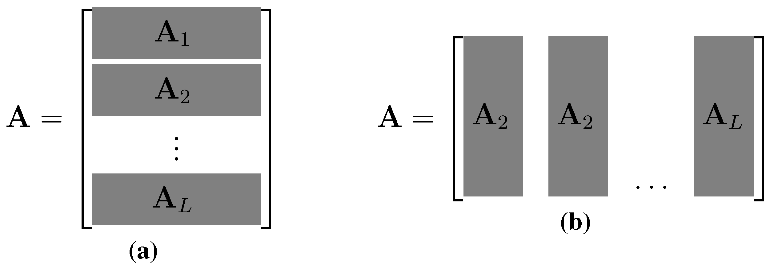
Distributed basis pursuit (DBP) [25] is a recently developed distributed solver based on the aforementioned ADMM. This solver is developed for the noiseless DCS setup and applies to two different signal acquisition models: firstly, the row partitioning, where each node measures a part of y and corresponding rows in A depicted in Figure 3a. Partitioning like this is equivalent to applying the common signal model. A second column partitioning acquisition model is presented in Figure 3b, where each node measures parts of x . This corresponds to a scenario for solving a spatially sparse problem where each sensor measures only a part of the signal. For example, in seismic forward modeling applications [41], where the goal is to find the Green’s function of the model represented by x = x 1 T x 2 T x L T T .
Figure 3. Matrix partitioning for the distributed basis pursuit.
Jsan 03 00001 g003
The main contributions of [25] are, firstly, to derive a generalization to the ADMM; and secondly, for both matrix partitioning scenarios in Figure 3, rewrite the Equation (11) with ϵ = 0 (called basis pursuit (BP)) in suitable forms, such that the generalized ADMM can be applied. The generalization of the ADMM (15) is extended, such that instead of solving for two functions, f and g, it solves the problem for an arbitrary number of functions, f i . The distributed, generalized ADMM solver is then referred to as D-ADMM. Recall that the BP problem is (i.e., the noiseless version of BPDN):
min x ^ 1 subject to A l x ^ = y l l L
By utilizing row partitioning and properties of the network, this problem can now be rewritten in an equivalent form:
min 1 | L | l = 1 c x ^ l 1 + 1 | L | l = 1 + c | L | x ^ l 1
subject to A l x ^ l = y l , l L ,
( B 1 T I N ) x ¯ 1 + ( B 2 T I N ) x ¯ 2 = 0
where B 1 and B 2 are matrices describing the graph, x ¯ 1 and x ¯ 2 are concatenations of x ^ l -vectors, I N is the N × N identity matrix and ⊗ is the Kronecker product. Equation (17) is now exactly of the form for which the generalized ADMM is suited. For this problem, the following analysis result is provided, where k denotes algorithm iteration over networks.
Theorem 2 (Theorem 1 in [25]) 
Assume the given graph is bipartite. Then, for all l, the sequence, { x l ( k ) } , produced by the D-ADMM algorithm converges to a solution of BP.

5.2. D-LASSO

In a paper from Bazerque and Giannakis [42], a distributed LASSO (D-LASSO) (see Equation (12)) solution algorithm is created for spectrum sensing purposes in space, time and frequency. Here, two approaches are introduced: a batch algorithm approach and an online version approach. In the batch algorithm, several nodes co-operate to solve one fixed problem, while in the online version, the task is to track signal changes over time. To shed some insight into this, we provide the outlines of the batched algorithm approach. The D-LASSO problem takes the following form:
min θ 0 , σ l 2 0 l = 1 | L | φ l B l θ σ l 2 1 2 2 + λ 1 T θ
where φ l is some measured vector (cf. y l ), σ l is some parameter associated with non-sparse local noise at the l-th sensor and B l (cf. A l ) is a model of the measurement-system. By iteratively exchanging local estimates θ ^ among the local neighbors and solving a local optimization problem, the following proposition is provided.
Proposition 1 
Provided there always exists a path linking any two nodes of the connected network and with local communications among single-hop neighbors, the estimates, θ ^ , converge to the centralized solution of Equation (18) with some appropriately chosen step-size greater than zero.
For this proposition to hold true, it is assumed that there is local knowledge of the parameter, λ, at each node. In practice, this is not the case, and a separate algorithm is executed in parallel, for the nodes to consent upon an estimate λ = λ max = max l = 1 , , | L | λ l .

6. Greedy Solvers

GP algorithms are ad hoc in nature and endeavor to provide a solution to true Equation (2) by approximation; under certain theoretical conditions, GP algorithms can provide the exact solution. The prime motivation to use GP algorithms is computational simplicity. Using the measurement data in a single-sensor setup, the main principle of the GP algorithms is to detect the underlying support-set of the signal followed by evaluating the associated signal values. Recall that the support-set is a set of indices corresponding to the non-zero elements of a vector. To detect the support-set and find the associated signal values, the GP algorithms use linear algebraic tools, such as matched filter (MF)-based detection and least-squares (LS) estimation. Examples of popular GP algorithms are orthogonal matching pursuit (OMP) [43], subspace pursuit (SP) [44], compressed sampling matching pursuit (CoSaMP) [45], regularized OMP (R-OMP) [46], iterative hard thresholding (IHT) [47], etc., including several others [48,49,50,51].
Before we consider distributed GP solvers, we first discuss the single-sensor algorithms, OMP and SP. These algorithms will then help us to achieve a better understanding for the distributed solvers. In order to more easily explain these algorithms, we introduce the following function:
max _ indices ( a , k ) = { indices corresponding to the k highest amplitude values of a }

6.1. Single-Sensor: Orthogonal Matching Pursuit

Orthogonal matching pursuit (OMP) [52] has a history in statistics tracing back to the 1950s, where it is usually referred to as a stage-wise regression. Tropp et al. [43] performed its theoretical analysis first.
Algorithm 1 Orthogonal matching pursuit (OMP).
Input: y , A , s
Initialization:
k 0
r k y
Iteration:
 1: repeat
 2:   k k + 1
 3:   τ max max _ indices ( A T r k 1 , 1 )
 4:   T k T k 1 τ max
 5:   x ^ T k A T k y
 6:   r k y A T k x ^ T k
 7: until k = s or r k = 0
Output: T ^ T k ; x ^ such that x ^ T k = A T k y  and  x ^ T ¯ k = 0
To detect the support-set, OMP iteratively extends an estimate of the support-set with one index per iteration. By referring to Algorithm 1, we see that OMP uses an MF detection strategy (Step 3) to find the column maximally correlated with r k 1 , which is chosen. The process can equivalently be written:
τ max arg max τ a τ T r k 1
This index, corresponding to the maximally correlated column, is then added to the support-set estimate (Step 4), and a least-squares estimation problem is solved (Step 5) to update the residual vector (Step 6). To achieve the final estimate, OMP uses the least squares estimation on the support-set, T ˜
Regarding performance guarantees for OMP, we note two results in the literature. Davenport and Waking provide in [53] the following theorem.
Theorem 3 (Theorem 3.1 in [53]) 
Suppose that A satisfies the RIP of order s + 1 with isometry constant δ s + 1 < 4 3 s . Then, for any x R N with the number of non-zeros less than or equal to s, OMP will recover x exactly from y = A x in s iterations.
Observe that this theorem 3 only considers the noise-free case ( e = 0 ). Other works have strengthened this result; for example, Liu et al. [54] provides a similar theorem, but with an RIC requirement of δ s + 1 < 1 2 s , or δ s + 1 < 1 1 + s in [55].

6.2. Single Sensor: Subspace Pursuit

The subspace pursuit (SP) algorithm was developed by Dai and Milenkovic [44] and published in 2009. Another algorithm, called CoSaMP [45], closely resembles SP and was developed in the same time. The order of complexity for OMP and SP is comparable, and in our experimental experience, it turns out that they also provide similar performance. We show the SP algorithm in Algorithm 2.
Algorithm 2 Subspace pursuit (SP).
Input: A , s, y
Initialization:
 1: k 0
 2: T k max _ indices A T y , s
 3: r k y A T 0 A T 0 y
Iteration:
 1: repeat
 2:   k k + 1
 3:   T Δ max _ indices A T r k 1 , s
 4:   T ˜ T k 1 T Δ
 5:   x ˜ such that x ˜ T ˜ = A T ˜ y and x ˜ T ˜ c = 0
 6:   T k max _ indices ( x ˜ , s )
 7:   r k y A T k A T k y
 8: until ( r k 2 r k 1 2 )
 9: k k 1                  ( ‘Previous iteration count’ )
Output: T ^ k ; x ^ such that x ^ T k = A T k y and x ^ T k c = 0
The SP algorithm was one of the early GP algorithms to provide convergence and reconstruction bounds similar to those present for convex-relaxation-based reconstruction algorithms.
Theorem 4 (Theorem 9 in [44]) 
Let x R N be such that x 0 s , and let its corresponding measurement be y = A x + e , where e denotes the noise vector. Suppose the sampling matrix satisfies RIC δ 3 s < 0 . 083 . Then, the reconstruction error of the SP algorithm satisfies:
x x ^ 2 C e 2
where C = 1 + δ 3 s + δ 3 s 2 δ 3 s ( 1 δ 3 s ) .
A variation of the theorem, based on a fixed number of iterations as the stopping criteria, was presented by Giryes and Elad:
Theorem 5 (Theorem 2.1 for SP in [3]) 
For an s-sparse vector, x , under the condition that δ 3 s 0 . 139 , after k * = log 2 x 2 A T e T e 2 iterations, where T e = arg max T T T e , the reconstruction accuracy of SP satisfies:
x x ^ 2 C A T k T e 2
where C = 2 7 9 δ 3 s + 7 δ 3 s 2 δ 3 s 3 ( 1 δ 3 s ) 4 21.41 .
Now, we address multi-sensor setups, either in a centralized manner or in a distributed manner.

6.3. S-OMP

The simultaneous-OMP (S-OMP) algorithm, for the DCS problem, was developed by Tropp et al. in [56,57]. This is a centralized algorithm where measurement vectors y l are stacked beside each other to form a measurement matrix, Y . We can then write the centralized problem as:
Y = A X + E
where the signal vector estimates are stacked column-wise in the signal matrix, X . Using the setting of Equation (23), we form the simultaneous sparse approximation (SSA) problem:
min X ^ Y A X ^ F 2 subject to matrix X ^ having at most s nonzero rows
This formulation is equivalent to a problem applying the common signal model, where, additionally to the model, each sensor uses the same measurement matrix, A , that is l , A l = A . We observe that the algorithm should also perform well for the common support-set model, although no such results are available.
The S-OMP algorithm is an extension of the standard OMP algorithm to make it compatible with matrices instead of vectors. Therefore, we can explain the algorithm by describing the differences compared to OMP. In Algorithm 1, Step 3, instead of doing just the standard MF, the absolute sum of the contribution for a given column in A is found. Formally, this can be written as:
τ max arg max τ a τ T R k 1 1
Compare this to the alternative formulation for OMP in Equation (20). The maximal τ max is then added as usual to the support set, and a new residual matrix is derived from:
R k Y A k A k Y
where A T k A T k is one way to form the orthogonal projection matrix.

6.4. SiOMP

The distributed side-information-based OMP (SiOMP) algorithm was developed by Zhang et al. in [58]. SiOMP is built on the assumption of the mixed signal model with the limitation that the algorithm is constructed only for a two-node scenario. Both nodes first execute standard OMP to get first signal estimates, x ^ 1 and x ^ 2 . These estimates are then exchanged, and SiOMP is executed. For node 2, then, the major difference between SiOMP compared to OMP is that the initialization step 2 is replaced with (for k = 0 ):
r k , 2 y 2 A 2 x ^ 1
Similarly, for node 1, we will start with the initialization, r k , 1 y 1 A 1 x ^ 2 . It is clear that the joint components, j , shared by the two users will be removed from the residual and, thus, not again be found by the SiOMP. Based on the cooperation between the two nodes, it is shown that the total number of measurements required for one node is reduced compared to the independent solution.

6.5. DiSP

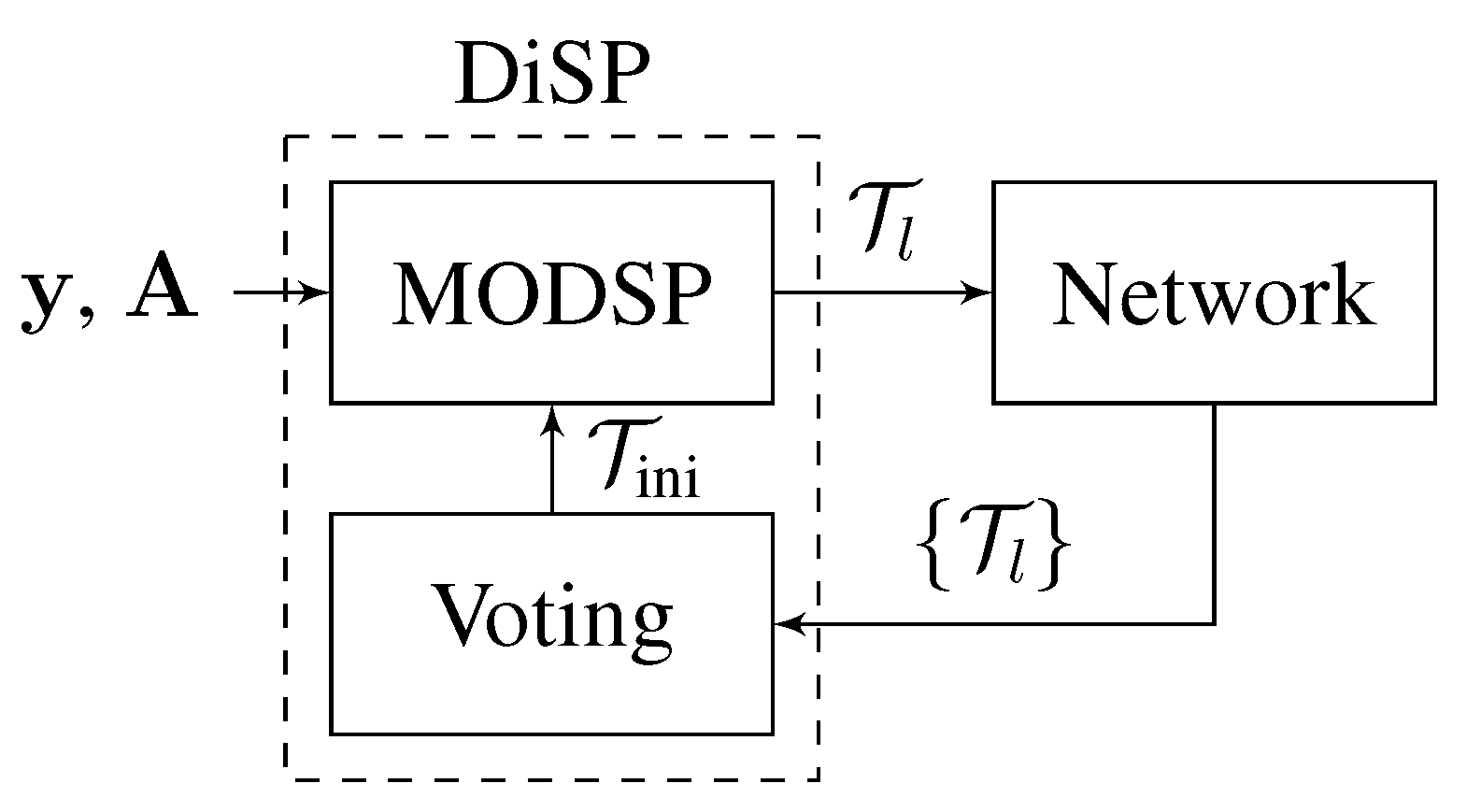
We first developed distributed SP (DiSP) [9,59], which is the first DCS solver based on the mixed support-set model. DiSP solves the DCS problem by exchanging full support-set information. DiSP is constructed assuming the mixed support-set model (see Section 4.5) and is based on a modified SP algorithm (called MODSP) plus a voting procedure, depicted in Figure 4. The modification to SP is such that the algorithm takes an initial support-set as input, meaning it starts searching for the support-set estimate at this initialization point instead of starting in a zero-state. The output of MODSP is, along with the signal estimate, also the support-set estimate, which is broadcast to the node’s neighbors. The initial support is provided by the voting procedure; based on all received support-set estimates, a democratic vote is done, where the support-set indices with the most votes are chosen as the initial support-set. In a theoretical best case, the initial support is found as the joint support, J . DiSP assumes knowledge of the size for the joint support s j = | J | . By iteratively going through the procedure of MODSP, communication, voting, etc., until some convergence, the quality of the signal estimate is experimentally shown to improve.
Figure 4. Algorithm flowchart.
Jsan 03 00001 g004
Proposition 2 (Proposition 2 of [9]) 
For an s-sparse vector, x , under the condition that δ 3 s 0 . 139 , after k * = log 2 x c ini 2 A T e T e 2 iterations, where T c = { 1 , 2 , n } and T e as in Theorem 5, the reconstruction accuracy of MODSP satisfies:
x x ^ 2 C A T e T e 2
where C = 2 7 9 δ 3 s + 7 δ 3 s 2 δ 3 s 3 ( 1 δ 3 s ) 4 21.41 .
By comparing the result in Equation (2) with the one for SP, it is evident that the same worst-case guarantees for DiSP are the same as for SP. This makes sense, since DiSP, when executed in a disconnected network, will perform identically to SP. However, in the average case, DiSP provides for better performance.

6.6. DC-OMP

The distributed and collaborative OMP (DC-OMP) is a recent work by Wimalajeewa et al. [60], developed for support-set detection only. However, after successful support-set detection, it is straight forward to estimate the signal components with LS, as described in the beginning of Section 6.
Based on the underlying assumption of the common signal model, the main idea of the algorithm is to introduce a communication and decision phase in each iteration of the algorithm. Comparing to OMP in Algorithm 1, the communication step is introduced after support index detection (step 3), where each node, l, shares the detected support index, τ max , l , to its outgoing neighbors. Similarly, the node receives support indices from its incoming neighbors. These indices are evaluated in the decision phase, such that every index appearing more than once is selected and added to the support-set estimate. If no index occurs more than one time, only one index is selected, uniformly, at random. It is intuitively clear that, based on the common signal model, indices detected by several sensor nodes are more likely to be correct than those detected by only one. Observe that since the algorithm can add several indices to the support-set in each iteration, it requires less iterations than OMP.

6.7. DPrSP

We also developed distributed predictive SP (DPrSP) in [31] based on DiSP and the predictive SP algorithm of [61,62]. The DPrSP algorithm is designed to exploit correlations among the joint support-set components, as described by the signal model of common support-set model with correlations (see Section 4.6). In the core of this algorithm is the PrSP algorithm, which is a statistical modification of the SP algorithm. The overall block diagram of DPrSP will be similar to the Figure 4, where MODSP is replaced with PrSP algorithm and voting is replaced with a linear minimum mean square error (LMMSE) estimator. The LMMSE estimate considers second order statistical parameters of signals and noise.

6.8. D-IHT

Patterson et al. presents a distributed solver called D-IHT in [63]. This algorithm is developed based on the common signal model. Using multiple computational nodes, the algorithm exactly implements a greedy pursuit algorithm, called iterative hard thresholding (IHT). Now, we briefly explain the IHT algorithm. The IHT can be neatly written in one iteration as follows:
x ^ k H s x ^ k 1 + μ A T ( y A x ^ k 1 )
where H s is a non-linear operator that sets all but the s largest-in-magnitude elements to zero, and μ is a suitable step size. If μ < 2 λ max ( A T A ) , where λ max is the largest eigenvalue of A T A , then IHT converges [47]. Observe the structural similarity to OMP: y A x ^ k 1 resembles the residual (Step 3), A T resembles the matched filter (Step 3) and H s resembles the operation of picking the largest component.
D-IHT executes Equation (29) exactly using multiple computational nodes. In D-IHT, either one node acts as a leader node and has full contact to all other nodes or the network is fully connected (then every node can do the job of the leader node). For iteration k, each node, l, locally solves the following local computation:
z l , k μ A l T ( y l A l x k )
All nodes then send their result to the leader node, which then has { z l , k } l L . The leader solves the global computation problem, which is:
x k + 1 H s x k + l = 1 | L | z l , k
and distributes x k + 1 back to all the nodes for further iterations. In a sense, this algorithm is a centralized solver, but the central node only does limited computation.

6.9. Overview of Distributed Greedy Pursuits

We now provide a summary of the algorithms briefly presented, listing if they are a distributed algorithm and to which signal models they may be applied. We present the result in Table 1.
Table 1. Applicability of distributed algorithms. S-OMP, simultaneous orthogonal matching pursuit; SiOMP, side-information-based OMP; DC-OMP, distributed and collaborative OMP; DiSP, distributed subspace pursuit; DPrSP, distributed predictive SP; D-IHT, distributed iterative hard thresholding; D-BPDN, distributed basis pursuit denoising; D-LASSO, distributed least absolute shrinkage and selection operator.
Jsan 03 00001 i001

7. Simulations

For several algorithms, analytical reconstruction guarantees are available in the literature. These guarantees are expressed in terms of bounds on the performance and, in general, provide certain requirements of the sensing matrix. The requirements are practically difficult to fulfill, and the bounds are the loose, worst-case, bounds. Therefore, computer simulation is a powerful tool to provide insight into how we can expect an algorithm to perform in practice.

7.1. Performance Measures

Two performance measures that are often used in the literature are average signal cardinality error (ASCE) and signal-to-reconstruction-error ratio (SRER). ASCE is defined as:
ASCE = 1 E | T T ^ | | T | ,
where T T is the true support-set and T ^ is the estimated support. The ASCE is used in [9,49,64] for performance evaluation. Note that we want to minimize the ASCE. Then, the second performance measure, SRER, is defined as:
SRER = E { x 2 2 } E { x x ^ 2 2 } .
For good reconstruction, SRER is expected to be as high as possible.

7.2. Experiments

For the purpose of simulations, we introduce the fraction of measurement α as:
α = m n .
It would be interesting to provide simulation comparison between all algorithms described in this paper. However, we, the authors, only have access to DPrSP and DiSP codes; the codes are also available online (https://sites.google.com/site/saikatchatt/).
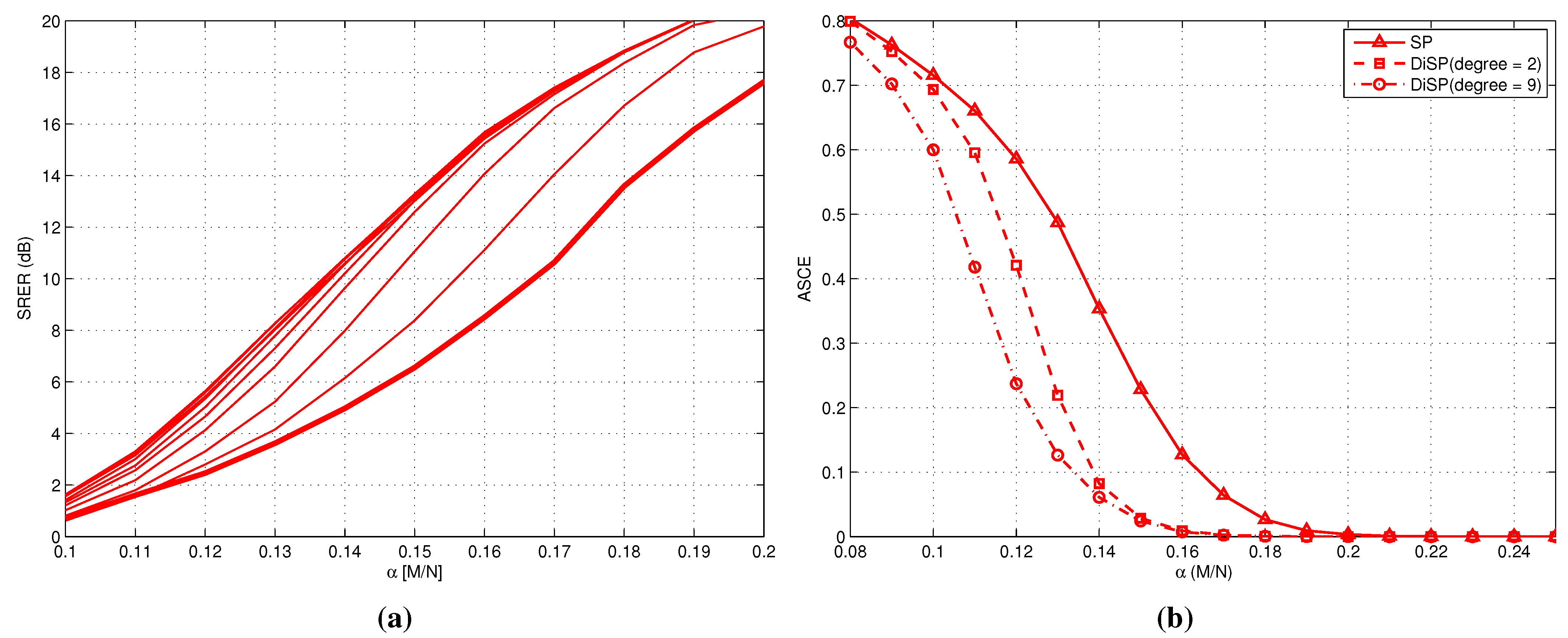
In Figure 5, we demonstrate in two figures the performance of DiSP in a network with ten users. In both figures, each data-point is averaged over 100 measurement-matrices and 100 signal-vectors (i.e., an average of 10 4 simulations) to provide smooth performance curves. In Figure 5a, we demonstrate how the performance of DiSP improves systematically as the network connectivity is increased (using the structured forward circular network model). In this figure, the signal-to-measurement-noise ratio (SMNR = E ( x 2 2 ) E ( e 2 2 ) ) is 20 dB. The signal model is the mixed support-set model with s j , l = s j = 10 , s i , l = s i = 10 and signal dimensions of n = 500 for all users. The curve in the bottom represents the standard, disconnected, SP algorithm. Then, the second curve, above SP, is the performance of DiSP using the forward circular network model of degree one. Increasing the degrees from one up until degree nine, we see the performance of all intermediate networks for this particular algorithm. Note that degree nine is the highest possible degree in this setup and corresponds to a fully connected network. In Figure 5b, we show the performance of DiSP using the ASCE in a setup with a noise-free environment. The zero ASCE corresponds to exact reconstruction in the noise-free case. We see that the α threshold for exact reconstruction is better in DiSP than the standard SP.
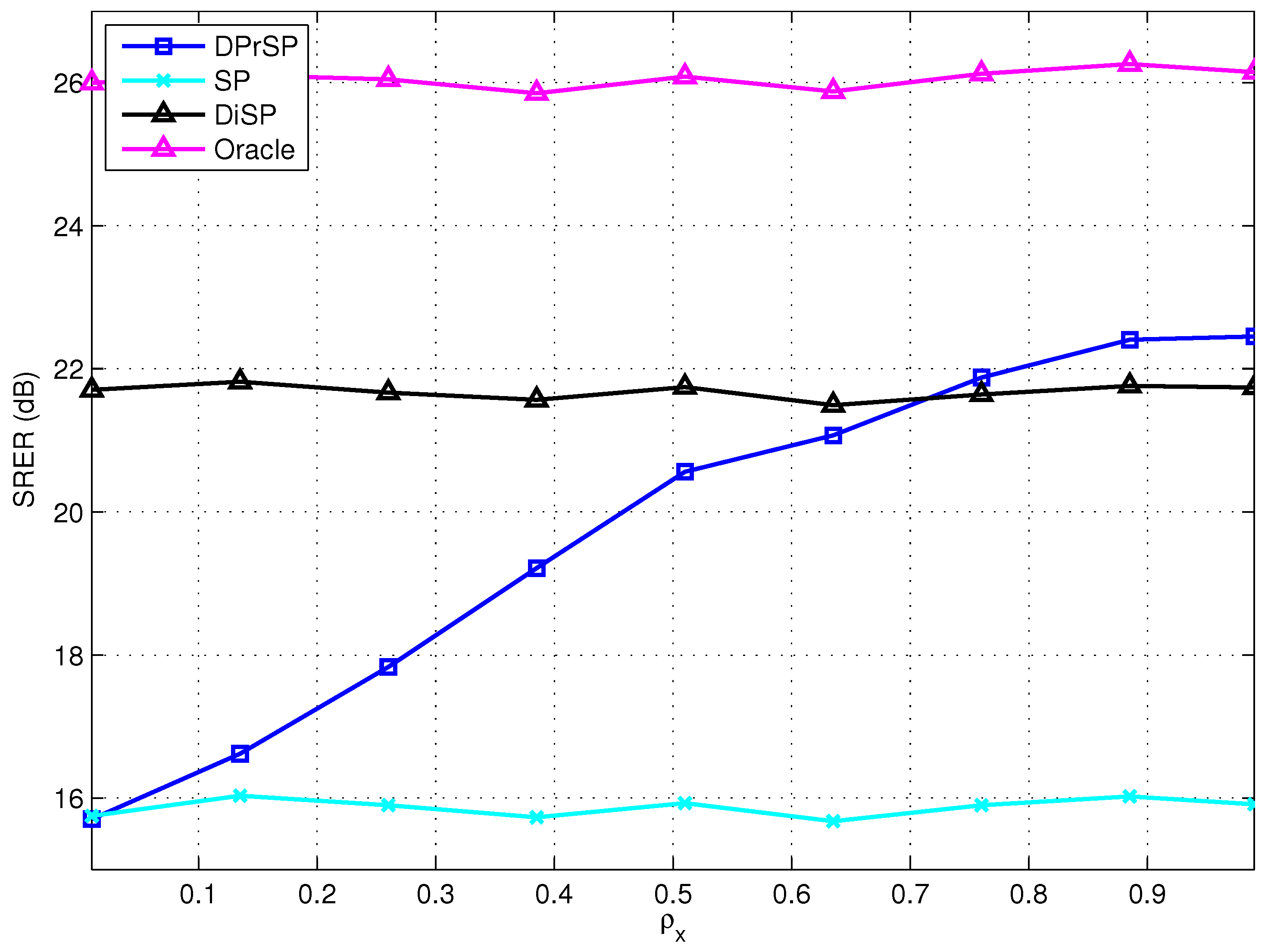
In Figure 6, we show the performance for DPrSP in a plot with SRER along the x-axis and ρ x along the y-axis; ρ x is the correlation parameter for the mixed support-set model with correlations described in Section 4.6. Here, we have ten sensor nodes and use the forward circular network model with degree two. Each data-point is an average over 10 4 simulations, and we compare between SP, DiSP and an oracle estimator. The oracle performance is the least-squares solution given the knowledge of the true support-set of the signal. We see that as ρ x increases, the performance of DPrSP increases, too. We also notice that DiSP performs well, and it is not until ρ x = 0 . 7 that DPrSP actually outperforms DiSP.
Figure 5. Performance of DiSP using the forward circular network model with 10 users. In (a), we show α vs. signal-to-reconstruction-error ratio (SRER) curve of DiSP using network degree of one through nine, where degree 9 is a fully connected network. The bottom fat line corresponds to standard SP and the topmost line a fully connected network. In (b), we show α vs. average signal cardinality error (ASCE) curve of DiSP using network degree of two and nine, where nine is a fully connected network.
Jsan 03 00001 g005
Figure 6. SRER vs. ρ x curve for DiSP and DPrSP.
Jsan 03 00001 g006

8. Discussion and Open Problems

In a network of sensor nodes that can cooperate, theoretical insights are available under certain restrictions; for example, for convex solvers in a DCS setup, measurement requirements are available when all sensors measures the same signal (i.e., the common signal model); for GP solvers in a DCS setup, theoretical insights are available for centralized solvers using the common signal model. However, for a DCS problem with more interesting signal models (i.e., common support-set model, mixed support-set model, etc.), such theoretical insights are not available; through simulations, we show that significant performance gains can be achieved for such scenarios. For practical implementation, we notice that the communication overhead in terms of time and cost is an aspect not much discussed in the DCS literature. We expect that in order to make the DCS problems attractive in the future, the challenge of deriving strong theoretical insights remains a major open problem.

Conflicts of Interest

The authors declare no conflict of interest.

References

  1. Donoho, D.L. Compressed sensing. IEEE Trans. Inf. Theory 2006, 52, 1289–1306. [Google Scholar] [CrossRef]
  2. Candés, E.J.; Tao, T. Near-optimal signal recovery from random projections: Universal encoding strategies? IEEE Trans. Inf. Theory 2006, 52, 5406–5425. [Google Scholar] [CrossRef]
  3. Giryes, R.; Elad, M. RIP-based near-oracle performance guarantees for SP, CoSaMP, and IT. IEEE Trans. Signal Process. 2012, 60, 1465–1468. [Google Scholar] [CrossRef]
  4. Candés, E.J.; Tao, T. Decoding by linear programming. IEEE Trans. Inf. Theory 2005, 51, 4203–4215. [Google Scholar] [CrossRef]
  5. Donoho, D.L.; Huo, X. Uncertainty principles and ideal atomic decomposition. IEEE Trans. Inf. Theory 2001, 47, 2845–2862. [Google Scholar] [CrossRef]
  6. Cohen, A.; Dahmen, W.; Devore, R. Compressed sensing and best k-term approximation. J. Amr. Math. Soc. 2009, 211–231. [Google Scholar]
  7. Feuer, A.; Nemirovski, A. On sparse representation in pairs of bases. IEEE Trans. Inf. Theory 2003, 49, 1579–1581. [Google Scholar] [CrossRef]
  8. Raskutti, G.; Wainwright, M.; Martin, J.; Yu, B. Restricted eigenvalue properties for correlated gaussian designs. J. Mach. Learn. Res. 2010, 11, 2241–2259. [Google Scholar]
  9. Sundman, D.; Chatterjee, S.; Skoglund, M. Distributed Greedy Pursuit Algorithms. Available online: http://arxiv.org/abs/0901.3403 (accessed on 10 December 2013).
  10. Erdős, P.; Rényi, A. On random graphs. Publ. Math. 1959, 6, 290–297. [Google Scholar]
  11. Watts, D.; Strogatz, S. Collective dynamics of “small-world” networks. Nature 1998, 393, 409–410. [Google Scholar] [CrossRef] [PubMed]
  12. Penrose, M. Random Geometric Graphs. In Random Geometric Graphs; Oxford University Press: Oxford, UK, 2004. [Google Scholar]
  13. Barabási, A.; Albert, R. Emergence of scaling in random networks. Science 1999, 286, 509–512. [Google Scholar] [PubMed]
  14. Elias, P.; Feinstein, A.; Shannon, C.E. A note on the maximum flow through a network. IRE Trans. Inf. Theory 1956, 4, 117–119. [Google Scholar] [CrossRef]
  15. Ford, L.R.; Fulkerson, D.R. Maximal flow through a network. Can. J. Math. 1956, 8, 399–404. [Google Scholar] [CrossRef]
  16. Blasco-Serrano, R.; Zachariah, D.; Sundman, D.; Thobaben, R.; Skoglund, M. An Achievable Measurement Rate-MSE Tradeoff in Compressive Sensing through Partial Support Recovery. In Proceedings of IEEE International Conference on Acoustics, Speech and Signal Processing (ICASSP 2013), Vancouver, BC, Canada, 26–31 May 2013; pp. 6426–6430.
  17. Feizi, S.; Medard, M. A Power Efficient Sensing/Communication Scheme: Joint Source-Channel-Network Coding by Using Compressive Sensing. In Proceedings of AnnualAllerton Conference on Communication, Control, and Computing (Allerton 2011), Champaign, IL, USA, 2–4 October 2013; pp. 1048–1054.
  18. Feizi, S.; Medard, M.; Effros, M. Compressive Sensing over Networks. In Proceedings of IEEE Annual Allerton Conference on Communication, Control, and Computing (Allerton 2010), Monticello, IL, USA, 29 September–1 October; pp. 1129–1136.
  19. Goyal, V.K.; Fletcher, A.K.; Rangan, S. Compressive sampling and lossy compression. IEEE Signal Process. Mag. 2008, 25, 48–56. [Google Scholar] [CrossRef]
  20. Sun, J.Z.; Goyal, V.K. Optimal Quantization of Random Measurements in Compressed Sensing. In Proceedings of 2009 IEEE International Symposium on Information Theory, Seoul, Korea, 28 June–3 July 2009; pp. 6–10.
  21. Shirazinia, A.; Chatterjee, S.; Skoglund, M. Analysis-by-synthesis quantization for compressed sensing measurements. IEEE Trans. Signal Process. 2013, 61, 5789–5800. [Google Scholar] [CrossRef]
  22. Ming, Y.; Yi, Y.; Osher, S. Robust 1-bit compressive sensing using adaptive outlier pursuit. IEEE Trans. Signal Process. 2012, 60, 3868–3875. [Google Scholar] [CrossRef]
  23. Wei, D.; Milenkovic, O. Information theoretical and algorithmic approaches to quantized compressive sensing. IEEE Trans. Commun. 2011, 59, 1857–1866. [Google Scholar]
  24. Zymnis, A.; Boyd, S.; Candés, E. Compressed sensing with quantized measurements. IEEE Signal Process. Lett. 2010, 17, 149–152. [Google Scholar] [CrossRef]
  25. Mota, J.F.C.; Xavier, J.M.F.; Aguiar, P.M.Q.; Püschel, M. Distributed basis pursuit. IEEE Trans. Signal Process. 2012, 60, 1942–1956. [Google Scholar] [CrossRef]
  26. Baron, D.; Duarte, M.F.; Wakin, M.B.; Sarvotham, S.; Baraniuk, R.G. Distributed Compressive Sensing. Available online: http://arxiv.org/abs/0901.3403 (accessed on 10 December 2013).
  27. Park, J.; Hwang, S.; Yang, J.; Kim, D.K. Generalized Distributed Compressive Sensing. Available online: http://arxiv.org/abs/1211.6522 (accessed on 10 December 2013).
  28. Sundman, D.; Chatterjee, S.; Skoglund, M. On the Use of Compressive Sampling for Wide-Band Spectrum Sensing. In Proceedings of IEEE International Symposium on Signal Processing and Information Technology (ISSPIT 2010), Luxor, Egypt, 15–18 December 2010; pp. 354–359.
  29. Kirmani, A.; Colaco, A.; Wong, F.N.C.; Goyal, V.K. CoDAC: A Compressive Depth Acquisition Camera Rramework. In Proceedings of IEEE International Conference on Acoustics, Speech and Signal Processing (ICASSP 2012), Kyoto, Japan, 25–30 March 2012; pp. 5425–5428.
  30. Wu, P.K.T.; Epain, N.; Jin, C. A Dereverberation Algorithm for Spherical Microphone Arrays Using Compressed Sensing Techniques. In Proceedings of IEEE International Conference on Acoustics, Speech and Signal Processing (ICASSP 2012), Kyoto, Japan, 25–30 March 2012; pp. 4053–4056.
  31. Sundman, D.; Zachariah, D.; Chatterjee, S.; Skoglund, M. Distributed Predictive Subspace Pursuit. In Proceedings of International Conference on Acoustics, Speech, and Signal Processing, Vancouver, BC, Canada, 26–31 May 2013.
  32. Candés, E. The restricted isometry property and its implications for compressed sensing. Rendus Math. 2008, 346, 589–592. [Google Scholar] [CrossRef]
  33. Candés, E.J.; Wakin, M.B. An introduction to compressive sampling. IEEE Signal Process. Mag. 2008, 25, 21–30. [Google Scholar] [CrossRef]
  34. Davenport, M.A.; Boufounos, P.T.; Wakin, M.B.; Baraniuk, R.G. Signal processing with compressive measurements. IEEE J. Sel. Topics Signal Process. 2010, 4, 445–460. [Google Scholar] [CrossRef]
  35. Boyd, S.; Parikh, E.; Chu, E.; Peleato, B.; Eckstein, J. Distributed optimization and statistical learning via the alternating method of multipliers. Found. Trends Mach. Learn. 2011, 3, 1–122. [Google Scholar] [CrossRef]
  36. Dantzig, G.B. Linear Programming and Extensions; Princeton University Press: Princeton, NJ, USA, 1963. [Google Scholar]
  37. Dutta, H.; Kargupta, H. Distributed Linear Programming and Resource Management for Data Mining in Distributed Environments. In Proceedings of IEEE International Conference on Data Mining Workshops (ICDMW 2008), Pita, Italy, 15–19 December 2008; pp. 543–552.
  38. Yarmish, G. A Distributed Implementation of the Simplex Method. Ph.D. Thesis, Polytechnic University, HongKong, China, 2001. [Google Scholar]
  39. Hall, J.A.J.; McKinnon, K.I.M. Update Procedures for the Parallel Revised Simplex Method; Technical Report; University of Edingburgh: Edinburgh, UK, 1992. [Google Scholar]
  40. Craig, S.; Reed, D. Hypercube Implementation of the Simplex Algorithm. In Proceedings of the Third Conference on Hypercube Concurrent Computers and Applications, Pasadena, CA, USA, 19–20 January 1988; pp. 1473–1482.
  41. Neelamani, R.; Krohn, C.E.; Krebs, J.R.; Deffenbaugh, M.; Anderson, J.E.; Romberg, J.K. Efficient Seismic Forward Modeling Using Simultaneous Random Sources and Sparsity. In Proceedings of SEG International Exposition and 78th Annual Meeting, Las Vegas, NV, USA, 9–14 November 2008.
  42. Bazerque, J.A.; Giannakis, G.B. Distributed spectrum sensing for cognitive radio networks by exploiting sparsity. IEEE Trans. Signal Process. 2010, 58, 1847–1862. [Google Scholar] [CrossRef]
  43. Tropp, J.A.; Gilbert, A.C. Signal recovery from random measurements via orthogonal matching pursuit. IEEE Trans. Inf. Theory 2007, 53, 4655–4666. [Google Scholar] [CrossRef]
  44. Dai, W.; Milenkovic, O. Subspace pursuit for compressive sensing signal reconstruction. IEEE Trans. Inf. Theory 2009, 55, 2230–2249. [Google Scholar] [CrossRef]
  45. Needell, D.; Tropp, J.A. CoSaMP: Iterative signal recovery from incomplete and inaccurate samples. Appl. Comput. Harmon. Anal. 2009, 26, 301–321. [Google Scholar] [CrossRef]
  46. Needell, D.; Vershynin, R. Signal recovery from incomplete and inaccurate measurements via regularized orthogonal matching pursuit. IEEE J. Sel. Topics Signal Process. 2010, 4, 310–316. [Google Scholar] [CrossRef]
  47. Blumensath, T.; Davies, M.E. Iterative hard thresholding for compressed sensing. Appl. Comput. Harmon. Anal. 2009, 27, 265–274. [Google Scholar] [CrossRef]
  48. Chatterjee, S.; Sundman, D.; Vehkapera, M.; Skoglund, M. Projection-based and look-ahead strategies for atom selection. IEEE Trans. Signal Process. 2012, 60, 634–647. [Google Scholar] [CrossRef]
  49. Sundman, D.; Chatterjee, S.; Skoglund, M. Look Ahead Parallel Pursuit. In Proceedings of IEEE Swedish Communication Technologies Workshop (Swe-CTW 2011), Stockholm, Sweden, 19–21 October 2011; pp. 114–117.
  50. Sundman, D.; Chatterjee, S.; Skoglund, M. FROGS: A Serial Reversible Greedy Search Algorithm. In Proceedings of IEEE Swedish Communication Technologies Workshop (Swe-CTW 2012), Lund, Sweden, 24–26 October 2012.
  51. Sundin, M.; Sundman, D.; Jansson, M. Beamformers for Sparse Recovery. In Proceedings of IEEE International Conference on Acoustics, Speech and Signal Processing (ICASSP 2013), Vancouver, BC, Canada, 26–31 May 2013; pp. 5920–5924.
  52. Pati, Y.C.; Rezaiifar, R.; Krishnaprasad, P.S. Orthogonal Matching Pursuit: Recursive Function Approximation with Applications to Wavelet Decomposition. In Proceedings of the 27th Annual Asilomar Conference on Signals, Systems, and Computers, Pacific Grove, CA, USA, 3–6 November 2013; pp. 40–44.
  53. Davenport, M.A.; Wakin, M.B. Analysis of orthogonal matching pursuit using the restricted isometry property. IEEE Trans. Inf. Theory 1993, 56, 4395–4401. [Google Scholar] [CrossRef]
  54. Liu, E.; Temlyakov, V.N. The orthogonal super greedy algorithm and applications in compressed sensing. IEEE Trans. Inf. Theory 2012, 58, 2040–2047. [Google Scholar] [CrossRef]
  55. Maleh, R. Improved RIP Analysis of Orthogonal Matching Pursuit. Available online: http://arxiv.org/abs/1102.4311 (accessed on 10 December 2013).
  56. Tropp, J.A.; Gilbert, A.C.; Strauss, M.J. Simultaneous Sparse Approximation via Greedy Pursuit. In Proceedings of IEEE International Conference on Acoustics, Speech, and Signal Processing, Honolulu, HI, USA, 18–23 March 2005; pp. 721–724.
  57. Tropp, J.A.; Gilbert, A.C.; Strauss, M.J. Algorithms for simultaneous sparse approximation. Part I: Greedy pursuit. Signal Process. 2006, 86, 572–588. [Google Scholar] [CrossRef]
  58. Zhang, W.; Ma, C.; Wang, W.; Liu, Y.; Zhang, L. Side Information Based Orthogonal Matching Pursuit in Distributed Compressed Sensing. In Proceedings of IEEE International Conference on Network Infrastructure and Digital Content (ICNIDC 2010), Beijing, China, 24–26 September 2010; pp. 80–84.
  59. Sundman, D.; Chatterjee, S.; Skoglund, M. A Greedy Pursuit Algorithm for Distributed Compressed Sensing. In Proceedings of IEEE International Conference on Acoustics, Speech and Signal Processing (ICASSP 2012), Kyoto, Japan, 25–30 March 2012; pp. 2729–2732.
  60. Wimalajeewa, T.; Varshney, P.K. Cooperative Sparsity Pattern Recovery in Distributed Networks via Distributed-OMP. In Proceedings of IEEE International Conference on Acoustics, Speech, and Signal Processing (ICASSP 2013), Vancouver, BC, Canada, 26–31 May 2013.
  61. Zachariah, D.; Chatterjee, S.; Jansson, M. Dynamic Subspace Pursuit. In Proceedings of IEEE International Conference on Acoustics, Speech and Signal Processing (ICASSP 2012), Kyoto, Japan, 25–30 March 2012; pp. 3605–3608.
  62. Zachariah, D.; Chatterjee, S.; Jansson, M. Dynamic iterative pursuit. IEEE Trans. Signal Process. 2012, 60, 4967–4972. [Google Scholar] [CrossRef]
  63. Patterson, S.; Eldar, Y.C.; Keidar, I. Distributed Sparse Signal Recovery for Sensor Networks. In Proceedings of IEEE International Conference on Acoustics, Speech, and Signal Processing (ICASSP 2013), Vancouver, BC, Canada, 26–31 May 2013.
  64. Reeves, G.; Gastpar, M. A Note on Optimal Support Recovery in Compressed Sensing. In Proceedings of the Annual Asilomar Conference on Signals, Systems, and Computers, Pacific Grove, CA, USA, 4–7 November 2009; pp. 1576–1580.