An Adaptive Strategy for an Optimized Collision-Free Slot Assignment in Multichannel Wireless Sensor Networks

Abstract
:1. Introduction
- Retransmission of a message that has not been acknowledged at the MAC layer.
- Temporary change in the application needs due to alarms, for instance. Alarms are associated with strong delay requirements and must be reliably delivered to the sink. Several possibilities exist:
- –
- if a slot was assigned to the sender node, the alarm is sent first, taking the place of the regular data. This regular data will then be sent in an additional slot, granted by the adaptive solution.
- –
- if no slot was assigned to the sender node; in the worst case, the alarm is sent in the next cycle following the control message requesting the alarm transfer.
2. Related Work
2.1. Multichannel Slot Assignment
2.2. Adaptive Slot Assignment
- A slot spreading algorithm: Nodes in TDMA-ASAP steal only from adjacent or nearby slots. The proposed algorithm spreads out children slots evenly in the schedule.
- Stealing both in upstream and downstream communication: The authors assume that any cycle consists of upstream slots and optional downstream slots spread throughout the cycle. Since downstream slots are not necessary in every cycle, they can be stolen by upstream communications. If the children do not receive a control message from their parents, they treat the downstream slot reserved for their parent as a stealable slot.
3. Multichannel Slot Assignment with Heterogeneous Demands
3.1. Multichannel Slot Assignment Problem
3.2. Assumptions
- The primary assumptions that are required by the solutions proposed (scheduling algorithms), the computation of the theoretical bounds and the performance evaluation of the solution;
- The secondary assumptions that are not required by the solutions to work correctly. They are only introduced to simplify the computation of the theoretical bounds and the performance evaluation.
3.2.1. Primary Assumptions
3.2.2. Secondary Assumptions
3.3. Theoretical Bounds on the Number of Slots for a Raw Data Convergecast
3.3.1. Linear Networks
- In the current time slot, ,
- –
- if t is odd, any node that is hops away from the sink, with , where N is the number of nodes;
- –
- if t is even, any node that is hops away from the sink, with .
- the child of the sink in the next contiguous slots.
- In the first slot, the sink child transmits one packet of its own data.
- In any odd slot, t, with , the sink child transmits any packet received from its children in the previous slot. Consequently this schedule ensures that any node, different from the sink and its child, transmits simultaneously with its grand-parent. Since these two nodes are conflicting on the same channel, they are only allowed to transmit on different channels. For instance, if we consider the odd slots, nodes at depth will transmit on the first available channel, whereas nodes at depth will transmit on the second available channel. For the even slots, nodes at depth will transmit on the first available channels, and nodes at depth will transmit on the second available channel.
- In the slot, the sink child transmits the last last packet received from its child.
- In the next slots, it transmits its own packets.
3.3.2. Multi-Line Networks
3.3.3. Tree Networks
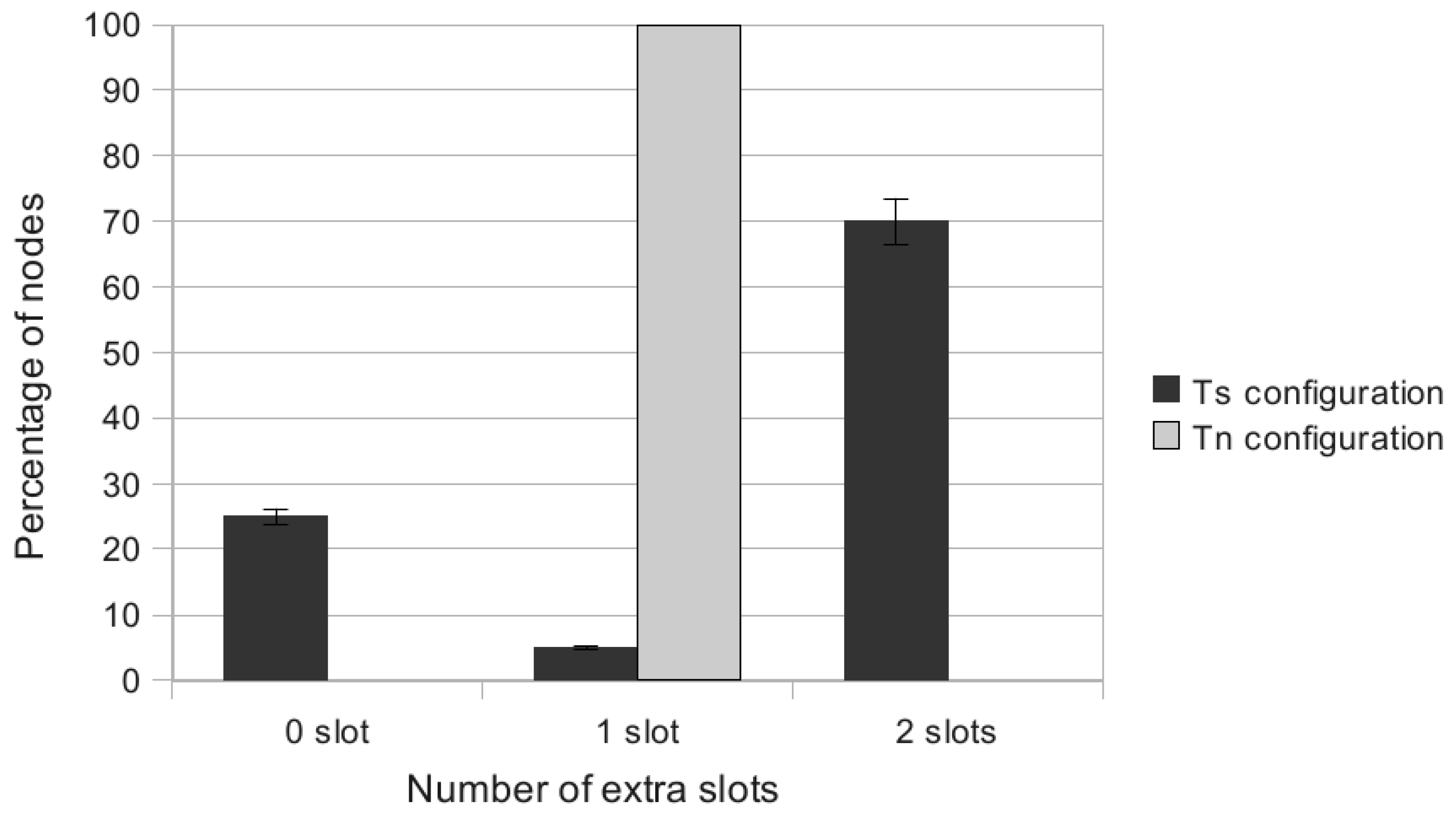
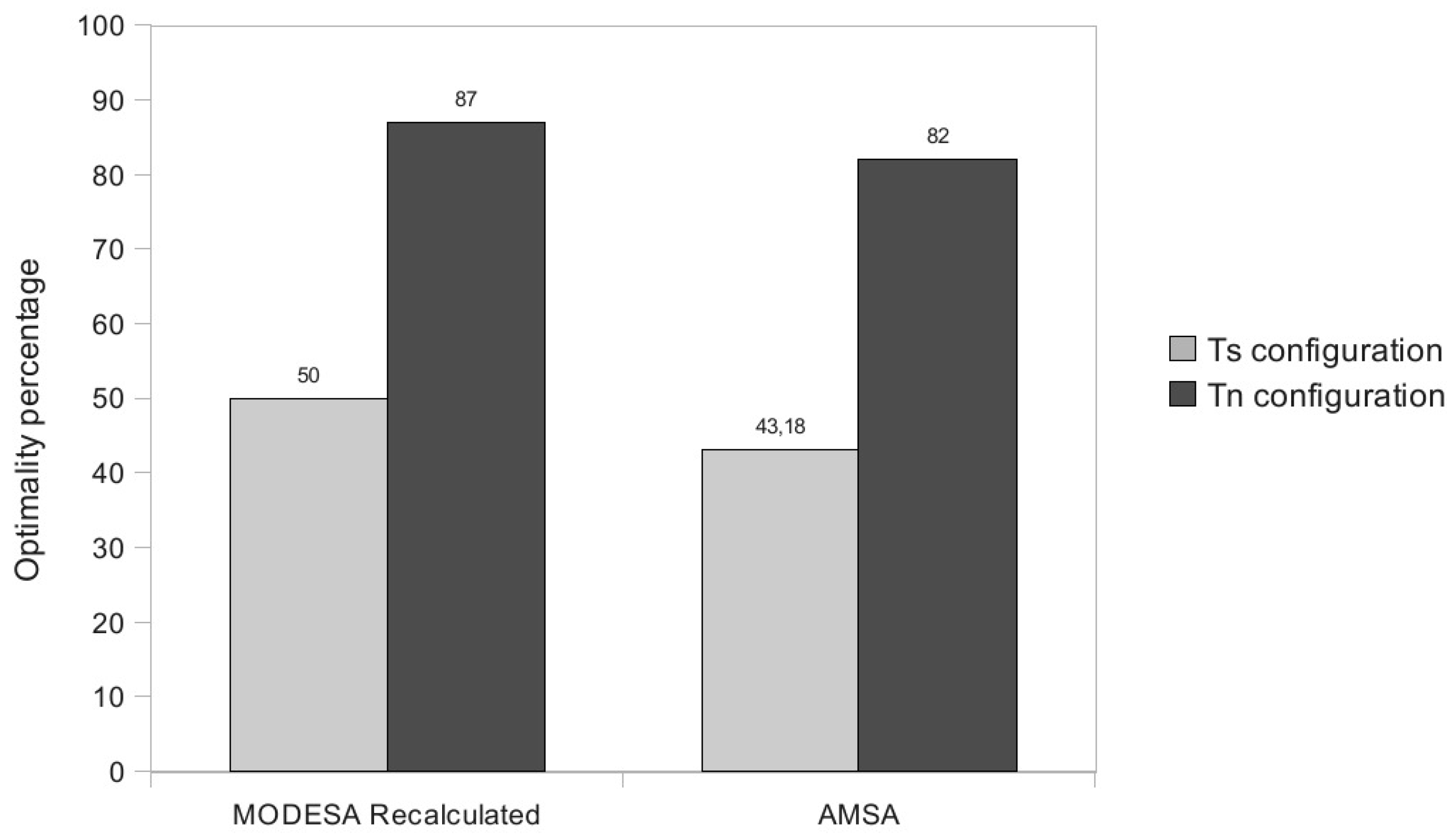
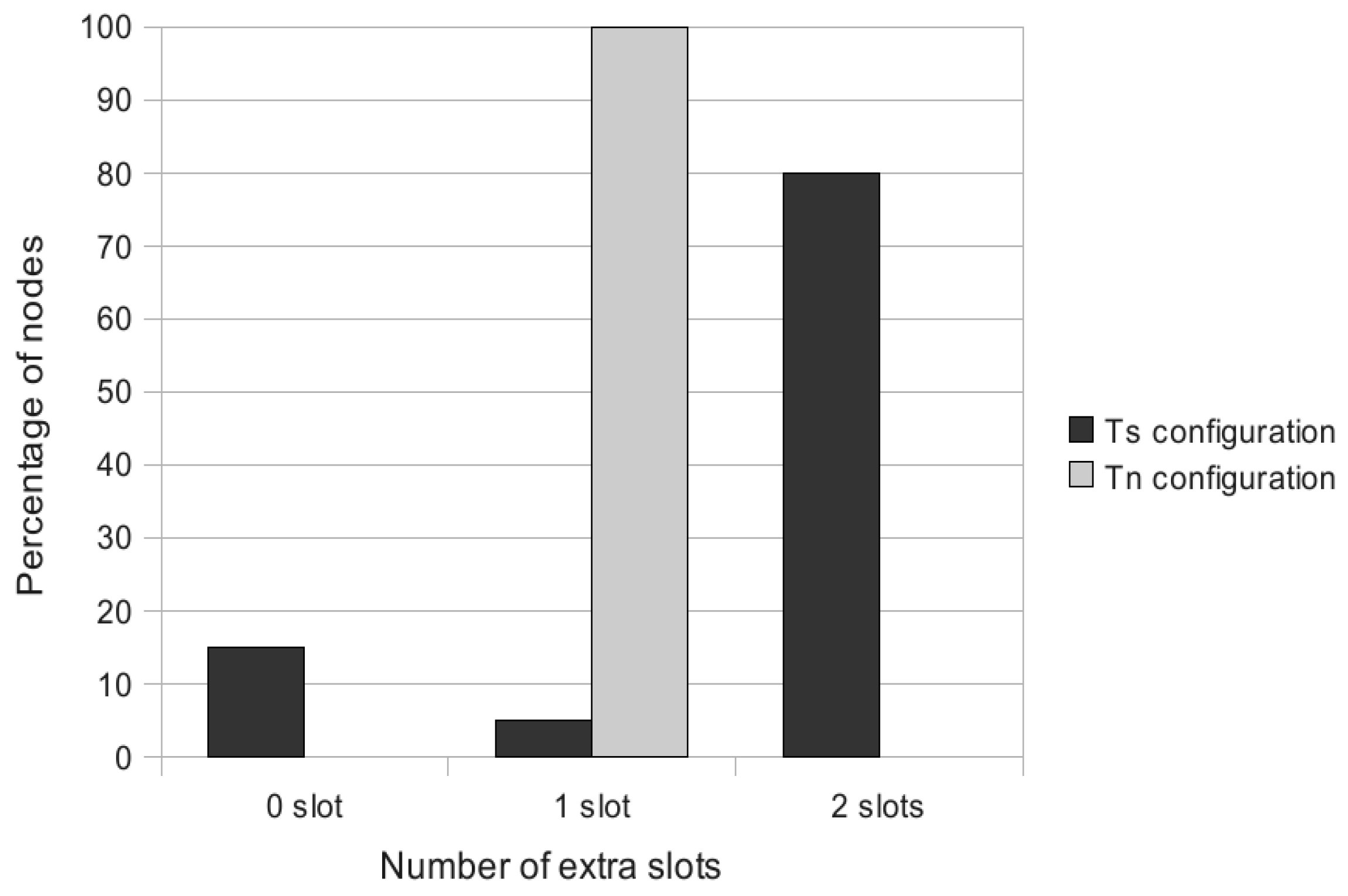
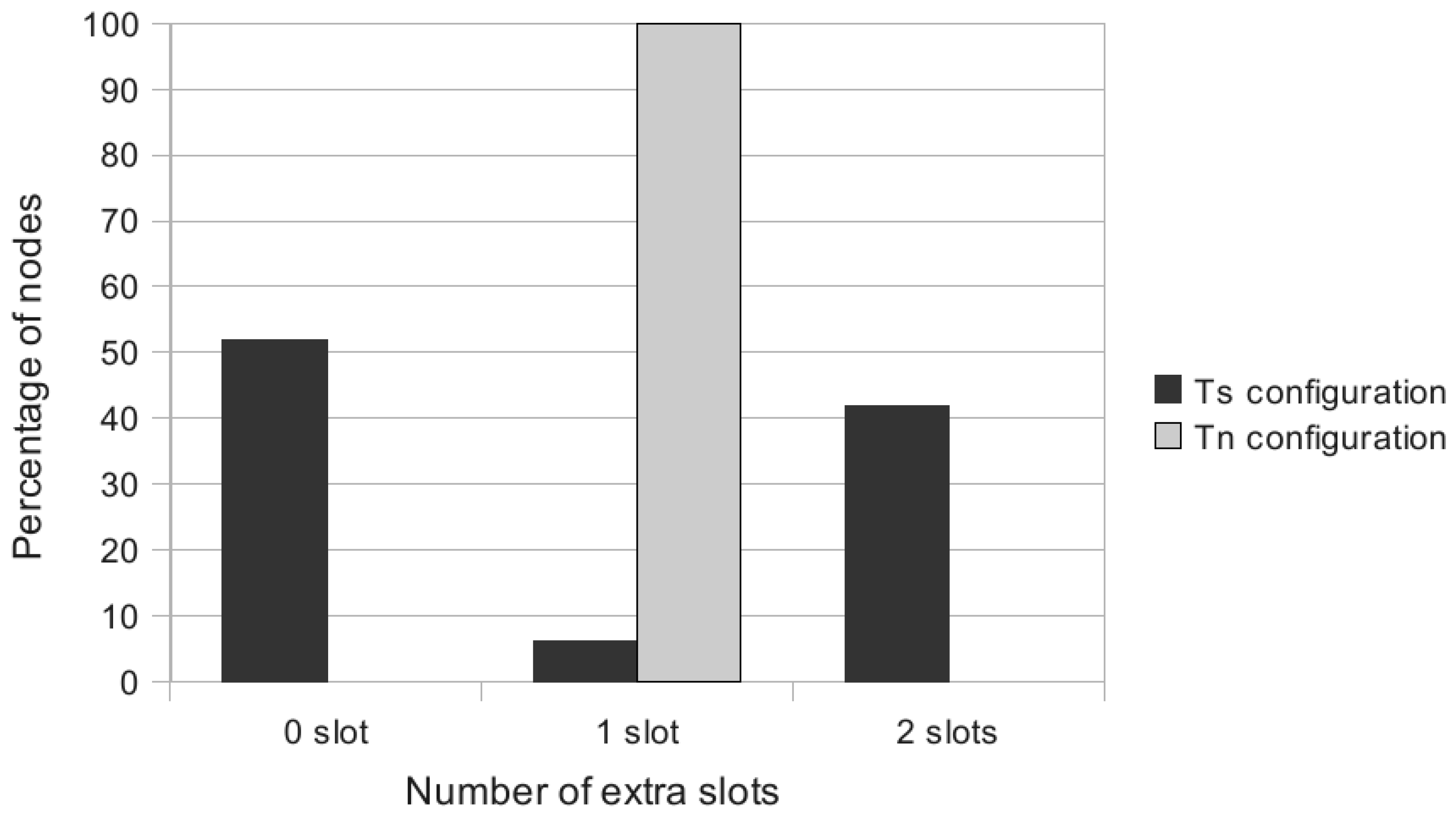
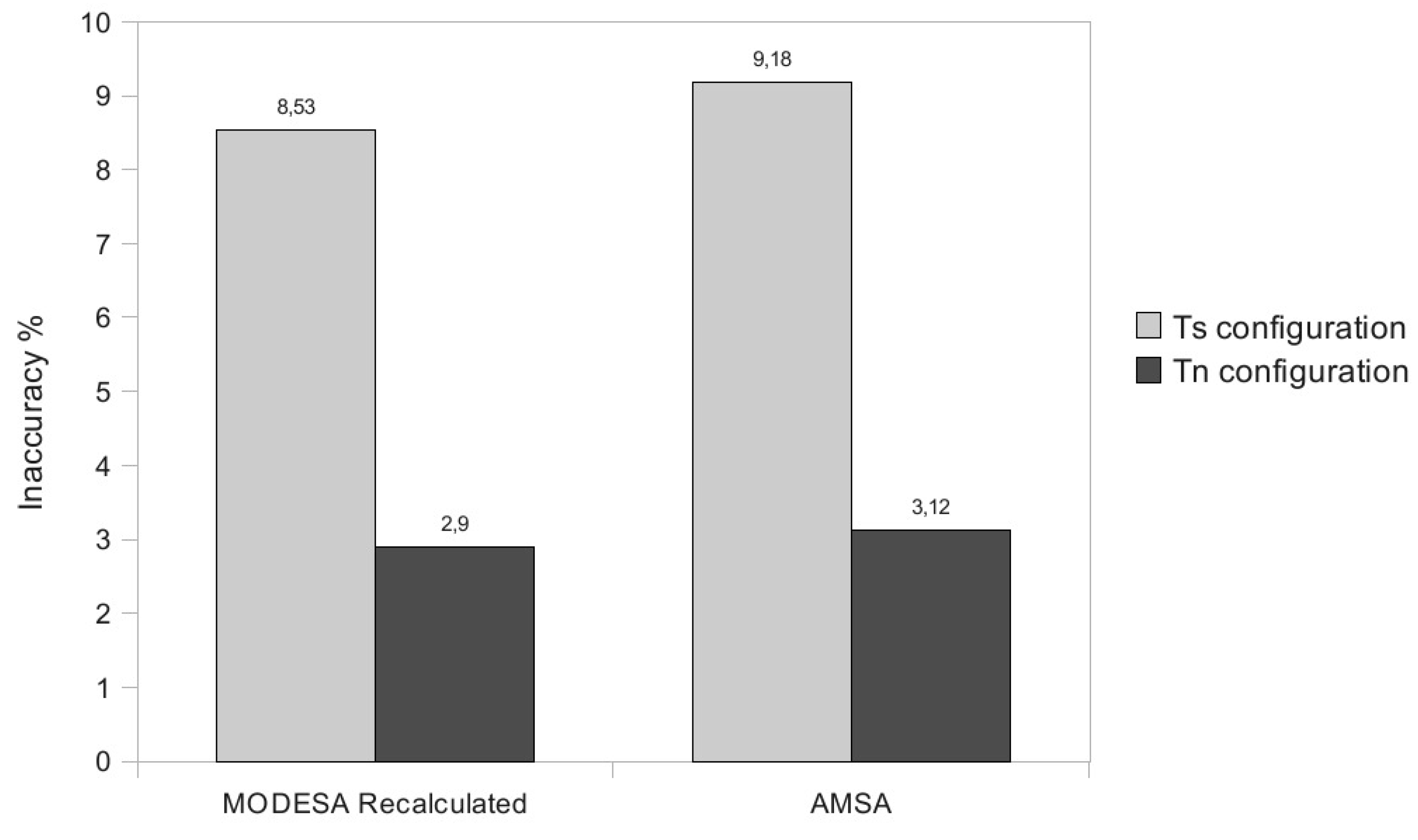
3.3.4. and Configurations
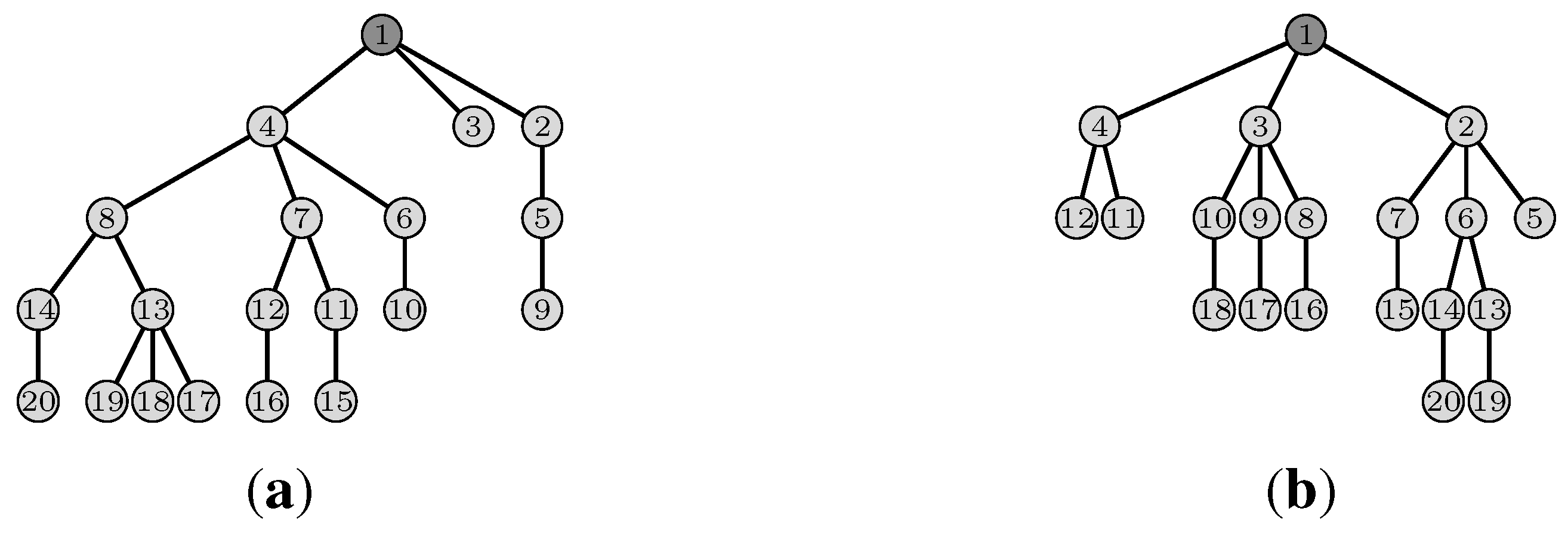
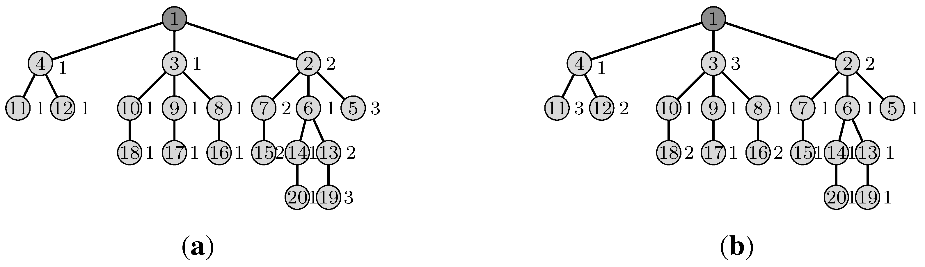
- A configuration is denoted when the optimal number of slots is imposed by the most demanding subtree rooted at a sink child, i. Its demand is equal to .
- A configuration is denoted when the optimal number of slots depends only on the total number of demands and . It is equal to . Notice that a configuration corresponds to a Capacitated Minimal Spanning Tree, where each branch has a total demand for slots, [12].
3.3.5. Specific Cases: Sink with a Single Radio Interface or Homogeneous Demands
3.4. MODESA Algorithm
- Any node has a dynamic priority. The priority is equal to , where is the number of packets the node has in its buffer at the current iteration. is the total number of packets the parent of the node has to receive in a cycle. The idea behind this heuristic is to reduce the number of buffered packets by favoring nodes that have packets to transmit to a parent with a high number of packets to receive.
- Nodes compete for the current time slot if and only if they have data to transmit.
- In addition to being allowed to transmit in a slot, a node and its parent must have an available interface.
- For any slot, the first scheduled node is the node with the highest priority among all the nodes that have data to transmit. If several nodes have the same priority, MODESA chooses the node with the smallest identifier. The selected node is scheduled on the first available channel, c.
- Any competing node can be scheduled in the current time slot on channel c if and only if it does not interfere with nodes already scheduled on channel c in this slot.
- Conflicting nodes that interfere with nodes already scheduled in this slot are scheduled on a different channel, if one is available. Otherwise, in a next slot.
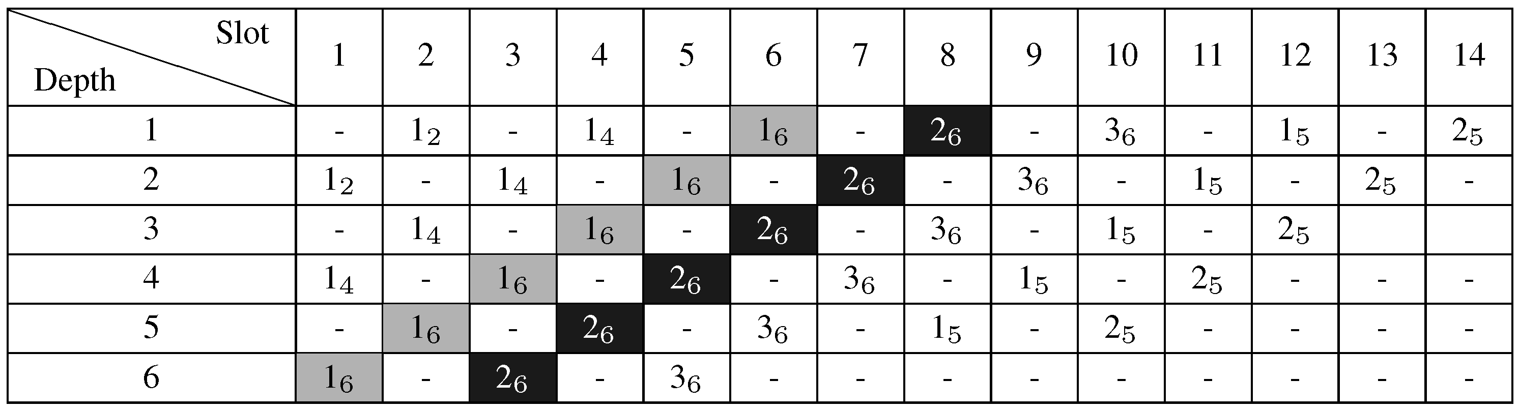
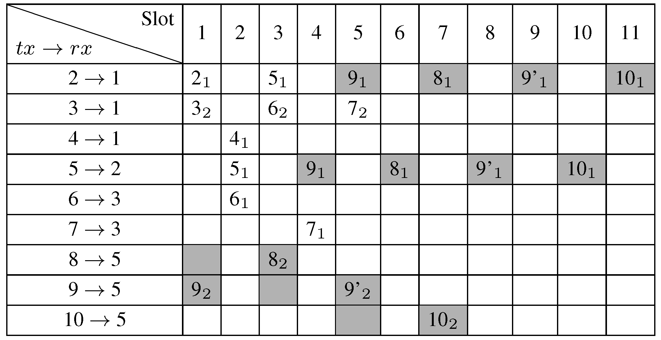
3.5. Illustrative Example

4. Adaptive Multichannel Slot Assignment
4.1. Definitions
4.2. Assumptions
- alarms have the highest priority,
- retransmissions of regular messages have medium priority,
- regular messages have the lowest priority.
4.3. Model

| Inputs | |
| set of links in the topology | |
| set of nodes in the topology | |
| set of available channels | |
| number of interfaces of the node, v | |
| set of nodes conflicting with v | |
| number of bonus slots requested by node, n | |
| activity of the link e in time slot, t, on channel, c, | |
| Variables | |
| utility of slot, t | |
| number of slots needed to transmit over link, e, the additional packets generated by node, n | |
| assignment of bonus slot, t, to link, e, on channel, c, | |
4.4. Theoretical Bounds on the Number of Extra Slots for a Raw Data Convergecast
| = | if is even, | ||
| = | otherwise, |
| = | if is even, | ||
| = | otherwise, |
4.5. AMSA: Proposed Solution
4.5.1. Principles
4.5.2. AMSA Algorithm
- Any node requesting a bonus slot has a static priority, which is equal to , where depicts the depth of a node, u, in the convergecast tree and is the number of requested bonus slots (see line 6 of Algorithm 1). This priority favors nodes requesting a longer slot path or a higher number of bonus slots. The goal is to minimize the number of extra slots. The length of a slot path is given by the depth of the requesting node. Since AMSA allocates slots per slot path, scheduling the longer path first helps AMSA to complete the schedule earlier.
- Nodes having bonus requests are sorted according to their priorities: the node with the highest priority is selected first (see line 7 of Algorithm 1).
- The sink serves the bonus requests from the selected node, assigning one bonus slot to the whole path to the sink (see lines 9 to 34 of Algorithm 1).
- To be allowed to transmit in a slot, both the selected node node and its parent should have an available radio interface (see line 12 of Algorithm 1). Consequently, AMSA searches for the first slot where this condition is met.
- AMSA searches for the first channel where this node does not conflict with the already transmitting nodes on the same channel. Hence, a node is scheduled in the earliest possible slot (see lines 13 to 22 of Algorithm 1).
- Any ordinary node, u, maintains a counter, , that corresponds to the number of bonus slots it will request: see Algorithm 2.
| Algorithm 1 AMSA algorithm for the sink. |
|
| Algorithm 2 AMSA algorithm for any ordinary node, u. |
|
4.5.3. Discussions
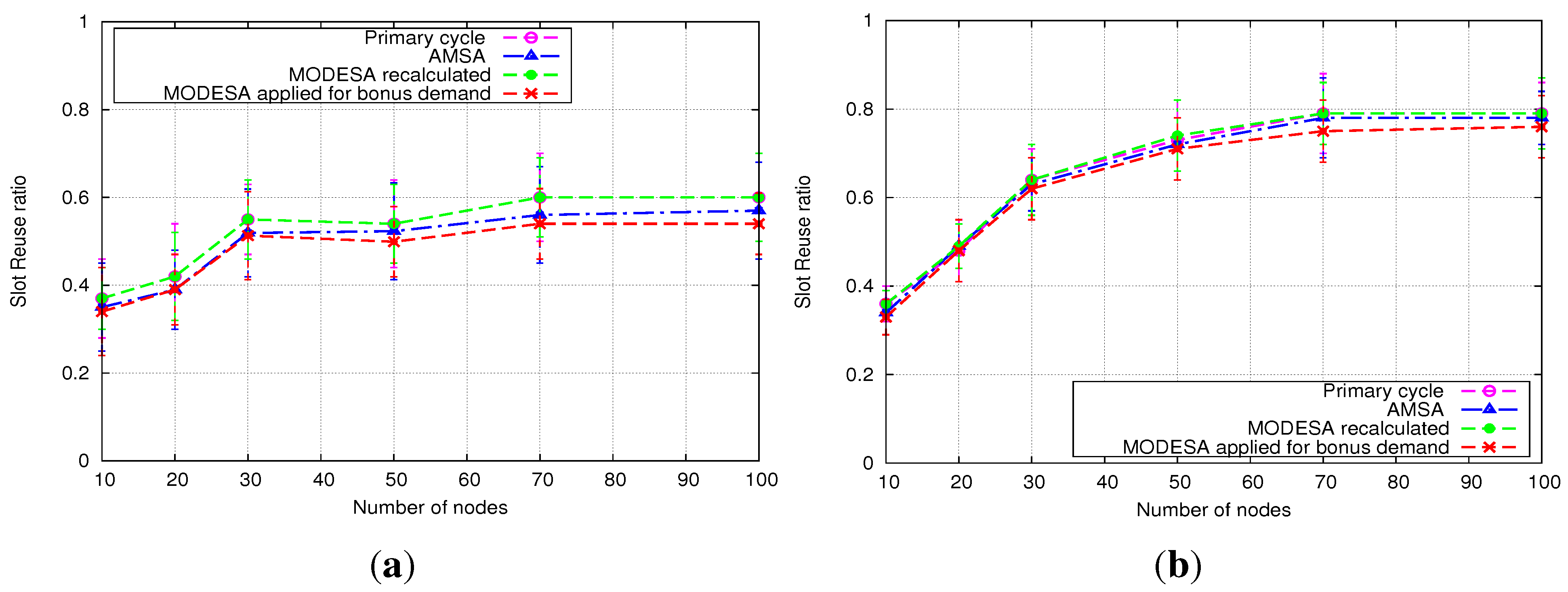
- spatial reuse: AMSA does not systematically require additional slots, due to its opportunistic behavior. Indeed, it takes advantage of spatial reuse to fill the slots with the new demands and, if that is impossible, adds a minimum number of slots. In both cases, AMSA ensures that (1) the number of available radio interfaces allows the transmission from the node considered to its parent and (2) no two conflicting nodes will transmit in the same slot on the same channel.
- a unique algorithm that can be used both for retransmissions at the MAC level and new transmission needs at the application level. The same algorithm is able to adapt to both application or MAC changes in their transmission needs. Furthermore, AMSA assigns a whole slot path. Indeed, each time a node requests an additional slot, the whole slot path corresponding to the slot sequence needed to reach the sink will, if possible, be granted.
- optimized retransmissions and a simpler implementation: on the one hand, we notice that with AMSA, only the sequence of slots starting with the transmitter that has not received the acknowledgment is allocated. On the other hand, the implementation is made simpler, because on any node, at any time, there is at most one pending message waiting for its acknowledgment.
- an energy efficient convergecast: Firstly, it minimizes the number of slots which is crucial from an energy point of view, as it allows nodes to sleep to save energy. On the other hand, conflict avoidance on the bonus and primary slots avoids collisions and, hence, contributes also to saving energy.
| AMSA | MODESA recalculated | ||
|---|---|---|---|
| Priority | nodes involved | only nodes requesting bonus slots | all nodes |
| when it is computed | once at the beginning of the algo | at the beginning of any slot | |
| Computation of the slot assigned to the highest priority node | any slot from the first one up to the current one | the current one | |
| Number of transmissions to schedule | |||
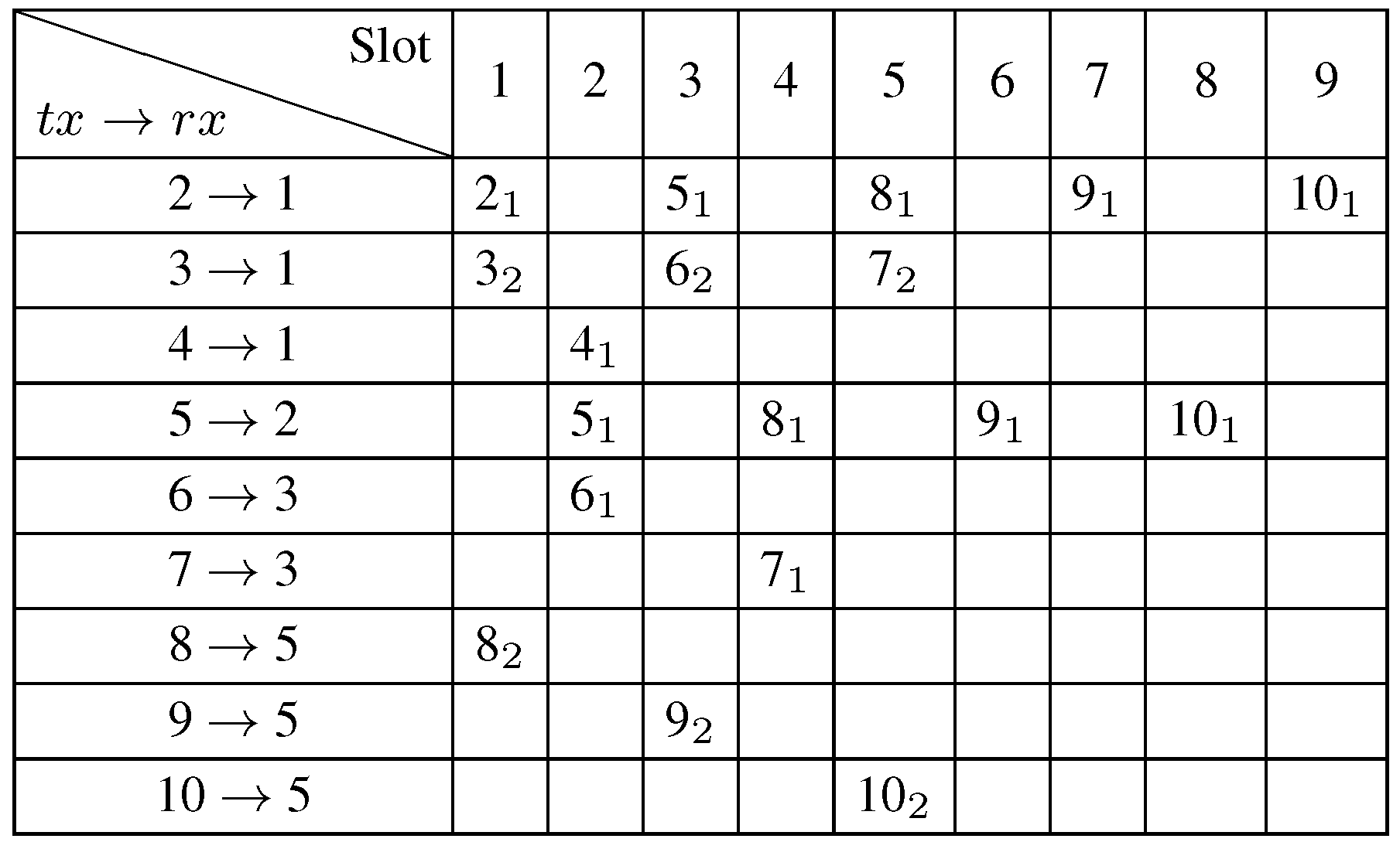
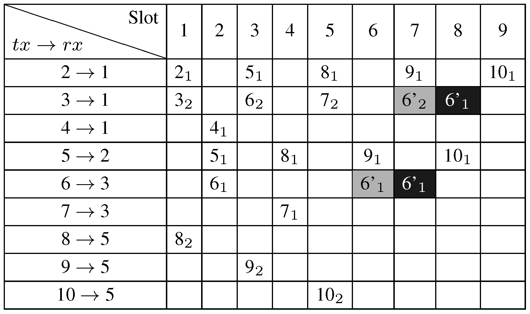
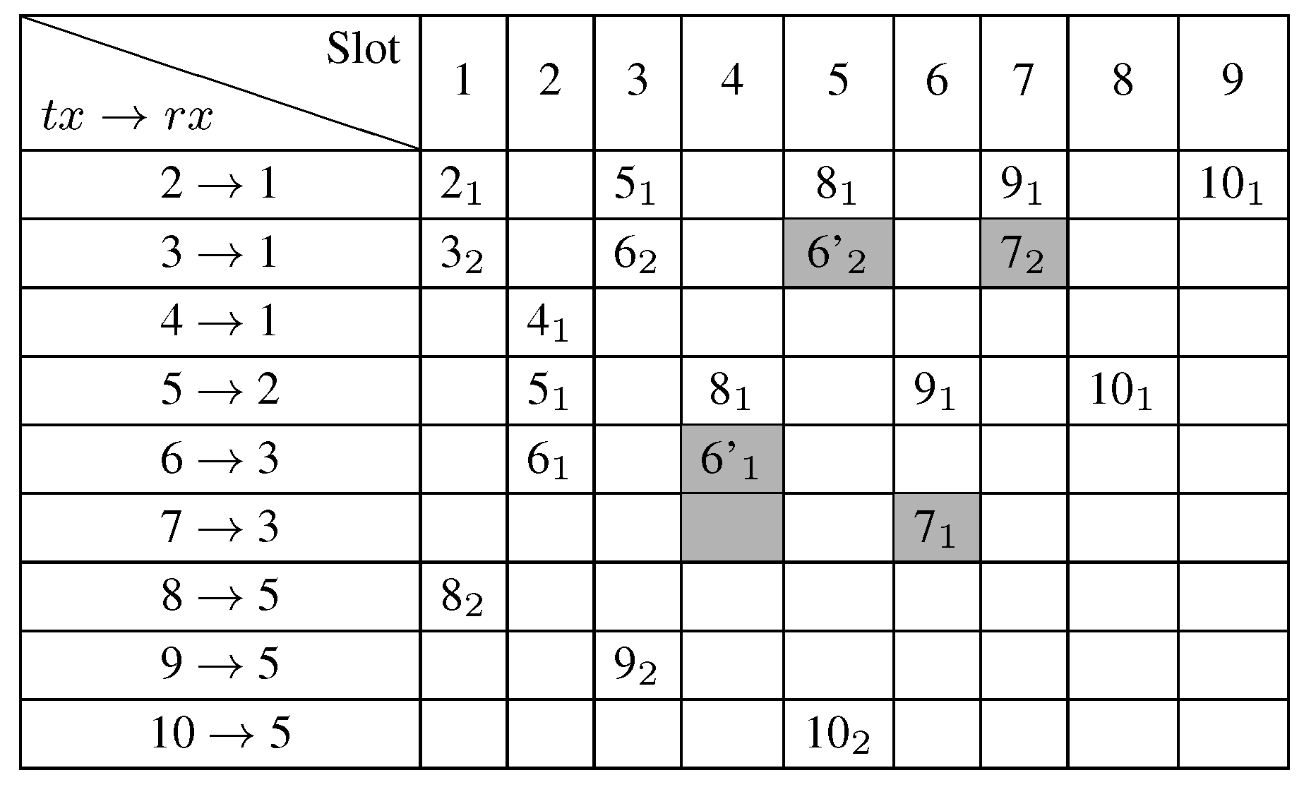
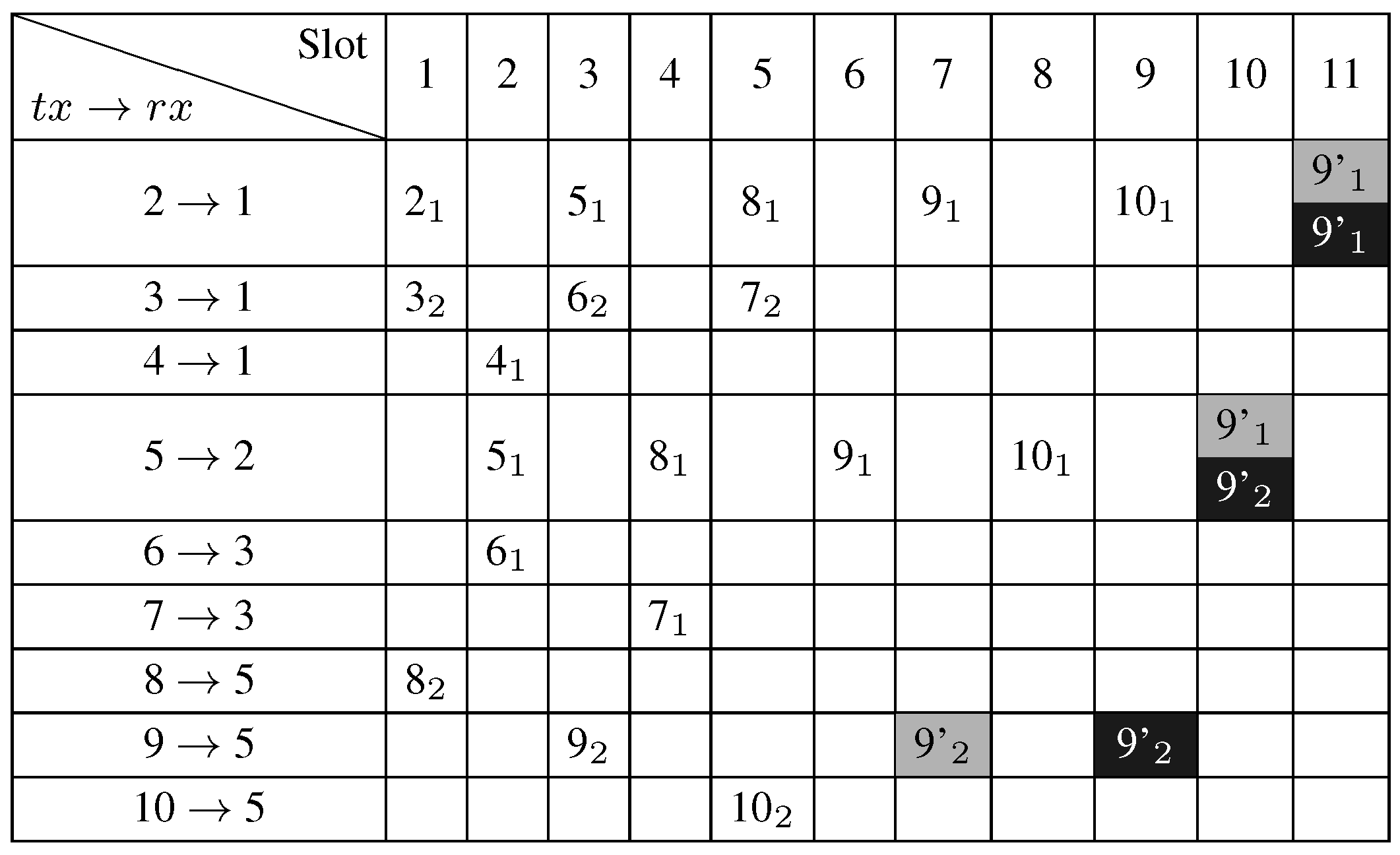
4.6. Illustrative Example


5. Performance Evaluation
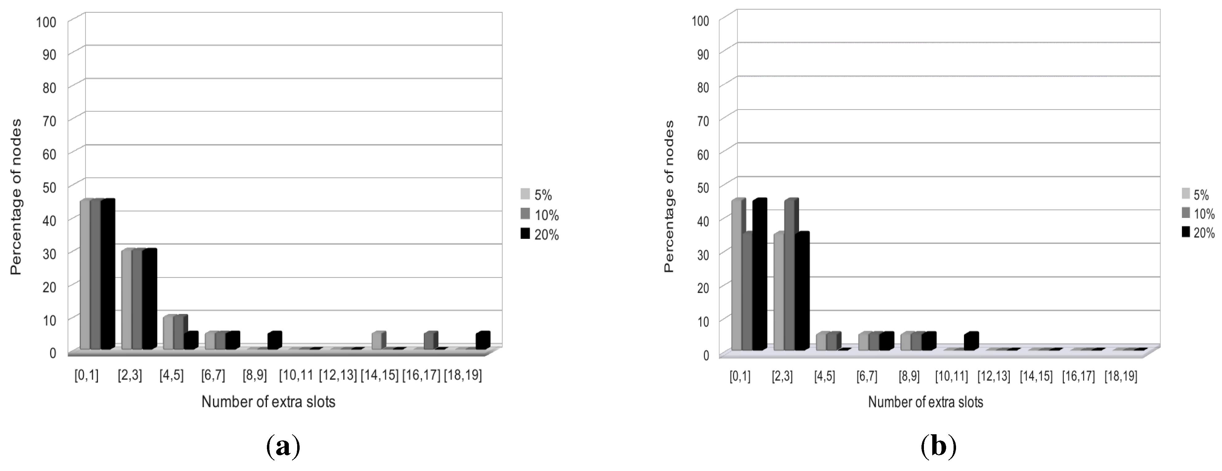
5.1. Retransmission Oriented Experiments
5.1.1. Homogeneous Initial Demands

5.1.2. Heterogeneous Initial Demands

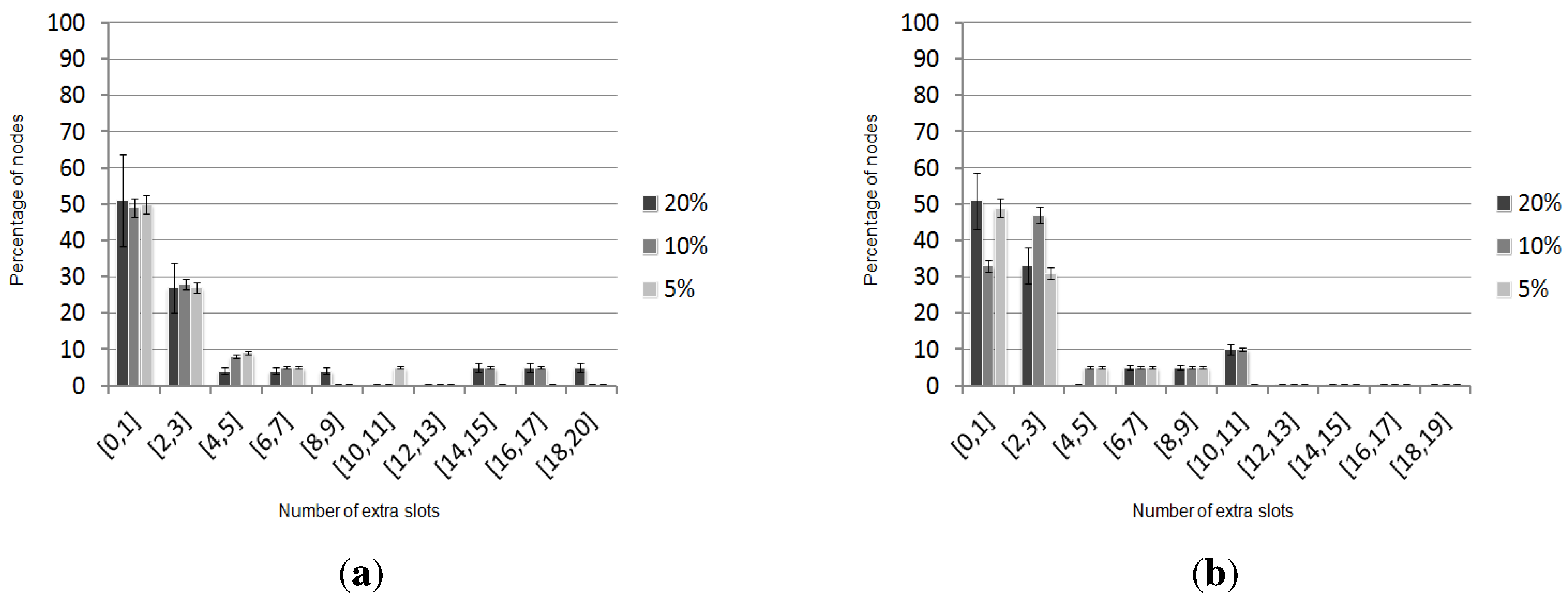
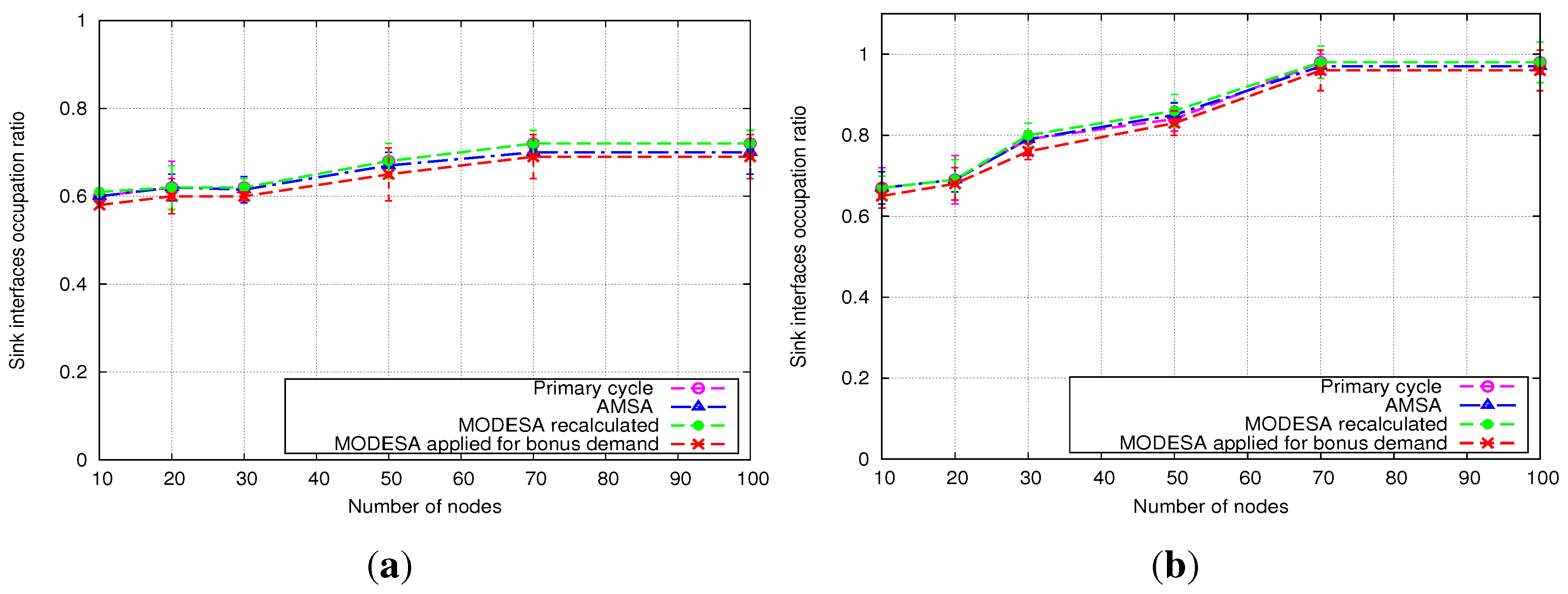
5.2. Temporary Change in the Application Needs-Oriented Experiments
5.2.1. Homogeneous Initial Demands

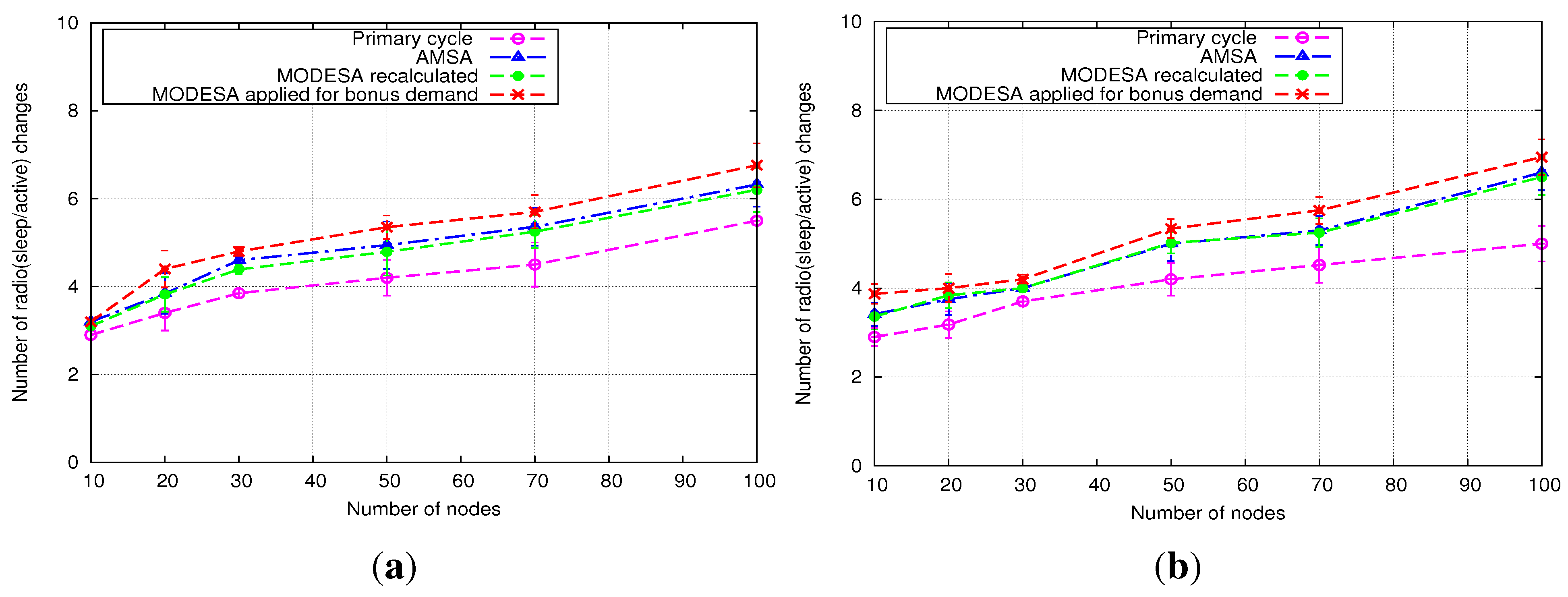
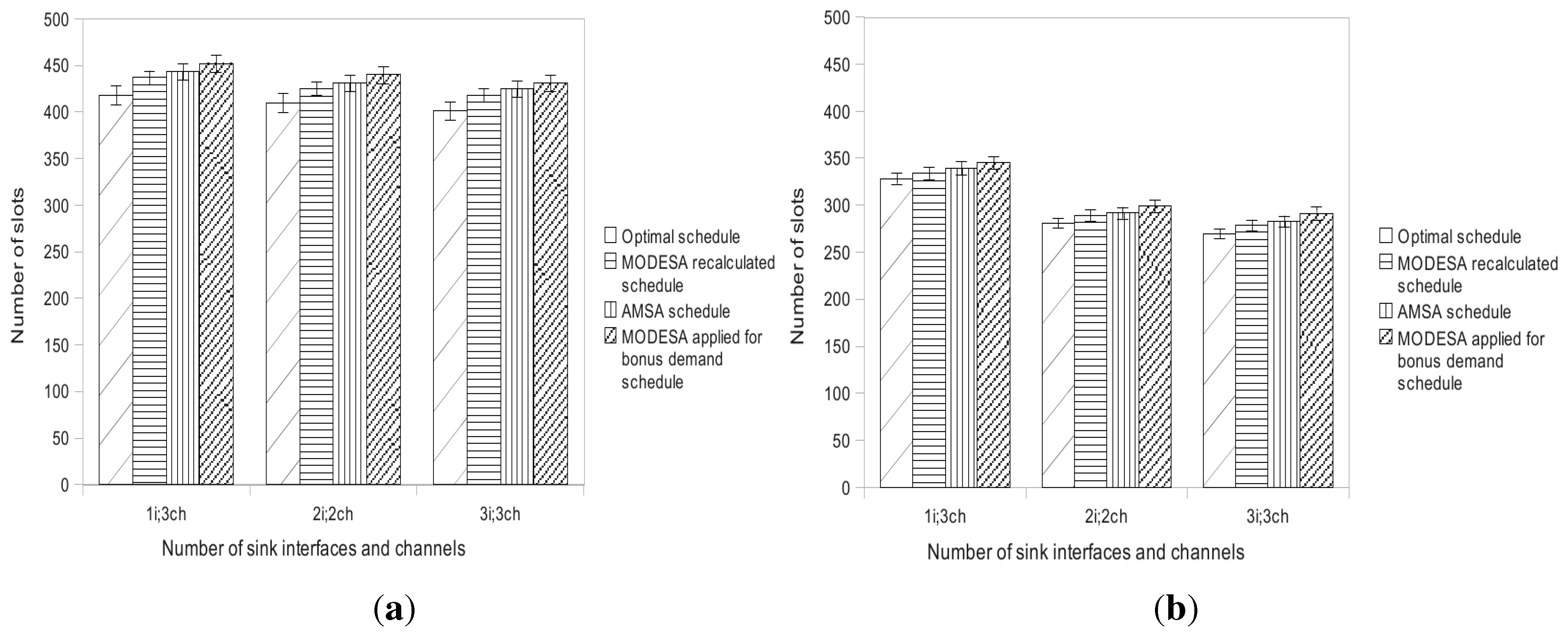
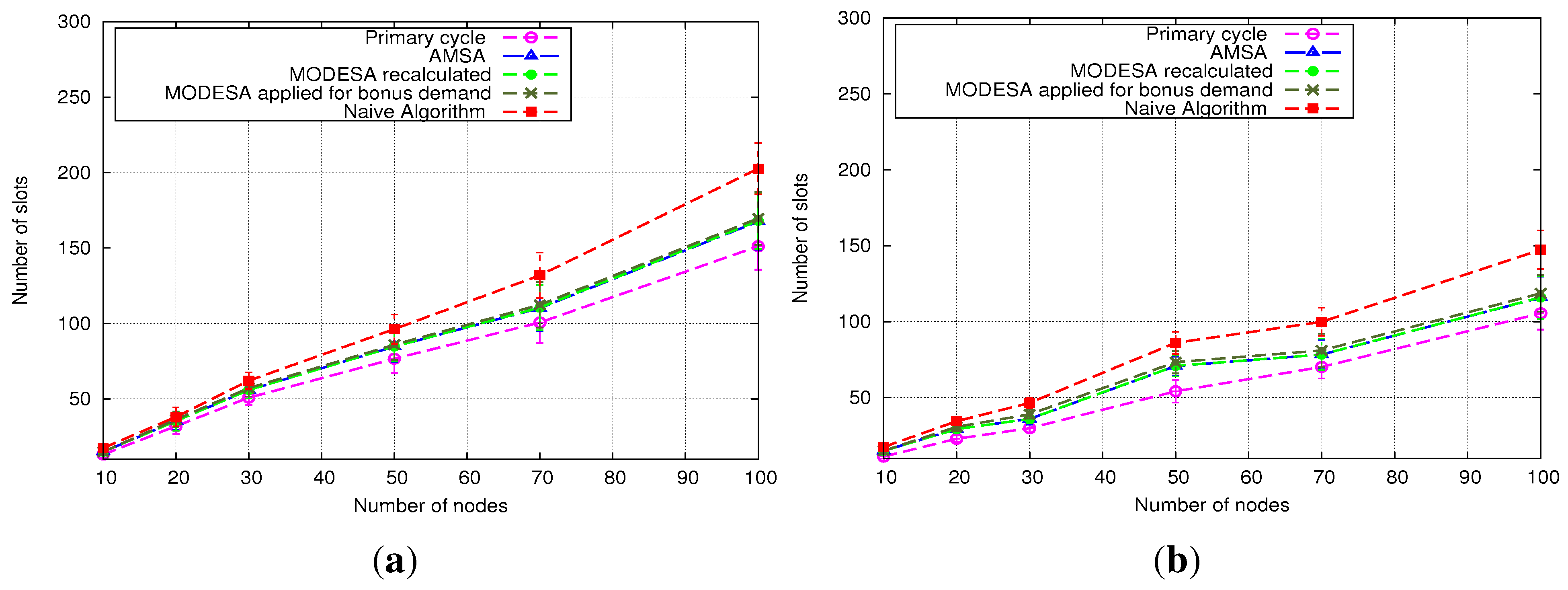
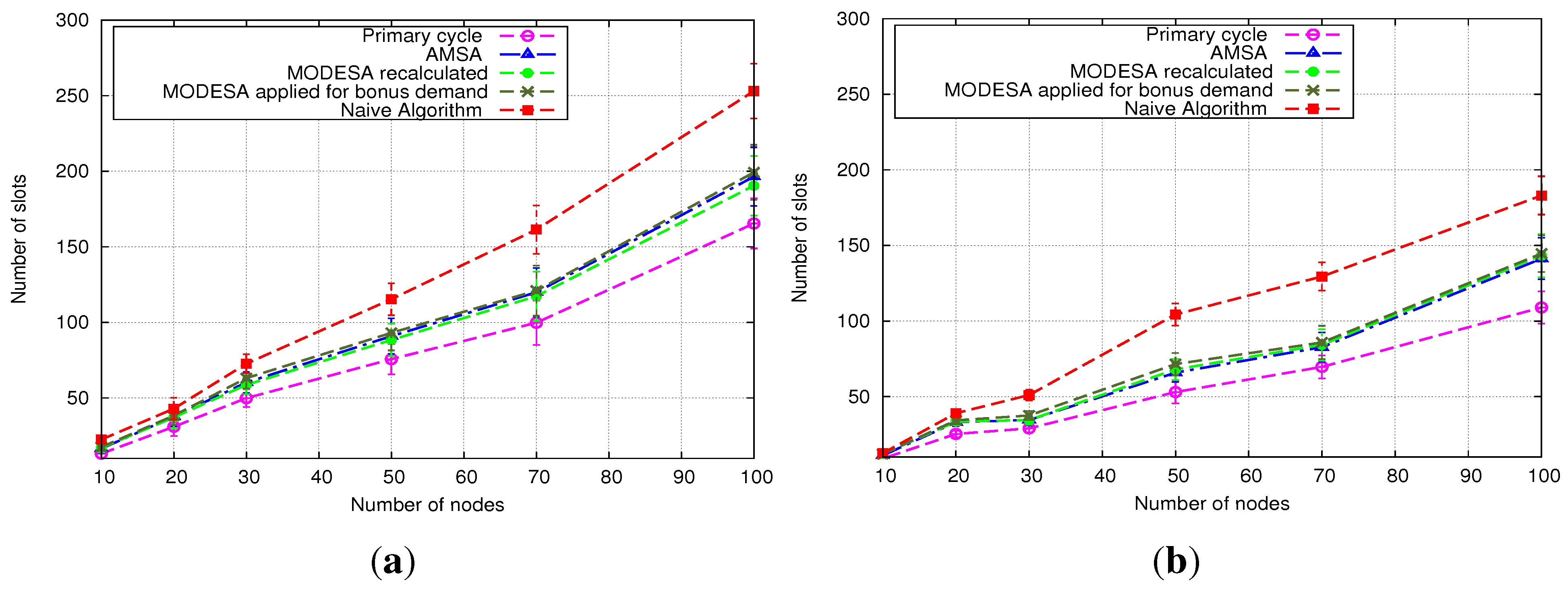
- MODESA recalculated: MODESA is run taking into account both initial and bonus demands.
- MODESA applied for bonus demand: MODESA is run in the primary schedule and also in the complementary schedule to schedule bonus demands.
- Naive Algorithm: assigns each extra slot exclusively to one transmitter.


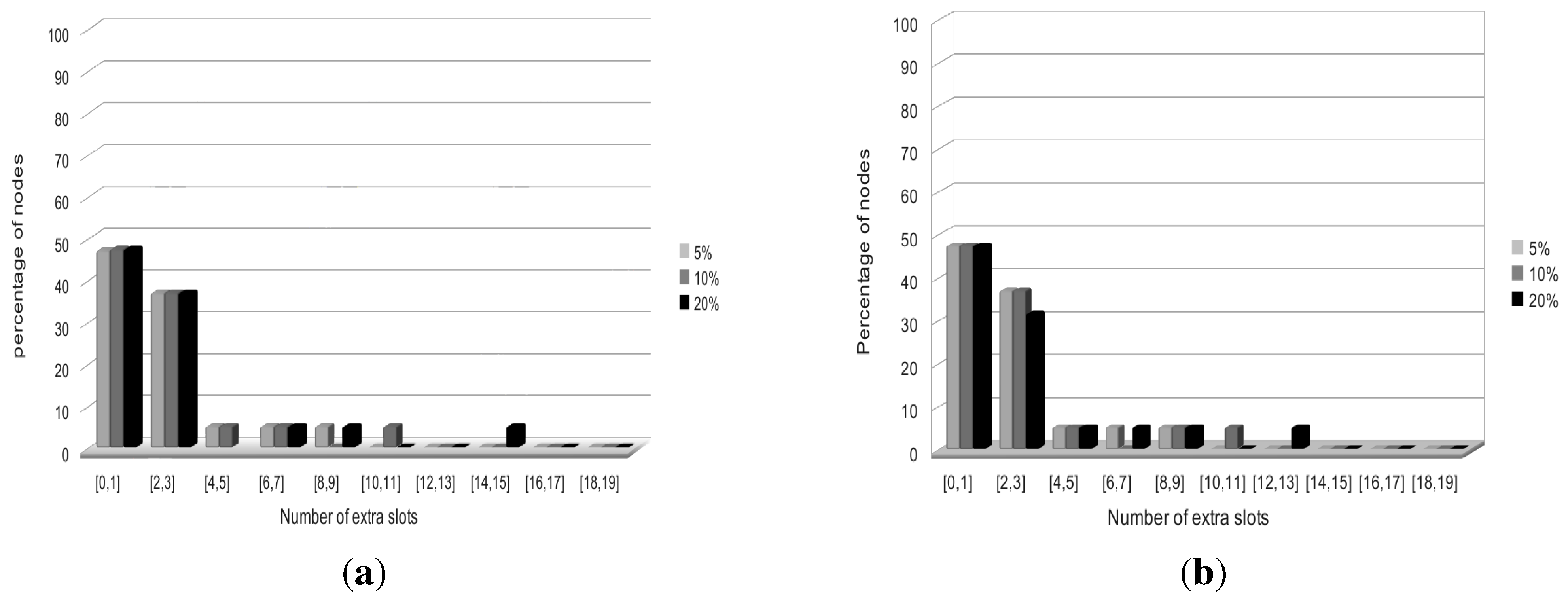
5.2.2. Heterogeneous Initial Demands


6. Conclusion
Acknowledgments
Conflict of Interest
References
- Ghosh, A.; Incel, O.D.; Kumar, A.; Krishnamachari, B. Multi-Channel Scheduling Algorithms for Fast Aggregated Convergecast in Sensor Networks. In Proceedings of the 6th IEEE International Conference on Mobile Adhoc and Sensor Systems (MASS), Macau, China, 12–15 October 2009.
- Soua, R.; Minet, P.; Livolant, E. MODESA: An Optimized Multichannel Slot Assignment for Raw Data Convergecast in Wireless Sensor Networks. In Proceedings of the 31 International Performance Computing and Communications Conference (IPCCC), Austin, TX, USA, 1–3 December 2012.
- Zhang, H.; Soldati, P.; Johansson, M. Optimal Link Scheduling and Channel Assignment for Convergecast in Linear WirelessHART Networks. In Proceedings of the International Conference on Modeling and Optimization in Mobile, Ad Hoc, and Wireless Networks (WiOPT’09), Seoul, Korea, 23–25 June 2009.
- Wu, Y.; Stankovic, J.; He, T.; Lin, S. Realistic and Efficient Multi-channel Communications in Wireless Sensor Networks. In Proceedings of the International Conference on Computer Communications, INFOCOM’08, Phoenix, AZ, USA, 15–17 April 2008.
- Incel, O.D.; Gosh, A.; Krishnamachari, B.; Chintalapudi, K. Fast data collection in tree-based wireless sensor networks. IEEE Trans. Mob. Comput. 2012, 1, 86–99. [Google Scholar]
- Cui, M.; Yin, J.; Nie, J.; Zhang, J.; Cao, Y. An Evolutionary Dynamic Slot Assignment Based on P-TDMA for Mobile Adhoc Network. In Proceedings of the 11th IEEE Singapore International Conference on Communication Systems (ICCS), Guangzhou, China, 19–21 November 2008.
- Gexin, P.; Shengli, X.; Caiyun, C. A collision-avoid dynamic slots assignment algorithm based on fixed TDMA. China Inf. Secur. 2005, 11, 115–120. [Google Scholar]
- Gobriel, S.; Mosse, D.; Cleric, R. TDMA-ASAP: Sensor Network TDMA Scheduling with Adaptive Slot-Stealing and Parallelism. In Proceedings of the 29th IEEE International Conference on Distributed Computing Systems (ICDCS), Montreal, QC, Canada, 22–26 June 2009.
- Yackovich, J.; Mosse, D.; Rowe, A.; Rajkumar, R. Making WSN TDMA Practical: Stealing Slots Up and Down the Tree. In Proceedings of the 17th IEEE International Conference on Embedded and Real-Time Computing Systems and Applications(RTCSA), Toyama, Japan, 28–31 August 2011.
- Kanzaki, A.; Hara, T.; Nishio, S. On a TDMA Slot Assignment Considering the Amount of Traffic in Wireless Sensor Networks. In Proceedings of the International Conference on Advanced Information Networking and Applications Workshops (WAINA), Bradford, UK, 26–29 May 2009.
- Tselishchev, Y.; Libman, L.; Boulis, A. Energy-efficient Retransmission Strategies Under Variable TDMA Scheduling in Body Area Networks. In Proceedings of the 36th IEEE Conference on Local Computer Networks (LCN), Bonn, Germany, 4–7 October 2011.
- Papadimitriou, C.H. The complexity of the capacitated tree problem. Networks 1978, 8, 217–230. [Google Scholar] [CrossRef]
- GLPK (GNU Linear Programming Kit). Available online: http://www.gnu.org/software/glpk/ (accessed on 10 May 2013).
- GNU Octave. Available online: http://www.gnu.org/software/octave/ (accessed on 15 January 2013).
© 2013 by the authors; licensee MDPI, Basel, Switzerland. This article is an open access article distributed under the terms and conditions of the Creative Commons Attribution license (http://creativecommons.org/licenses/by/3.0/).
Share and Cite
Soua, R.; Livolant, E.; Minet, P. An Adaptive Strategy for an Optimized Collision-Free Slot Assignment in Multichannel Wireless Sensor Networks. J. Sens. Actuator Netw. 2013, 2, 449-485. https://doi.org/10.3390/jsan2030449
Soua R, Livolant E, Minet P. An Adaptive Strategy for an Optimized Collision-Free Slot Assignment in Multichannel Wireless Sensor Networks. Journal of Sensor and Actuator Networks. 2013; 2(3):449-485. https://doi.org/10.3390/jsan2030449
Chicago/Turabian StyleSoua, Ridha, Erwan Livolant, and Pascale Minet. 2013. "An Adaptive Strategy for an Optimized Collision-Free Slot Assignment in Multichannel Wireless Sensor Networks" Journal of Sensor and Actuator Networks 2, no. 3: 449-485. https://doi.org/10.3390/jsan2030449
APA StyleSoua, R., Livolant, E., & Minet, P. (2013). An Adaptive Strategy for an Optimized Collision-Free Slot Assignment in Multichannel Wireless Sensor Networks. Journal of Sensor and Actuator Networks, 2(3), 449-485. https://doi.org/10.3390/jsan2030449