Article

DAR-MDE: Depth-Attention Refinement for Multi-Scale Monocular Depth Estimation

1
Department of Computer Engineering and Mathematics, Universitat Rovira i Virgili, 43007 Tarragona, Spain
2
Department of Electrical Engineering, Assiut University, Assiut 71516, Egypt
*
Authors to whom correspondence should be addressed.
J. Sens. Actuator Netw. 2025, 14(5), 90; https://doi.org/10.3390/jsan14050090
Submission received: 16 June 2025 / Revised: 2 August 2025 / Accepted: 15 August 2025 / Published: 1 September 2025

Abstract

Monocular Depth Estimation (MDE) remains a challenging problem due to texture ambiguity, occlusion, and scale variation in real-world scenes. While recent deep learning methods have made significant progress, maintaining structural consistency and robustness across diverse environments remains difficult. In this paper, we propose DAR-MDE, a novel framework that combines an autoencoder backbone with a Multi-Scale Feature Aggregation (MSFA) module and a Refining Attention Network (RAN). The MSFA module enables the model to capture geometric details across multiple resolutions, while the RAN enhances depth predictions by attending to structurally important regions guided by depth-feature similarity. We also introduce a multi-scale loss based on curvilinear saliency to improve edge-aware supervision and depth continuity. The proposed model achieves robust and accurate depth estimation across varying object scales, cluttered scenes, and weak-texture regions. We evaluated DAR-MDE on the NYU Depth v2, SUN RGB-D, and Make3D datasets, demonstrating competitive accuracy and real-time inference speeds (19 ms per image) without relying on auxiliary sensors. Our method achieves a δ < 1.25 accuracy of 87.25% and a relative error of 0.113 on NYU Depth v2, outperforming several recent state-of-the-art models. Our approach highlights the potential of lightweight RGB-only depth estimation models for real-world deployment in robotics and scene understanding.

1. Introduction

Estimating depth from monocular images has emerged as a critical task in computer vision, with broad applications in autonomous driving, robotics, augmented reality, and scene understanding [1,2]. Unlike stereo or multi-view setups, monocular depth estimation relies on a single image, making it a cost-effective and flexible solution. However, inferring depth from a single viewpoint remains inherently ambiguous and challenging due to factors such as lighting variations, occlusions, and scene complexity [3].
Recent advances in deep learning have significantly enhanced the performance of monocular depth estimation methods. Convolutional Neural Networks (CNNs) and transformer-based architectures have shown strong capabilities in capturing both local texture details and global contextual information [3,4]. Techniques such as multi-scale feature fusion, self-attention mechanisms, and uncertainty modeling have further improved the accuracy and robustness of depth predictions [5,6]. Additionally, physics-based modeling methods such as dehazing-inspired frameworks have contributed to more effective scene understanding under challenging visual conditions [7].
Additionally, self-supervised and semi-supervised learning approaches have gained traction by reducing the dependence on dense ground-truth annotations and enabling effective training with large-scale unlabeled data [4,8]. The integration of auxiliary modalities such as infrared or LiDAR data through multimodal fusion has also demonstrated promising results, particularly in challenging scenarios [9].
Despite these advancements, achieving a balance between real-time performance and prediction accuracy remains an open challenge, especially in complex and diverse environments. Current research continues to explore lightweight architectures, attention-guided refinement modules, and uncertainty-aware strategies to address these limitations [8,10,11].
While many existing methods achieve high quantitative accuracy, they still struggle to consistently capture scale variability and preserve sharp structural edges, especially near object discontinuities or in scenes with mixed-size objects [12]. Industrial and robotic applications demand depth maps that are not only globally accurate but also robust across scales and sensitive to fine-grained geometric details. This motivates us to develop a model architecture that explicitly aggregates multi-scale context and focuses attention on key structural regions in order to better handle diverse environments ranging from cluttered indoor scenes to open outdoor landscapes.
Recently, the advancement of deep neural networks has made it possible to easily infer accurate depth information from a single image [13,14,15]. Monocular depth estimation systems can predict depth better than humans. Some remaining issues, such as the need for a large amount of training data and domain adaptation, must still be appropriately addressed [16]. Furthermore, research indicates that industrial companies are looking to reduce costs while improving the performance of such systems. Although many methods for estimating depth from a single image have been proposed, there is still room to improve currently proposed models in terms of accuracy, robustness, and reduced complexity.
Although depth maps are fairly reliable overall, the estimates around object discontinuities are far from satisfactory [17]. Furthermore, the depth information of small and tiny objects is often incorrectly estimated. This is because the convolutional operator naturally aggregates features across object discontinuities, resulting in smooth transitions rather than sharp edges [17]. To address this issue, we propose a novel deep learning model explicitly designed to exploit feature aggregation at different image scales. In addition, we propose using an attention module to provide an additional focus on objects, noting their specific importance in the scene in order to obtain more precise depth maps.
Many existing monocular depth estimation methods rely on fixed-scale feature extraction or single-scale representations, limiting their ability to capture depth cues for objects at varying sizes and distances. This results in poor handling of scale variations. Furthermore, traditional architectures and loss functions often smooth depth predictions, causing blurry edges and loss of fine structural details around object boundaries. To address these challenges, our proposed Multi-Scale Feature Aggregation (MSFA) network explicitly aggregates features at multiple scales, combining coarse global context with fine local details to improve scale robustness. In addition, the Refining Attention Network (RAN) employs an attention mechanism to selectively focus on spatially salient regions, particularly object boundaries, preserving sharp edges by adaptively weighting features critical for depth discontinuities. These modules enable our model to better handle scale variations and maintain clear structural edges compared to conventional methods.
Consequently, this work proposes an approach that uses an autoencoder with a Multi-Scale Feature Aggregation and Refining Attention Network modules to improve prediction accuracy and generate a more accurate dense depth image under different conditions for depth estimation from the complete scene. Our approach could be considered an extension of the works proposed in [18,19,20], which are identical to how we utilize the Multi-Scale Feature Aggregation and Refining Attention Depth Network to generate depth maps from monocular images. The proposed model consists of an autoencoder network incorporating a Multi-Scale Feature Aggregation network, a Refining Attention Depth network, and a multi-scale loss function. These elements have been combined in a single pipeline to accurately generate dense depth maps from a single camera. Our approach focuses on estimating the depth information of the object regardless of its scale in order to obtain a depth map that is robust to changes in scale or viewpoint. Our model can also estimate depth maps for indoor and outdoor environments. Furthermore, it produces results with high precision and a reasonable computational cost compared to current state-of-the-art methods. Figure 1 shows an overview of the proposed network model. The main contributions of this work are clearly summarized as follows:
  • We develop a depth estimation framework that integrates a Multi-Scale Feature Aggregation (MSFA) module to enable robust learning across objects of varying sizes and scene perspectives.
  • We incorporate a Refining Attention Network (RAN) module that selectively emphasizes structurally important regions by learning the relationship between coarse depth probabilities and local feature maps.
  • We introduce a multi-scale loss strategy based on curvilinear saliency that enforces depth consistency at multiple resolutions, leading to sharper boundaries and better small object representation.
  • We validate our approach extensively on both indoor (NYU Depth v2, SUN RGB-D) and outdoor (Make3D) datasets, demonstrating superior generalization without reliance on additional sensors such as LiDAR or infrared. The results highlight its light weight and applicability for monocular scenarios.
The rest of this paper is structured as follows: related work is summarized in Section 2; the proposed methodology for depth estimation is described in Section 3; the experimental findings and performance are presented in Section 4; finally Section 5 concludes this paper.

2. Related Work

This section presents an overview of the current research on depth estimation, multi-scale networks, and refining attention networks.

2.1. Depth Estimation

Recently, there has been growing interest in monocular depth estimation due to its potential applications in fields such as autonomous driving and robotics. However, determining depth information from a single image can be challenging, as it requires stereo visual cues provided by multiple cameras. Monocular depth estimation methods use deep learning techniques such as Convolutional Neural Networks (CNNs) to learn how to map from the image and depth domains. Various papers have proposed these methods, such as [21,22].
In [21], the authors proposed a generative adversarial model for estimating depth from a single monocular image. The model included a two-stage convolutional network as a generator to predict global and local structures of the depth image. Training was based on an adversarial discriminator which differentiated between real and generated depth images. This model allows for more accurate and structure-preserving depth prediction from a single image. In [23], the authors proposed using multi-scale information to determine depth from single images. Four CNN architectures incorporating multi-scale features were studied and compared to a single-scale method. The results revealed that incorporating multi-scale features can increase accuracy and improve the quality of the depth maps. In turn, the authors of [24] proposed a deep learning model to estimate depth maps of objects in single images, which they then used to predict the 3D pose of the object. The proposed model comprised two autoencoder networks based on a Generative Adversarial Neural network (GAN). A limitation of this model is that it assumes a cross-domain training procedure for 3D CAD models based on objects appearing in real photographs rather than for the complete scene.
Some works have tried to improve model performance by capturing cross-task contexts, as in dense prediction. In [25], the authors presented a new depth estimation model that utilizes semantic segmentation to estimate depth from monocular images. The model creates a shared parameter structure that combines semantic segmentation and depth information and uses it as a guide to assist depth acquisition. It also employs a multi-scale feature fusion module to merge feature information from multiple layers of a neural network to produce high-resolution feature maps, improving the depth image’s quality by enhancing the semantic segmentation model. Likewise, the authors of [26] presented a multi-task learning model that combines the advantages of deformable CNNs and query-based transformers for dense prediction. The model has a simple and effective encoder–decoder architecture that comprises a deformable mixer encoder and a task-aware transformer decoder. The deformable mixer encoder employs a channel-aware mixing operator for communication among different channels and a spatial-aware deformable operator for efficient sampling of more informative spatial locations. The task-aware transformer decoder comprises a task interaction block that captures task interaction features via self-attention and a task query block that leverages the information to generate task-specific features through a query-based transformer for corresponding task predictions.
Recent works continue to advance the field of monocular depth estimation through a variety of innovative strategies. In [1], the authors introduced a dual-attention network that integrated spatial and channel attention mechanisms to enhance the quality of depth predictions. In [6], a scale-aware deep network was proposed that adapts to varying depth levels across scenes by leveraging multi-scale modules. In [3], the authors explored transformer-based architectures to capture long-range dependencies, thereby improving the structural consistency of the estimated depth maps. The authors of [4] leveraged geometric constraints in a self-supervised setting, significantly reducing the reliance on labeled depth data while maintaining high accuracy.
In [27], a multi-scale adaptive feature fusion model was presented that dynamically combines features across scales to improve depth estimation performance. The authors of [5] introduced a Bayesian deep learning framework to quantify prediction uncertainty, enhancing reliability in safety-critical applications. For real-time deployment, ref. [8] developed lightweight networks that maintain competitive accuracy under computational constraints, while [9] investigated multimodal fusion by integrating monocular inputs with auxiliary sensor data such as infrared or LiDAR for increased robustness in complex environments. In [11], attention mechanisms were applied to sparse depth completion tasks, which can also be integrated into monocular depth pipelines for refinement. Lastly, ref. [28] proposed a hierarchical multi-scale approach that progressively refines depth predictions, resulting in enhanced resolution and structural coherence.

2.2. Multi-Scale Networks

Multi-scale networks have been widely used in image analysis. These networks are designed to capture both fine and coarse details of an image by processing the image at multiple scales. The multi-scale information is then used to estimate the critical features in the images. Regarding depth estimation, the multi-scale approach is motivated by the fact that the depth of an object in an image can vary at different scales, and a single-scale network may only capture some of the necessary depth information.
Recently, multi-scale networks have been proven effective in various monocular depth estimation methods [18,20,29]. In [20], the authors proposed a supervised monocular depth estimation network which employs a new architecture that includes local planar guidance layers. These layers establish an explicit link between internal feature maps and the desired depth prediction, improving the network training. The layers are incorporated at multiple stages during the decoding phase of the network. In turn, ref. [18] proposed a recurrent attention network for multi-scale depth estimation using RGB-D saliency detection. Their method uses residual connections to extract and combine information from RGB and depth streams for improved results. They also use depth cues and multi-scale contextual features to locate salient objects. A recurrent attention module is utilized for more accurate saliency results, while cascaded hierarchical feature fusion is used to improve the overall performance. The authors of [29] employed multi-level depth map estimators in the decoder part to learn scale-aware depth map context by utilizing context-aware features extracted from different scales. This approach helps to maintain object structure detail and generate sharp boundaries, particularly in complex environments.
Thus, multi-scale networks can make depth estimation more robust and accurate, especially in challenging scenarios such as low-texture areas and reflective surfaces. In this paper, we use the advantages of the multi-scale approach to improve the resulting model’s overall performance in estimating the depth information of the objects regardless of scale, making it more robust to scale variations.

2.3. Refining Attention Depth Network

Refining networks have been widely used in many applications to improve the accuracy and robustness of the predictions, including semantic segmentation, image-to-image translation, and depth estimation. Such refining networks are designed to refine the initial depth estimates obtained from an autoencoder network. The refining network can correct errors in the initial depth estimates or incorporate additional information such as stereo and temporal information. The refining attention depth can be applied in different ways, such as in [19,30]. The authors of [30] presented a refinement network in the form of a multi-path refinement network that uses long-range residual connections to enable high-resolution semantic segmentation. By utilizing fine-grained features from earlier convolutions, this allows for the refinement of deeper layers which capture high-level semantic features. The refinement network proposed in [30] employs residual connections and identity mapping for effective end-to-end training. Additionally, the authors introduced chained residual pooling, an efficient method for capturing rich background context. In this work, we exploit refining networks and apply them to allow the network to focus on the most informative regions of the image and refine the details of the depth map in those regions. For monocular depth estimation, ref. [19] introduced bidirectional attention modules that utilize the feed-forward feature maps and incorporate the global context to filter out ambiguity. This modeling approach addresses the need to integrate local and global information in convolutional networks. The structure of this mechanism derives from the strong conceptual foundation of neural machine translation, which presents a lightweight mechanism for adaptive computation control similar to the dynamic nature of recurrent networks.
Several works have also used refinement networks based on attention mechanisms, which allows the network to focus on specific regions of the input image. This can improve performance in challenging scenarios such as low-textured or uniform regions.
For instance, in [31] the authors proposed an Attentional Generative Adversarial Network (AttnGAN) for fine-grained text-to-image generation. This approach uses a novel attentional generative network to synthesize fine details in specific image regions along with a deep attentional multimodal similarity model to compute a fine-grained image-text matching loss for training the generator. Likewise, the authors of [32] proposed the Contextual Attention Refinement Network (CARNet), which uses the Contextual Attention Refinement Module (CARModule) to learn an attention vector that guides the fusion of low- and high-level features for improved segmentation accuracy. Additionally, the the semantic information is considered by introducing the Semantic Context Loss (SCLoss) into the overall loss function. In [33], the authors introduced KRAN (Knowledge Refining Attention Network) to improve recommendation performance by exploiting the characteristics of knowledge graphs. KRAN utilizes a traditional attention mechanism to extract more precise knowledge from the knowledge graph, then employs a refining mechanism to make the extraction process more efficient. The proposed mechanism first evaluates the relevance of an entity and its neighboring entities in the knowledge graph using attention coefficients. It then refines these coefficients using a ‘rich-get-richer’ principle, allowing the model to focus on highly relevant neighboring entities while reducing the noise caused by less relevant ones.
Our approach combines the advantages of multi-scale networks and refinement networks, achieving state-of-the-art performance to further boost the accuracy of monocular depth estimation.

3. Proposed Methodology

This section lays out the main steps of the proposed depth estimation model using monocular images and outlines the resources utilized in the course of our research. Figure 1 shows the architecture of the proposed approach, consisting of three main sub-models: the Autoencoder Network (Encoder E and Decoder D), Multi-Scale Feature Aggregation M S F A , and Refining Attention Network R A N . In addition, multi-scale loss functions M L are used while training the model. The first subsection presents the problem statement, while the following sections detail the proposed solution.

3.1. Problem Formulation

We can formulate the problem of depth estimation from a monocular image as follows. Given a monocular image X X of a scene captured by a single camera, the goal is to estimate a depth map Y Y which is a 2D representation of the distance from each pixel in the image to the camera. This can be formally defined as the function f : X Y that assigns elements from the domain X to elements in the co-domain Y . Our proposed model consists of four networks: the Encoder E ( X ) , Decoder D ( X ^ ) , Multi-Scale Feature Aggregation M S F A ( D ( X ^ ) ) , and Refining Attention Network R A N ( M S F A ( D ( X ^ ) ) ) .
Equations (1)–(5) explain the operation of the model’s workflow in the training and testing stages:
X ^ = E ( X ) ,
where X ^ stands for the features extracted from the encoder network E;
Y 1 = D ( X ^ ) ,
where Y 1 is the depth map extracted from the decoder network D;
S 1 , S 2 , S 3 , S 4 = D 1 ( X ^ ) , D 2 ( S 1 ) , D 3 ( S 2 ) , Y 1 ,
where e S i represents the scale features from decoder layers D i and Y 1 represents the depth maps from (2);
M = M S F A ( S 1 S 2 S 3 S 4 ) ,
where M is the concatenation of the features extracted in (3); and
Y ^ = R A N ( M , Y ) ,
where Y ^ is the final depth map extracted from R A N .
The modules of our architecture are grounded in well-established theoretical principles from the fields of computer vision and deep learning. The Multi-Scale Feature Aggregation (MSFA) module is inspired by scale-space theory [34], which emphasizes capturing structural details at multiple resolutions to enhance robustness in depth estimation. The Refining Attention Network (RAN) employs cosine similarity as a probabilistic attention mechanism, akin to those used in neural sequence modeling [35], enabling the model to dynamically emphasize depth-relevant regions. The curvilinear saliency loss function incorporates concepts from differential geometry, promoting edge-aware supervision by encouraging depth consistency along high-curvature boundaries. Together, these modules are designed with a strong theoretical justification, ensuring structural fidelity and improved generalization in monocular depth estimation.

3.2. Model Architecture

The proposed model architecture is based on three different networks coupled together. Each network can help the others to represent the key features of the depth image from the input image. First, we use the autoencoder network to learn a representation of an image while maintaining the important information needed during training to minimize the difference between the estimated depth and the ground truth depth. Second, the Multi-Scale Feature Aggregation (MSFA) network increases the ability of the first network to recognize objects regardless of size, making the model more robust to changes in scale or point of view. Third, the Refining Attention Network (RAN) is employed to help the model focus on dense depth regions of the monocular image and refine the details of the depth map in these regions. In addition, we use a multi-scale loss function that incorporates different depth scales from each block in the decoder part to compute the loss function, allowing the model to achieve a more accurate comparison of the ground truth and generated depth. This forces the autoencoder network to generate a more accurate dense depth image. The rest of this section describes the proposed system and its training procedure. The following subsections provide a more detailed description of the proposed network.

3.2.1. Autoencoder Network

Autoencoder networks are widely employed to learn compact representations of images that preserve critical structural details, making them effective for depth estimation tasks. Our autoencoder comprises an encoder E and a decoder D.
The encoder E receives an input RGB image and maps it into high-level feature representations. Specifically, we utilize SENet-154 [36] pretrained on ImageNet [37] for feature extraction. All layers of the SENet-154 backbone are used up to the final global pooling layer (before its classification head), ensuring that the entire hierarchical feature extraction capacity of the network contributes to the depth estimation process. The pretrained weights are directly employed without freezing, allowing end-to-end fine-tuning for our depth task.
Input RGB images are resized to 228 × 304 . The encoder generates progressively abstract feature maps through its four major residual stages, producing outputs of size 180 × 240 × 256 , 90 × 120 × 512 , 45 × 60 × 1024 , and finally 23 × 30 × 2048 . We apply a 1 × 1 convolution followed by batch normalization and ReLU activation to reduce channel dimensionality at the bottleneck.
The decoder D reconstructs depth maps using four deconvolution layers. Starting from 23 × 30 × 1024 (concatenated with a reduced bottleneck), each deconvolution halves the channel depth via 3 × 3 kernels. Between them, 2 × 2 bilinear upsampling [38] expands spatial resolution. ReLU activations are applied after each layer. At each stage, the decoder outputs are concatenated with skip connections from the corresponding encoder layers. The final output reaches 240 × 180 × 1 .
At the end of each decoder stage, multi-level depth estimators apply 3 × 3 convolutions to extract scale-aware context, as in [29], preserving both coarse structural context and fine object details. This ensures sharp depth boundaries even in geometrically complex scenes.

3.2.2. Multi-Scale Feature Aggregation Network

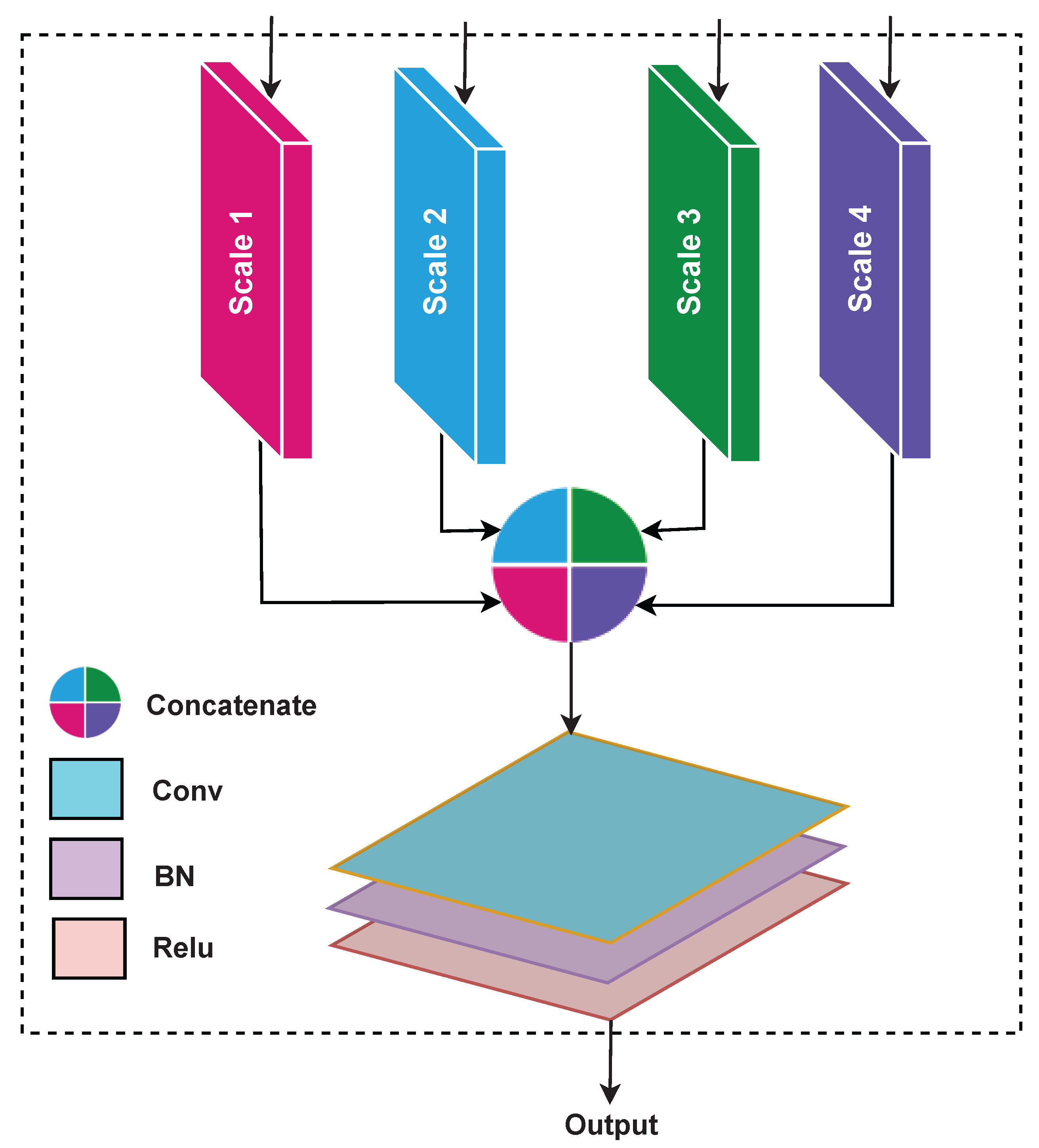
The Multi-Scale Feature Aggregation (MSFA) module combines information across different spatial resolutions to enhance robustness to object size variation and scene perspective. As illustrated in Figure 2, decoder outputs at multiple scales ( S 1 , S 2 , S 3 , S 4 ) are first upsampled to a common spatial resolution.
These upsampled features are then fused via channel-wise concatenation (as opposed to element-wise addition), forming a unified feature tensor that retains scale-specific information from each layer. This concatenated representation preserves distinct characteristics across scales and facilitates joint refinement.
The resulting feature map is passed through a 5 × 5 convolutional layer with 64 output channels, followed by batch normalization and ReLU activation. This produces the aggregated multi-scale feature representation, which serves as input to the subsequent Refining Attention Network (RAN) module.
This design is motivated by the need to address the limitations of fixed-scale feature extraction in existing methods, which struggle to capture depth cues across objects of varying sizes and distances. By aggregating multi-scale features, the MSFA module enhances the network’s ability to handle scale variation.

3.2.3. Refining Attention Network

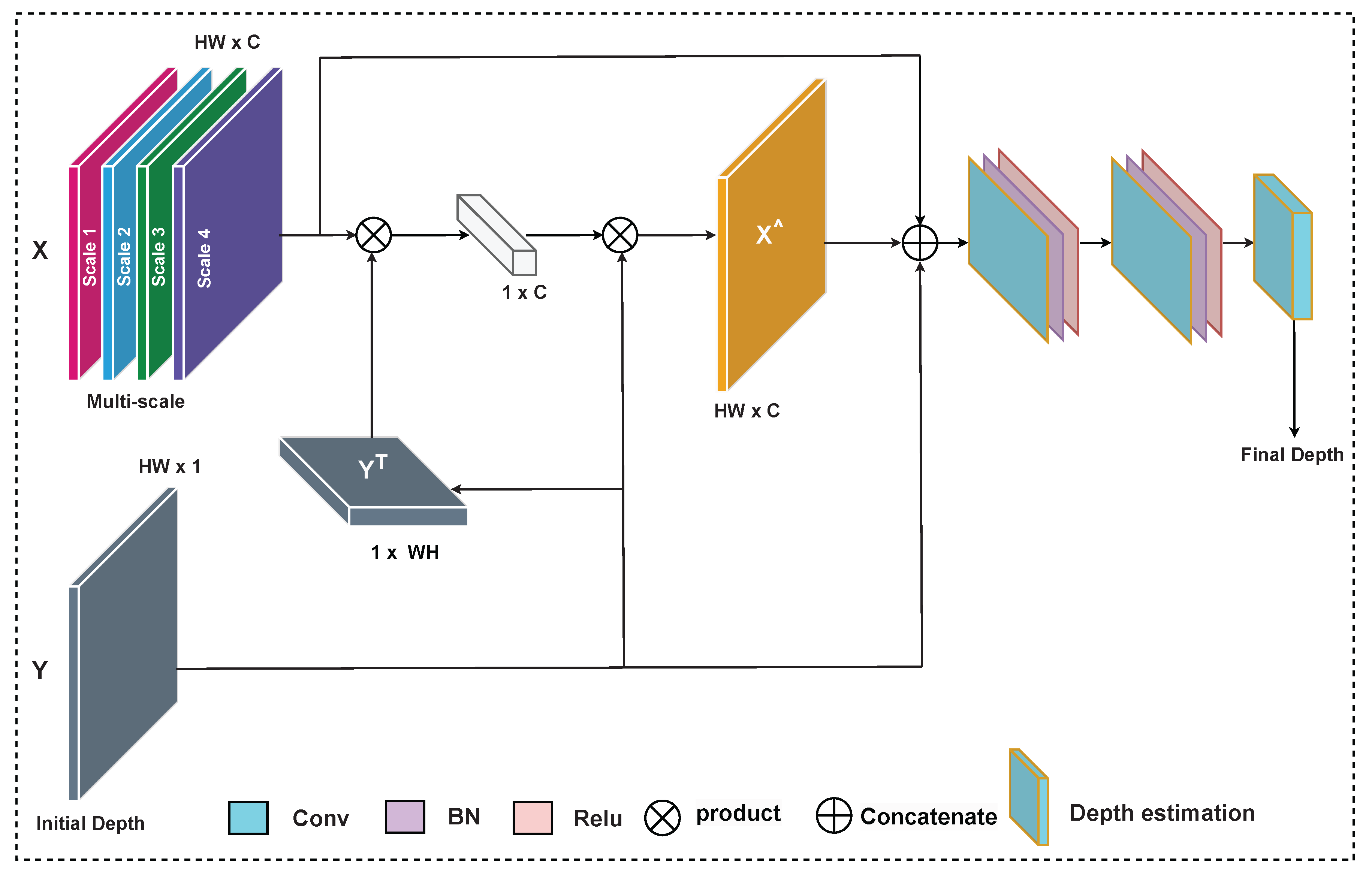
The Refining Attention Network (RAN) enhances the depth map by focusing on critical regions. This results in improved predictions, especially where objects have similar intensities or textures compared to their backgrounds. As shown in Figure 3,the RAN takes the refined multi-scale features X (the MSFA output) along with the coarse depth estimate Y from the decoder.
We explicitly compute the pairwise similarity between the coarse depth probability vectors (obtained by normalizing Y over spatial locations to form a soft distribution) and the multi-scale feature vectors at each spatial location. Specifically, we use a cosine similarity formulation:
Sim ( i , j ) = ( M i , j · P i , j ) M i , j P i , j
where M i , j is the feature vector from the aggregated MSFA output at pixel ( i , j ) and P i , j is the coarse depth probability vector. This similarity guides the weighting of attention within the RAN module.
The RAN module processes these similarity-enhanced features through two successive 5 × 5 convolutions, each producing 64 channels, with batch normalization and ReLU followed by a final 3 × 3 convolution that reduces the output to a single-channel depth prediction. The result is a refined absolute depth map that preserves object discontinuities and fine-scale details.
This design is motivated by the limitations of traditional depth estimation methods, which often smooth out depth boundaries due to their loss functions and architectural constraints. Such smoothing leads to blurred object edges and missed fine structural details. The RAN module addresses this by applying a boundary-aware attention mechanism that adaptively emphasizes regions with strong depth discontinuities, such as object edges. By leveraging the similarity between coarse depth estimates and multi-scale features, the RAN module enhances edge precision and preserves important structural cues that are typically lost in conventional approaches.

3.3. Loss Functions

3.3.1. Multi-Scale Loss Function

To improve depth prediction accuracy across varying object sizes and scene structures, we incorporate a multi-scale loss function during training. Multi-scale loss functions are particularly effective in tasks where understanding both coarse layout and fine details is essential, such as image segmentation [39,40] and depth estimation [41,42]. They allow the model to learn from feature representations at different resolutions, encouraging more robust predictions at multiple levels of granularity.
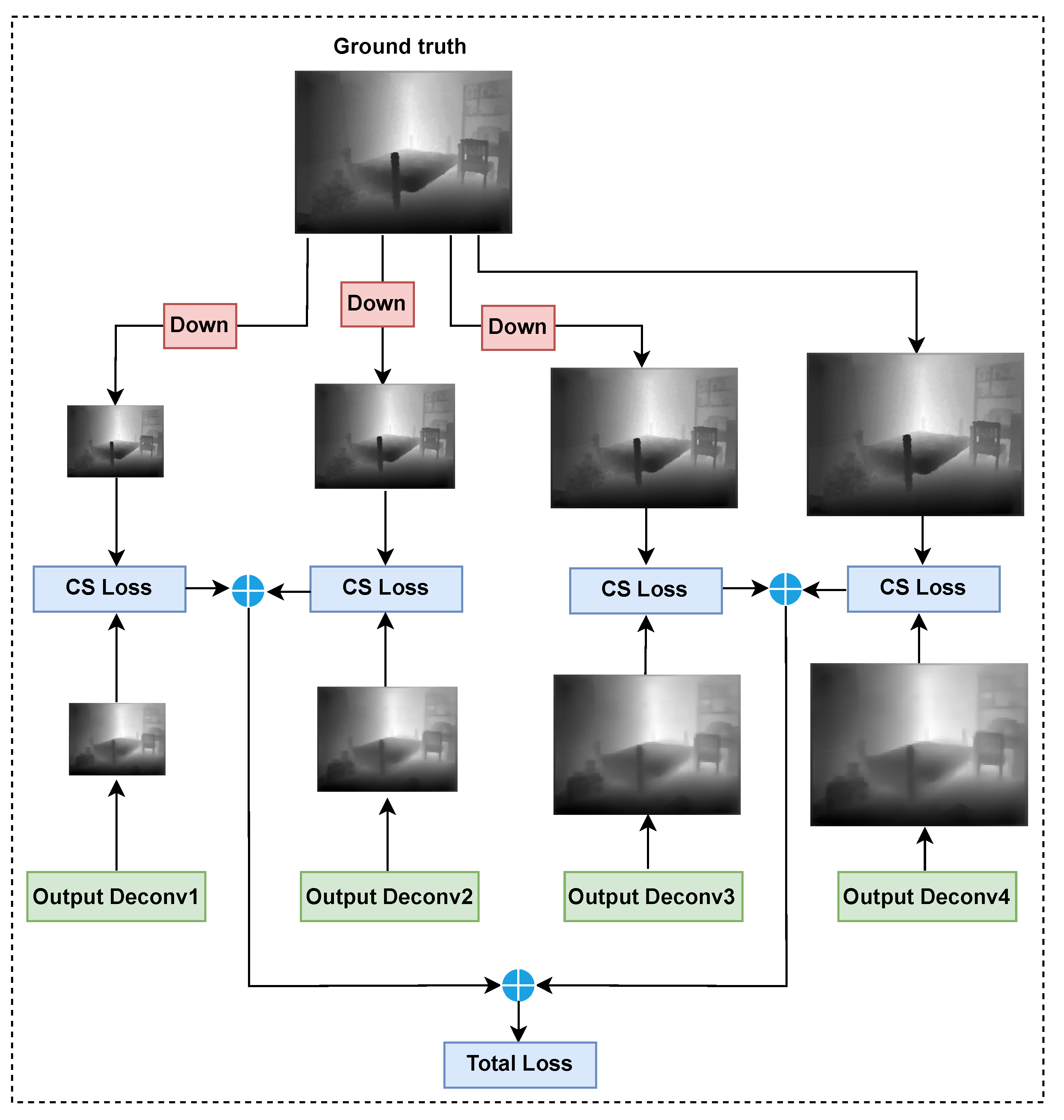
As illustrated in Figure 4, our framework employs a multi-scale loss architecture where the decoder network D generates intermediate depth estimates at multiple stages, each corresponding to a different resolution. To supervise these intermediate outputs, we downsample the ground truth depth map to match each decoder output scale. We then compute the Curvilinear Saliency (CS) loss [29,43] at each level. The CS loss focuses on capturing structural and edge-aware details, especially around object boundaries, which are often critical for depth perception.
Formally, the total multi-scale loss is computed as
M L = i = 1 N C S ( S i , Y i ) ,
where N is the number of scales (we use four), S i are the predicted depth maps from each decoder block, and Y i are the corresponding ground truth depth maps after downsampling.
This supervision strategy enables the network to learn depth features at different scales and ensures that both global context and local boundary information are preserved in the final depth prediction.
It is important to note that the proposed MSFA module operates on feature maps extracted from multiple decoder layers, not on rescaled versions of the input image. These decoder layers inherently produce features at different spatial resolutions and receptive field sizes due to the encoder–decoder architecture. Each layer captures depth cues from different perspectives, ranging from fine-grained local details to broader global structure. By aggregating these hierarchical feature maps, the MSFA module is able to better handle the scale variation present in real-world scenes. This multi-resolution fusion approach enhances the model’s ability to represent depth for objects at various distances and sizes in a way that cannot be achieved through simple uniform resizing of the input image.
This integration of multi-scale supervision through the CS loss combined with hierarchical multi-scale feature aggregation via the MSFA module jointly improves both learning stability and final depth prediction accuracy, particularly around object boundaries and in regions with complex depth transitions.

3.3.2. Content Loss Function

As proposed in [29], we formulate our monocular depth estimation problem as minimizing a reprojection error between the estimated depth Y ^ ( i , j ) (i.e., the refined depth map) and the ground truth Y ( i , j ) at training time, similar to [44]. Three loss functions are used to build our objective loss function.
The point-wise L 1 n o r m defined on the depth values is the first content loss L L 1 , which can be defined as follows:
L L 1 ( Y , Y ^ ) = 1 w h ( i = 1 w j = 1 h | Y ( i , j ) Y ^ ( i , j ) | )
where w and h are the width and height of the ground truth depth and i and j are the index of the pixel.
The Structural Similarity Index Measure (SSIM) loss index is used to evaluate the perceived quality of digital images. The SSIM loss function is a comprehensive reference metric used to evaluate the accuracy of depth images generated by the model compared to the corresponding ground truth. The SSIM index L S S I M can be defined as follows:
L S S I M ( Y , Y ^ ) = 1 2 ( 1 ( 2 μ Y ^ μ Y + c 1 ) ( 2 σ Y ^ Y + c 2 ) ( μ Y ^ 2 + μ Y 2 + c 1 ) ( σ Y ^ 2 + σ Y 2 + c 2 ) )
where μ Y ^ is the mean of Y ^ , σ Y ^ is the standard deviation of Y ^ , μ Y is the mean of Y, σ μ Y is the standard deviation of Y, σ Y ^ Y is the covariance of Y ^ , c 1 = 0 . 01 2 , and c 2 = 0 . 03 2 .
The Mean Square Error (MSE) is the third loss function ( L M S E ), which can be defined as
L M S E ( Y , Y ^ ) = 1 w h ( i = 1 w j = 1 h ( Y ( i , j ) Y ^ ( i , j ) ) 2 ) ,
L ( Y , Y ^ ) = α L L 1 ( Y , Y ^ ) + β L S S I M ( Y , Y ^ ) + γ L M S E ( Y , Y ^ ) ,
where α , β , and γ all equal 1.

3.3.3. Total Loss Function

The final objective function used to train the proposed model is L ( S i , Y i , Y , Y ^ ) , which is a combination of the two previously mentioned loss functions and can be defined as follows:
L ( S i , Y i , Y , Y ^ ) = α M L ( S i , Y i ) + β L ( Y , Y ^ )
where α and β are weighting factors empirically set to 0.6 and 0.4 , respectively, to achieve optimal performance across indoor and outdoor datasets. These weights control the balance between structural sharpness and global depth fidelity. A higher α emphasizes multi-scale structural refinement, improving edge clarity and small-object depth accuracy, while a higher β favors overall smoothness and pixel-wise consistency.
Although α = 0.6 and β = 0.4 are empirical settings, this weight combination was determined to have comprehensive optimality on both indoor and outdoor datasets through preliminary comparative experiments.

4. Experiments and Results

This section describes the experiments carried out to evaluate the model developed in this work. Both indoor and outdoor datasets were employed to assess the model, with data augmentation applied specifically to the outdoor dataset. Various evaluation metrics were employed to quantitatively measure the model’s performance in these experiments.

4.1. Dataset

We conducted all the experiments in this work on three publicly available datasets: the NYU Depth-v2 [45] and SUN RGB-D [46] datasets for indoor scenes, and the Make3D [47] dataset for outdoor scenes.

4.1.1. Indoor Scenes

  • NYU Depth-v2 dataset
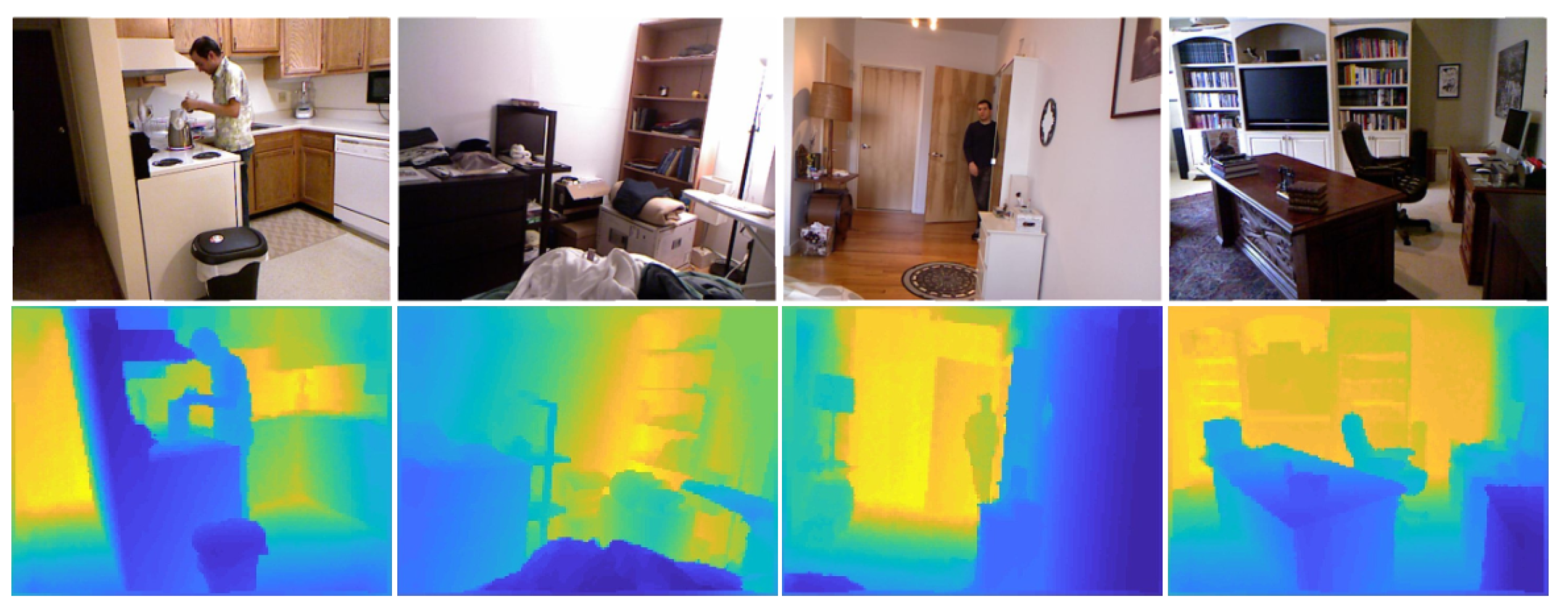
NYU Depth-v2 [45] is a public dataset that provides color images and depth maps for different indoor scenes captured at a resolution of 640 × 480 pixels [45]. The dataset contains raw frames captured by scanning various indoor scenes with a Microsoft Kinect, including 120K frames for training and 654 for testing. We trained our network models on a subset of Depth-v2 containing 50,000 images, as proposed in [44]. To feed the network, we resized all color images from 640 × 480 to 480 × 360 . The depth maps had an upper bound of 10 m. Figure 5 shows some examples from the NYU Depth-v2 dataset.
II.
SUN RGB-D dataset
SUN RGB-D is a public indoor scene dataset [46] with 10K training images and 5050 test images. The images are collected with four different sensors at a resolution of 730 × 530, providing high scene diversity. We did not perform training with this dataset, and only used it for evaluation. We cross-evaluated our pretrained model from the NYU dataset on the official test set of 5050 images without further fine-tuning. We resized all images from 730 × 530 to 480 × 360 as inputs to the network, and the depth maps had an upper bound of 10 m. Figure 6 shows some examples from the SUN RGB-D dataset.

4.1.2. Outdoor Scenes

  • Make3D dataset
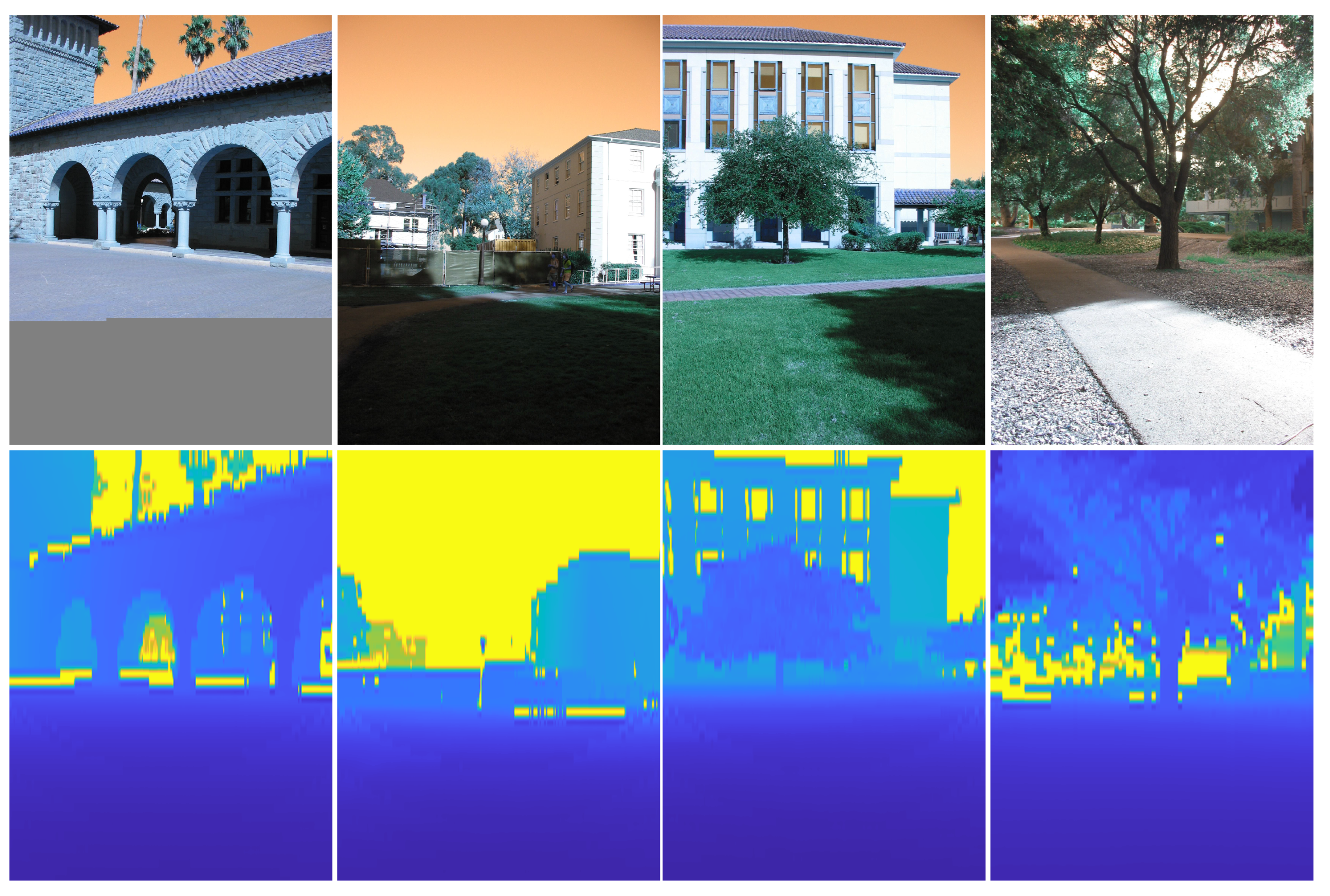
Make3D is a public outdoor dataset [47] with 400 training and 134 test images captured through a custom-built 3D scanner. The resolution of the ground-truth depth maps is limited to 305 × 55 pixels, whereas the original size of the RGB images is 2272 × 1704 pixels. To increase the number of training samples, we applied the data augmentation techniques described in the next subsection. We extended the original 400 training images to 11,000 images. Increasing the number of training images made the developed depth map estimation model more robust. Moreover, we resized all images to 460 × 345 prior to feeding them into the network. Figure 7 shows example images from the Make3D dataset.

4.2. Data Augmentation

To enhance the variety of training samples and improve the robustness of our model, we implemented several data augmentation strategies on the images in the Make3D dataset. These techniques were applied under diverse conditions, contributing to an expanded and more diverse training dataset. The employed data augmentation methods included:
  • Scaling: Random scaling in which each input image and its corresponding depth map underwent a random scale transformation with a factor S ∈ [0.5, 1.7].
  • Rotation: Random rotation involving adjustments of the input image and its corresponding depth map by angles R ∈ [−60, −45, −30, 30, 45, 60] degrees.
  • Gamma Correction: Variation in gamma correction for each input RGB image, with random adjustments G ∈ [1, 2.8].
  • Flipping: Random flipping, in which each input image and its corresponding depth map experienced horizontal flipping with a factor F ∈ [−1, 0, 1].
  • Translation: Random translation, entailing shifts of each input image and its corresponding depth map by T ∈ [−6, −4, −2, 2, 4, 6] pixels.
While these data augmentation techniques introduced slight distortions to the represented scenes, their application significantly enhanced the efficiency of the network compared to training the model without data augmentation.

4.3. Parameter Settings

Our approach was implemented using the PyTorch framework [48]. The proposed model underwent training for a total of 20 epochs, utilizing a batch size of 4. All experiments were conducted on a single GTX 1080TI GPU. We employed the Adam optimizer [49] with parameters of β 1 = 0.5 , β 2 = 0.999 and the initial learning rate set to 0.0001 . For the NYU Depth-v2 dataset, the learning rate was reduced by 10 % every three epochs, while for the Make3D dataset there was no reduction in the learning rate during training.
The encoder utilized pretrained ResNet-50 and SENet-154 layers. The computational time for each epoch during the training process was approximately 1 h and 50 min with a batch size of 4. For the Make3D dataset, the corresponding time was around 29 min per epoch with a batch size of 4. The online estimation of depth maps demonstrated performance of approximately 19.2 ms per image for both the NYU Depth-v2 and SUN RGB-D datasets. In contrast, the performance for the Make3D dataset was around 26 ms per image.

4.4. Evaluation Measures

This work aims to predict accurate dense depth images from monocular images. In this context, evaluating the results quantitatively is important for benchmarking performance and comparison with existing solutions; thus, the performance of the proposed model was evaluated under several different measures. The first measure is the threshold accuracy measure from [50], which is essentially an expectation that the depth value error of a given pixel in T will be lower than a threshold t h r Z , defined as
δ Z = E T [ F ( max ( B ( i ) B ^ ( i ) , B ^ ( i ) B ( i ) ) < t h r Z ) ] ,
where F ( · ) is an indicator function that returns either 0 or 1. We set t h r = 1.25 and Z { 1 , 2 , 3 } , similar to [50].
The second measure is the Root Mean Square Error (RMSE), which provides a quantitative measure of per-pixel error, computed as follows (13):
R M S E = 1 n i T ( B p r e d , ( i ) B g t , ( i ) ) 2
where B g t , ( i ) is the real depth of pixel i, B p r e d , ( i ) is the associated predicted depth, T is the set of valid pixels (i.e., both the ground truth and predicted depth pixels that do not have depth values equal to zero or non-black regions), and n is the cardinality of T.
The third measure is the average relative error ( r e l ), which is defined as the ratio of the absolute error of the measurement to the actual measurement and determines the magnitude of the absolute error in terms of the actual size of the measurement. The r e l is computed as follows (14):
r e l = 1 w h x = 1 w y = 1 h | B ( x , y ) B ^ ( x , y ) | B ( x , y ) .
The fourth measure is the base-10 log ( l o g 10 ), also known as the common logarithm or decadic logarithm, computed as follows (15):
l o g 10 = 1 w h x = 1 w y = 1 h | l o g 10 B ( x , y ) l o g 10 B ^ ( x , y ) | .

4.5. Results and Discussion

4.5.1. Ablation Study

First, we performed an ablation study to assess the impact of different stages of the proposed autoencoder. The following configurations were considered:
  • Baseline (BL): Basic autoencoder with four content loss functions: point-wise ( L 1 ) loss, mean squared error ( L m s e ) loss, the logarithm of depth errors ( L d e p t h ) loss, and structural similarity index measure ( L s s i m ) loss.
  • BLSC: BL model with skip connections from the encoder layers to the corresponding decoder layers.
  • BLSC + MSFA: BLSC model with Multi-Scale Feature Aggregation Network (MSFA).
  • BLSC + RAN: BLSC model with Refining Attention Network (RAN).
  • BLSC + ML: BLSC model with multi-loss function.
  • BLSC + ML + MSFA + RAN: BLSC model with multi-loss function, MSFA, and RAN.
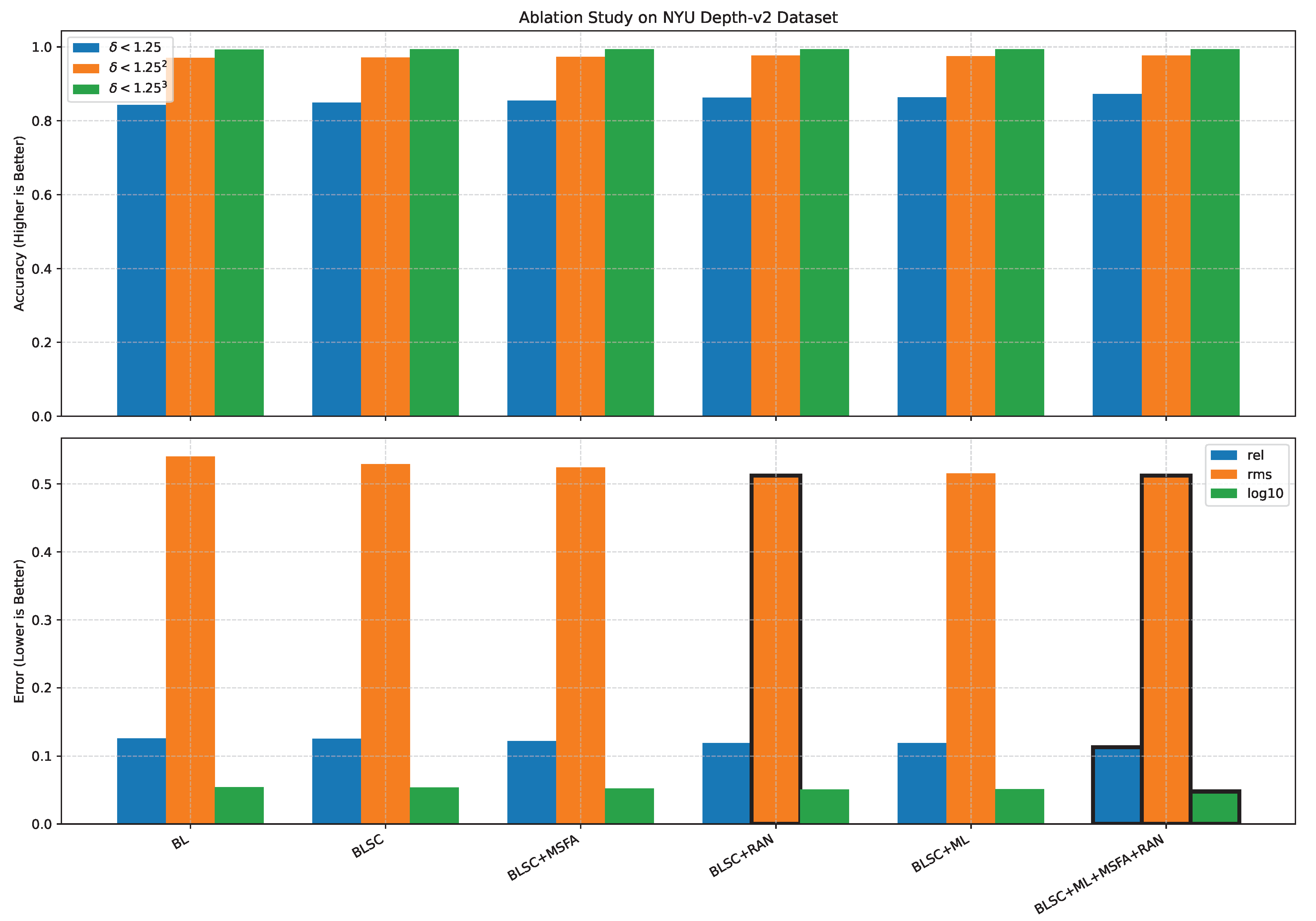
Table 1 shows the quantitative results of the ablation study for the NYU Depth-v2 dataset. The performance of the proposed model (BLSC + ML + MSFA + RAN) yielded the best results among other variations of the proposed model in terms of δ Z ( t h r = 1.25 ) as well as r m s , r e l , and l o g 10 errors. The accuracy of δ Z ( t h r = 1.25 ) improved by around 3 % compared to the baseline model (BL). Similarly, for the r e l error, the proposed model yielded a significant improvement of 0.013 % compared to the BL model. Adding the MSFA module to the baseline model improved accuracy by 1.24 % and reduced the r e l error by 0.0041 % . Adding the RAN module to the baseline model improved accuracy by 2.04 % and reduced the r e l error by 0.0067 % . Applying the multi-scale loss also yielded a significant accuracy improvement and a considerable reduction in the r e l error compared to the BL model, with differences of 2.11 % and 0.0071 % , respectively. Figure 8 presents the ablation study results on the NYU Depth-v2 dataset, demonstrating the systematic contribution of each architectural component. The baseline model (BL) establishes the initial performance, achieving accuracy values above 0.8 for all δ thresholds. The addition of skip connections (BLSC) provides modest improvements across all metrics. Incorporating Multi-Scale Aggregation (BLSC + MSA) significantly enhances performance, particularly in the δ < 1.25 threshold accuracy and error reduction. The Multi-Scale Attention Network (BLSC + MAN) and Multi-Loss function (BLSC + ML) components each contribute additional improvements. The complete model (BLSC + ML + MSA + RAN) achieves the best performance across all metrics, with accuracy values exceeding 0.98 for all δ thresholds and the lowest error rates in rel, rms, and log 10 metrics. This systematic improvement validates the synergistic effect of all proposed components in achieving state-of-the-art depth estimation performance.
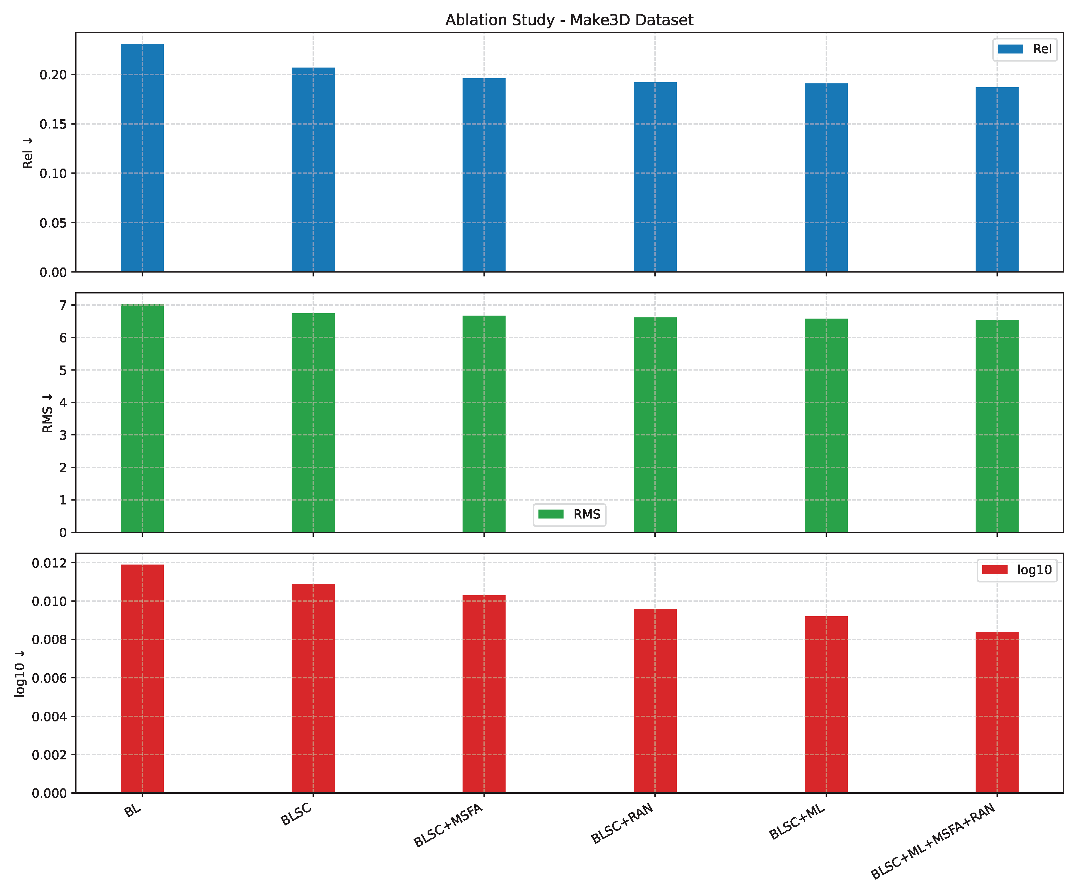
In Table 2, we present the quantitative outcomes from a similar ablation study conducted on the Make3D dataset. Among the various configurations we examined, the BLSC + ML + MSFA + RAN model exhibited the smallest errors, specifically in terms of the r m s , r e l , and l o g 10 error metrics. Figure 9 presents a comprehensive ablation study demonstrating the individual contributions of each component in our DAR-MDE architecture on the Make3D dataset. The baseline model (BL) establishes the initial performance benchmark. The systematic addition of components shows consistent improvements: skip connections (BLSC) provide initial enhancement, while the Multi-Scale Aggregation (BLSC + MSA) and Multi-scale Attention Network (BLSC + MAN) components contribute significantly to error reduction. The Multi-Loss function (BLSC + ML) further improves performance, and our complete model (ML + MSA + RAN) achieves the best results across all three metrics, validating the synergistic effect of all proposed components.

4.5.2. Performance Analysis

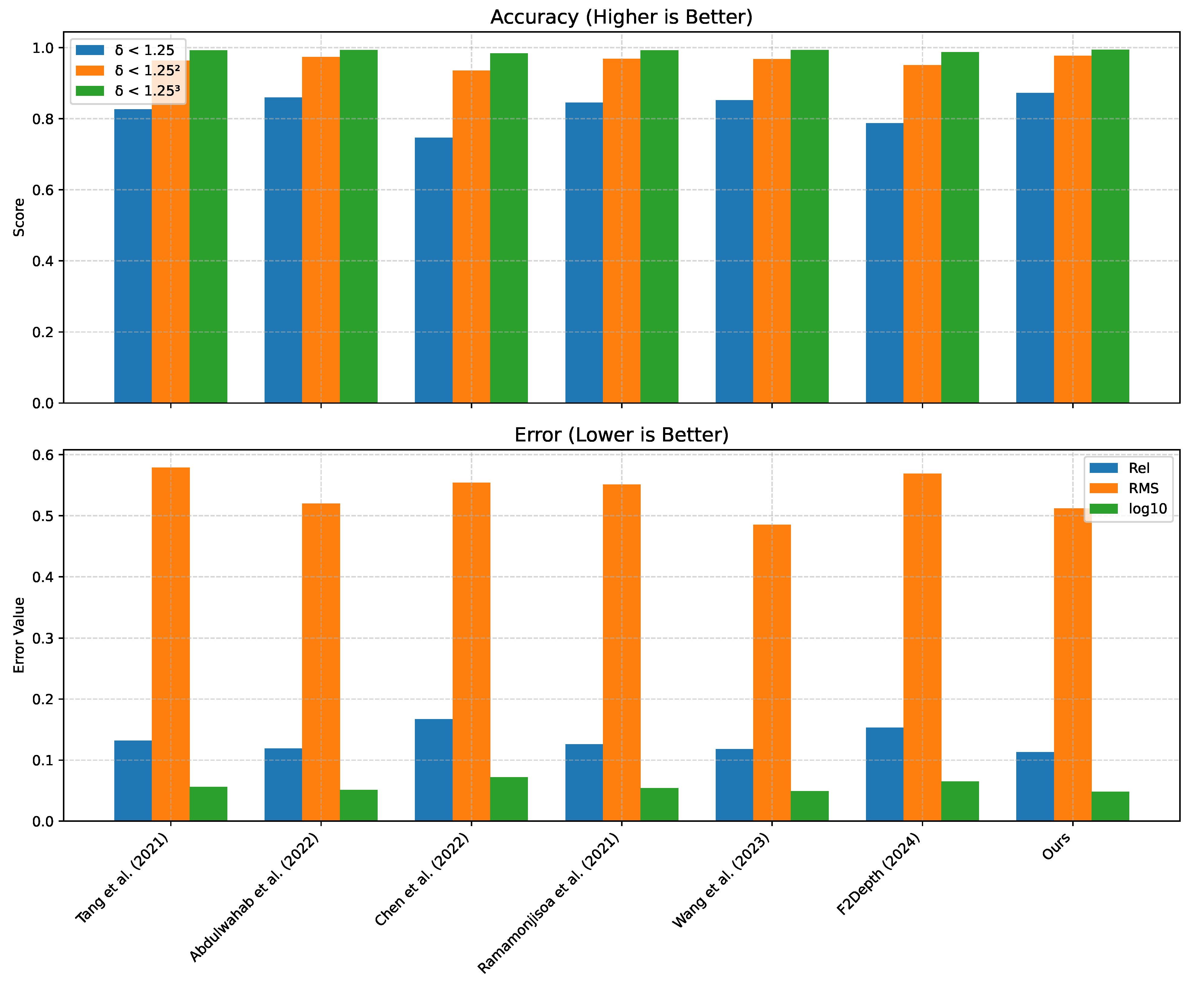
Next, we compared the proposed model against six alternative models [25,29,51,52,53,54]. In Table 3, we show evaluation measures on the NYU Depth-v2 dataset for the seven tested approaches. The accuracy of our proposed model was superior for δ Z ( thr = 1.25 ) , δ Z ( thr = 1 . 25 2 ) and the l o g 10 error. In addition, δ Z ( thr = 1.25 ) shows an improvement of 1.34 % and δ Z ( thr = 1 . 25 2 ) , an improvement of 0.33 % compared to [29], which is the best second method. Concerning δ Z ( thr = 1 . 25 3 ) , our model yielded an improvement of 0.08 % compared to the other six methods. The model proposed in [25] provided the lowest r m s error rate, but with a difference of only 0.027 compared to our proposed model. The recent method from [54] also lags behind our model, with lower accuracy in all δ Z thresholds and higher l o g 10 and r e l errors.
From testing on NYU Depth-v2, we can note that our model provided the best accuracy for δ Z ( thr = 1.25 ) , δ Z ( thr = 1 . 25 2 ) and δ Z ( thr = 1 . 25 3 ) , which is the most restrictive threshold. In addition, our model scored the lowest l o g 10 error of ( 0.048 ) and the lowest r e l error of ( 0.113 ). From testing on Make3D, we can note that our model scored the lowest l o g 10 error of ( 0.007 ) and the lowest r e l error of ( 0.008 ).
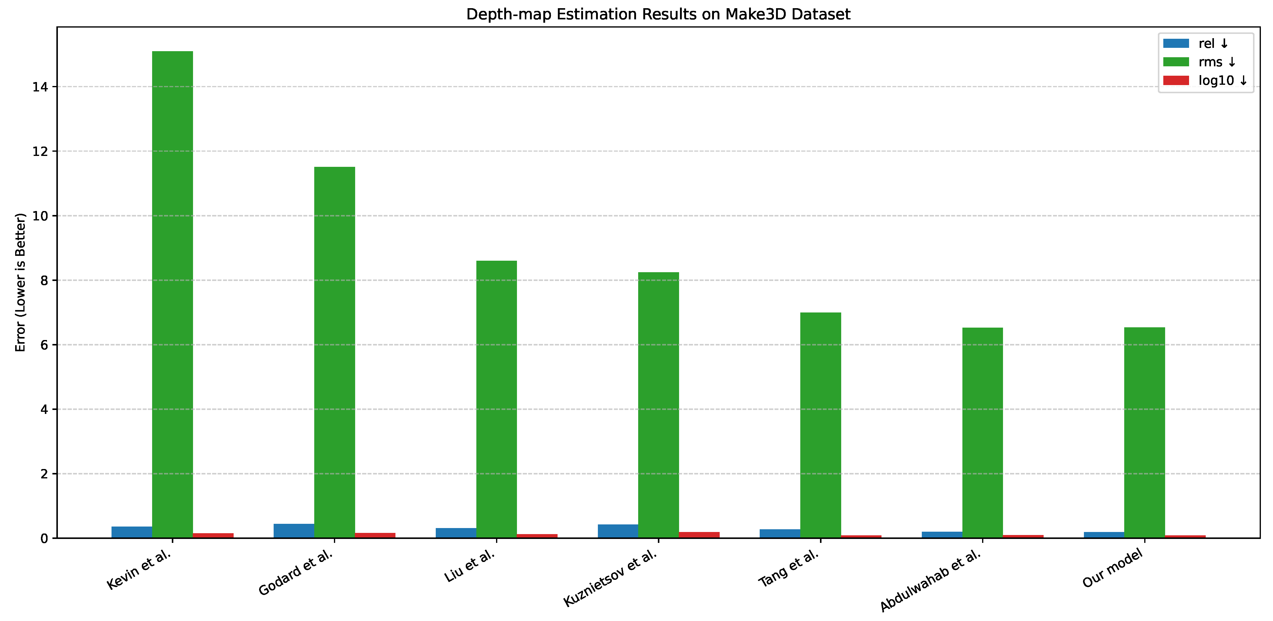
In Table 4, we evaluated our proposed DAR-MDE model against six state-of-the-art methods on the Make3D dataset [29,50,53,55,56,57]. Table 4 presents the evaluation results using three key error metrics: relative error (rel), root mean square error (rms), and log 10 error. Our proposed model demonstrates superior performance across most evaluation criteria.
The DAR-MDE model achieves the best relative error of 0.187 , representing a significant improvement of 4.1 % compared to the second-best method by Abdulwahab et al. [29] ( 0.195 ). For the log 10 error metric, our model attains the lowest error of 0.084 , showing a notable improvement of 7.7 % over the second-best performing method. Regarding the rms error, while Abdulwahab et al. [29] achieves the lowest value of 6.522 , our model follows closely with 6.531 , showing only a marginal difference of 0.009 .
The substantial improvements in relative error and log 10 error demonstrate the effectiveness of our Multi-Scale Feature Aggregation (MSFA) and Refining Attention Network (RAN) components in capturing fine-grained depth details and preserving object boundaries. The competitive rms performance further validates the robustness of our approach. Notably, our model significantly outperforms earlier methods such as Karsch et al. [55] and Godard et al. [56], showing improvements of over 48 % and 58 % in relative error, respectively. These results confirm that our DAR-MDE model achieves state-of-the-art performance on the challenging Make3D dataset, particularly excelling in relative depth accuracy and logarithmic error minimization.
In addition, Figure 10 and Figure 11 provide examples of depth estimates from the NYU Depth-v2 and Make3D testing sets, comparing our model’s accuracy and error rates to those of state-of-the-art models. The results show that our proposed model outperforms the other tested methods.
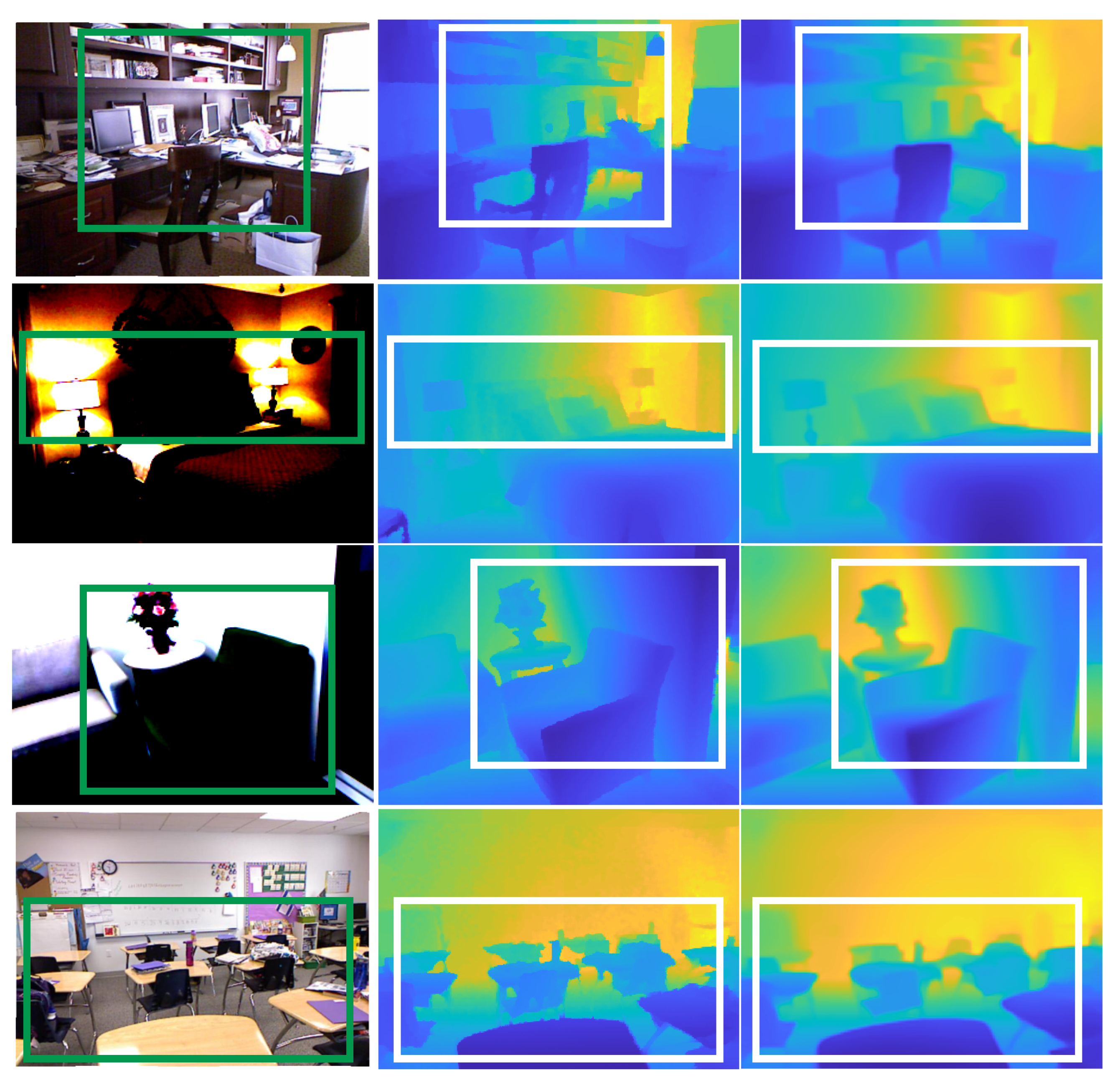
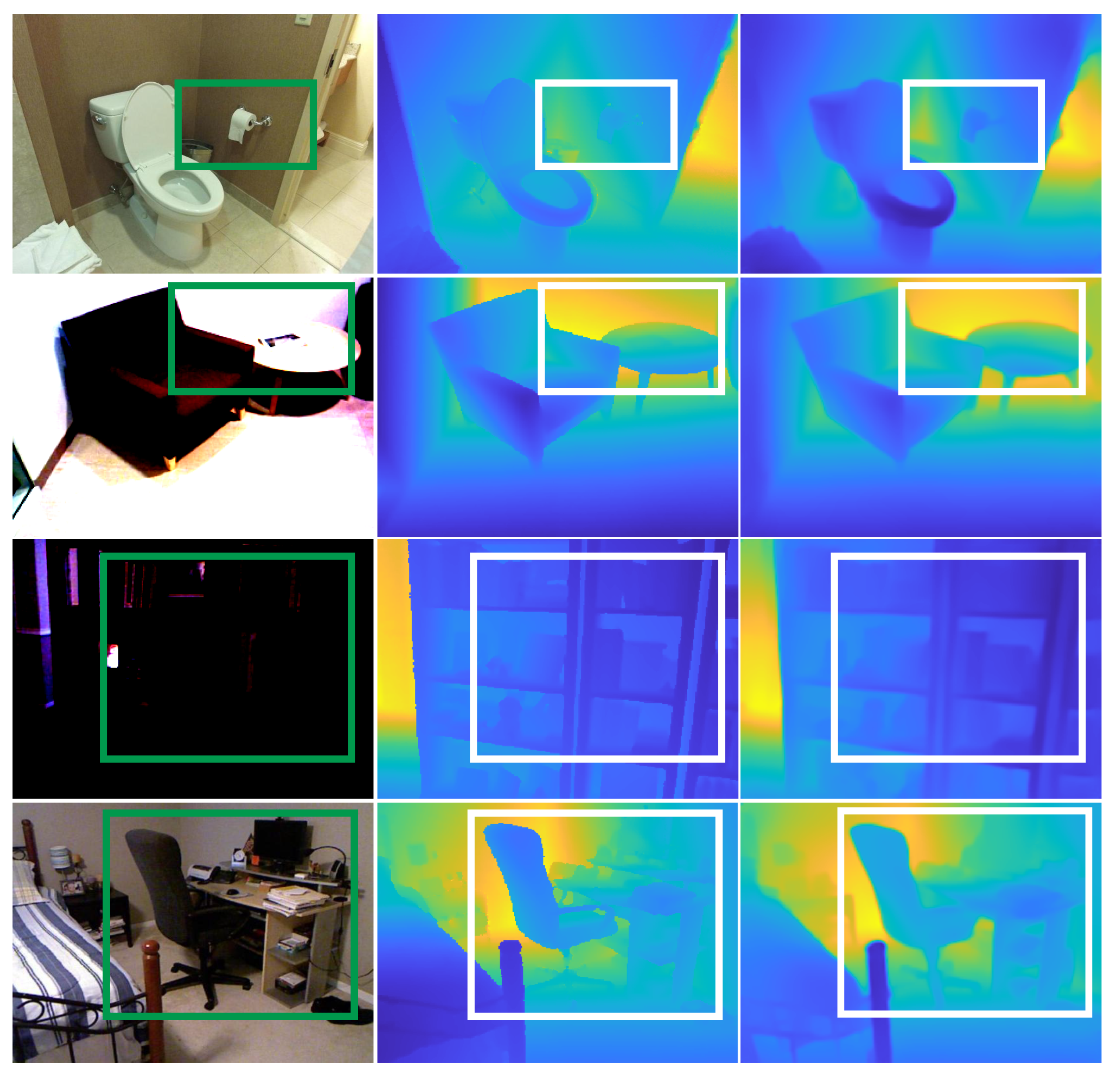
To evaluate the performance of our proposed model, we selected random images from the NYU Depth-v2 test set to show the model’s ability to produce accurate depth maps (refer to Figure 12). It is worth noting that the model can generate depth maps under various conditions. The model learned to identify the correct objects within the images. The model could generally estimate correct depth values for small objects in the scene (refer to Figure 12, Row 1) and objects affected by lighting (refer to Figure 12, Row 2). It was also able to accurately detect objects in dark areas (refer to Figure 12, Row 3) even in geometrically complex areas (refer to Figure 12, Row 4).
Table 3. Results for depth map estimation from color images with the NYU Depth v2 dataset for different measures and state-of-the-art methods. The last row shows the results obtained by our proposed model. Arrows indicate performance direction: ↑ (higher is better), ↓ (lower is better).
MethodAccuracy: Higher Is BetterError: Lower Is Better
δ < 1 . 25 δ < 1 . 25 2 δ < 1 . 25 3 rel ↓rms ↓log10 ↓
Tang et al. [53]0.8260.9630.9920.1320.5790.056
Abdulwahab et al. [29]0.85910.97330.99320.1190.5200.051
Chen et al. [51]0.7460.9350.9840.1670.5540.072
Ramamonjisoa et al. [52]0.84510.96810.99170.12580.5510.054
WangandPiao et al. [25]0.8520.9670.9930.1180.4850.049
Guo et al. [54]0.7870.9500.9870.1530.5690.065
Our model (DAR-MDE)0.87250.97660.9940.1130.5120.048
Bold values indicate the best performance achieved by the complete model.
Figure 10. Results in terms of accuracy and the three error measures for the six tested state-of-the-art models [25,29,51,52,53,54] and our proposed model on the NYU Depth-v2 dataset. The top panel shows accuracy metrics ( δ < 1.25 , δ < 1 . 25 2 , δ < 1 . 25 3 , higher is better), while the bottom panel shows error metrics (rel: relative error, rms: root mean square error, log 10 : logarithmic error, lower is better).
Jsan 14 00090 g010
Table 4. Results for depth map estimation from color images with the Make3D dataset for different measures and state-of-the-art methods. The last row shows the results obtained by our proposed model. Arrows (↓) indicate that lower values are better for all error metrics.
Methodrel ↓rms ↓log10 ↓
Kevin et al. [55]0.36115.10.148
Godard et al. [56]0.44311.5130.156
Liu et al. [50]0.3148.600.119
Kuznietsov et al. [57]0.4218.240.190
Tang et al. [53]0.2766.990.086
Abdulwahab et al. [29]0.1956.5220.091
Our model (DAR-MDE)0.1876.5310.084
Bold values indicate the best performance achieved by the complete model.
Figure 11. Results in terms of the three error measures for the six tested state-of-the-art models [29,50,53,55,56,57] and our proposed model on the Make3D dataset. Arrows (↓) indicate that lower values represent better performance for all error metrics (rel: relative error, rms: root mean square error, log 10 : logarithmic error).
Jsan 14 00090 g011
Figure 12. Input images (Column 1), ground-truth depth maps (Column 2), and estimated depth maps (Column 3) with the NYU Depth-v2 dataset. Green boxes highlight challenging regions in the input images: small objects like monitors and equipment (Row 1), areas affected by strong lighting conditions (Row 2), objects in dark/low-light areas (Row 3), and geometrically complex scenes with multiple depth layers (Row 4). White boxes in the depth maps correspond to the same regions, enabling direct comparison between ground-truth and estimated depth predictions.
Jsan 14 00090 g012
In Figure 12, DAR-MDE shows superior resilience in scenes with strong illumination contrast and partial occlusion. Unlike baseline methods, our model maintains consistent depth estimation across shadowed and saturated areas, preserving object shapes and avoiding flattening effects. This is primarily due to the multi-scale contextual reasoning provided by MSFA and the contour-sensitive refinement enabled by RAN. In low-light regions or areas with blurred textures, the attention mechanism still guides the network to infer plausible depth transitions based on nearby structure and semantics. Occlusion boundaries, where abrupt depth discontinuities typically confuse local filters, are also handled better by DAR-MDE, as reflected by the cleaner edge transitions visible in the predictions. These observations indicate that our model generalizes well across diverse environmental conditions, confirming its robustness not only on a metric level but also in terms of visual fidelity and scene understanding.
To assess the generalization ability of our proposed model, we evaluated it on the SUN RGB-D dataset without fine-tuning, using models trained solely on the NYU Depth v2 dataset. Table 5 reports the quantitative comparison against a wide range of state-of-the-art approaches from 2019 to 2025. Our model achieved the best performance across most evaluation metrics. Specifically, using the SENet-154 encoder, our model reached the highest accuracy under the strict δ < 1.25 threshold with a score of 0.865, and also achieved the lowest errors in terms of rel (0.120), rms (0.405), and log 10 (0.054). The ResNet-50 variant of our model also demonstrated strong performance, surpassing most existing methods in both accuracy and error metrics.
Compared to recent transformer-based methods, such as those using the Swin-Large and SwinV2-Large backbones, our approach remains highly competitive. While SwinV2-Large [58] achieved a slightly higher δ < 1.25 score of 0.861 and the lowest rms error of 0.355, our model consistently outperformed it in terms of overall accuracy–error balance, especially when the full metric sets are considered. Notably, our SENet-154 model achieved a higher δ < 1.25 than all listed methods, including recent models from 2023 to 2025, while maintaining lower or comparable error values. In Figure 13, we presents a comprehensive comparison of our DAR-MDE model against the state-of-the-art methods on the SUN RGB-D dataset. The results demonstrate that our model achieves competitive performance across all evaluation metrics, particularly excelling in accuracy measures while maintaining low error rates.
These results highlight the robustness and effectiveness of our model across diverse architectural baselines. Its strong performance, particularly under the strict δ < 1.25 threshold and key error metrics, demonstrates its capacity to produce precise and reliable depth estimates even when evaluated on unseen datasets.
To further evaluate the performance of the proposed model, we selected random images from the SUN RGB-D test set to show the model’s ability to produce accurate depth maps (refer to Figure 14). It is worth noting that the model can generate depth maps under various conditions. The model learned to identify the correct objects within the images. The model could generally estimate correct depth values for small objects in the scene (refer to Figure 14, Row 1) and objects affected by lighting (refer to Figure 14, Row 2). It was also able to accurately detect objects in dark areas (refer to Figure 14, Row 3) even in geometrically complex areas (refer to Figure 14, Row 4).
Table 5. Results for depth map estimation using color images from the NYU Depth v2 dataset for training and images from the SUN RGB-D dataset for testing. The last rows show results obtained with recent state-of-the-art methods (2023–2025) and our proposed model using ResNet-50 and SENet-154 networks. Note: – indicates that the respective metric was not reported in the original paper. Arrows indicate performance direction: ↑ (higher is better), ↓ (lower is better).
MethodEncoderAccuracy: Higher Is BetterError: Lower Is Better
δ < 1 . 25 δ < 1 . 25 2 δ < 1 . 25 3 rel ↓rms ↓log10 ↓
Chen et al. [59]SENet-1540.7570.9430.9840.1660.4940.071
Yin et al. [60]ResNeXt-1010.6960.9120.9730.1830.5410.082
Lee et al. [20]DenseNet-1610.7400.9330.9800.1720.5150.075
Bhat et al. [61]E-B5 + Mini-ViT0.7710.9440.9830.1590.4760.068
Li et al. [62]ResNet-180.7380.9350.9820.1750.5040.074
Li et al. [62]Swin-Tiny0.7600.9450.9850.1620.4780.069
Li et al. [62]Swin-Large0.8050.9630.9900.1430.4210.061
Zhao et al. [58]SwinV2-Large0.8610.1210.355
Li et al. [62]Swin-Large0.8050.9630.990.1430.4210.061
Hu et al. [63]SwinV2-Large0.8070.9670.9920.1390.4210.061
Our Model (DAR-MDE)ResNet-500.8600.9570.9770.1240.4100.057
Our Model (DAR-MDE)SENet-1540.8650.9600.9800.1200.4050.054
Bold values indicate the best performance achieved by the complete model.

5. Conclusions

This paper has presented a deep learning approach that uses an autoencoder network with a Multi-Scale Feature Aggregation and a Refining Attention Network to refine the final estimated depth map and preserve global depth information in the combined depth scales. The proposed model uses a multi-scale loss function, which uses different depth scales from each block in the decoder part to accurately compare the ground truth to the generated depth map and force the autoencoder to generate a correct dense depth image. The Curvilinear Saliency loss is used for multi-scale loss to preserve the object boundaries in the estimated depth map. Combining the depth scale outputs through the Multi-Scale Feature Aggregation network improves the model’s overall performance in estimating object depth information regardless of scale and viewpoint. Afterwards, the estimated depth is refined using a Refining Attention Network, which contains an attention module to improve the model’s diversity and generate more accurate predictions.
The proposed method achieves comparable depth estimation based on monocular vision to existing methods on both the NYU Depth v2 and SUN RGB-D datasets. The depth maps generated by our model show accurate dense depth, which is helpful for semantic mapping and visual odometry. While we did not explicitly benchmark scenarios such as reflective surfaces or low-texture regions, the architectural components—particularly MSFA and RAN—help to mitigate such challenges by enabling the network to focus on contextual depth cues and boundary-aware refinement.
We also note that the choice of the loss weights α and β in our final objective function allows for balancing between multi-scale structural preservation and pixel-wise content accuracy; future work will explore adaptive strategies for these parameters in order to further enhance robustness.
Additionally, our approach occasionally faces challenges under extreme reflectivity or heavy occlusion scenarios, which are common in monocular depth estimation. As part of future work, we aim to integrate uncertainty-aware modules or hybrid RGB–depth priors to alleviate these limitations and extend the applicability of our approach to more complex environments.
Furthermore, the proposed approach is tailored for RGB-only input and does not rely on additional modalities such as LiDAR or infrared, meaning that it can offer a lightweight and deployable solution for applications where multimodal data are unavailable. Part of our ongoing work is to develop an algorithm that combines camera parameters with generated depth images to calculate an accurate absolute distance applicable to autonomous vehicles in order to help them safely navigate their environments.

Author Contributions

Conceptualization and Methodology, S.A. and H.A.R.; Validation, M.T.E.-M.; Resources, D.P.; Writing—original draft, S.A. and M.T.E.-M.; Writing—review & editing, H.A.R. and D.P.; Supervision, H.A.R. and D.P. All authors have read and agreed to the published version of the manuscript.

Funding

Financial support was provided by a pre-Doctoral grant (FI 2020) from the Catalan government.

Conflicts of Interest

The authors declare no conflicts of interest.

Abbreviations

The following abbreviations are used in this manuscript:
MDEMonocular Depth Estimation
CNNConvolutional Neural Network
MSFAMulti-Scale Feature Aggregation
RANRefining Attention Network
DAR-MDEDual-Attention Refining Monocular Depth Estimation
NYU Depth v2New York University Depth Dataset v2
SUN RGB-DSUN RGB-D Dataset
MSEMean Squared Error
RMSERoot Mean Square Error
SSIMStructural Similarity Index Measure
relAverage Relative Error
MSMulti-Scale
GTGround Truth
GPUGraphics Processing Unit
LiDARLight Detection and Ranging
ADAMAdaptive Moment Estimation
GANGenerative Adversarial Network
SOTAState-of-the-Art

References

  1. Chiu, C.H.; Astuti, L.; Lin, Y.C.; Hung, M.K. Dual-Attention Mechanism for Monocular Depth Estimation. In Proceedings of the 2024 16th International Conference on Computer and Automation Engineering (ICCAE), Melbourne, Australia, 14–16 March 2024; IEEE: Piscataway, NJ, USA, 2024; pp. 456–460. [Google Scholar]
  2. Yang, Y.; Wang, X.; Li, D.; Tian, L.; Sirasao, A.; Yang, X. Towards Scale-Aware Full Surround Monodepth with Transformers. arXiv 2024, arXiv:2407.10406. [Google Scholar] [CrossRef]
  3. Tang, S.; Lu, T.; Liu, X.; Zhou, H.; Zhang, Y. CATNet: Convolutional attention and transformer for monocular depth estimation. Pattern Recognit. 2024, 145, 109982. [Google Scholar] [CrossRef]
  4. Liu, J.; Cao, Z.; Liu, X.; Wang, S.; Yu, J. Self-supervised monocular depth estimation with geometric prior and pixel-level sensitivity. IEEE Trans. Intell. Veh. 2022, 8, 2244–2256. [Google Scholar] [CrossRef]
  5. Hu, D.; Peng, L.; Chu, T.; Zhang, X.; Mao, Y.; Bondell, H.; Gong, M. Uncertainty Quantification in Depth Estimation via Constrained Ordinal Regression. In Proceedings of the European Conference on Computer Vision (ECCV), Tel Aviv, Israel, 23–27 October 2022; Available online: https://www.ecva.net/papers/eccv_2022/papers_ECCV/papers/136620229.pdf (accessed on 14 August 2025).
  6. Wang, Y.; Piao, X. Scale-Aware Deep Networks for Monocular Depth Estimation. In Proceedings of the CVPR, Seattle, WA, USA, 16–22 June 2024. [Google Scholar]
  7. Wang, W.; Yin, B.; Li, L.; Li, L.; Liu, H. A Low Light Image Enhancement Method Based on Dehazing Physical Model. Comput. Model. Eng. Sci. (CMES) 2025, 143, 1595–1616. [Google Scholar] [CrossRef]
  8. Zhang, Z. Lightweight Deep Networks for Real-Time Monocular Depth Estimation. In Proceedings of the ICRA, London, UK, 29 May–2 June 2023. [Google Scholar]
  9. Yoon, S.; Lee, J. Context-Aware Depth Estimation via Multi-Modal Fusion. In Proceedings of the CVPR, Seattle, WA, USA, 16–22 June 2024. [Google Scholar]
  10. Shakibania, H.; Raoufi, S.; Khotanlou, H. CDAN: Convolutional dense attention-guided network for low-light image enhancement. Digit. Signal Process. 2025, 156, 104802. [Google Scholar] [CrossRef]
  11. Ding, L. Attention-Guided Depth Completion from Sparse Data. In Proceedings of the European Conference on Computer Vision (ECCV), Milan, Italy, 29 September–4 October 2024. [Google Scholar]
  12. Chen, Y.; Zhao, H.; Hu, Z.; Peng, J. Attention-based context aggregation network for monocular depth estimation. Int. J. Mach. Learn. Cybern. 2021, 12, 1583–1596. [Google Scholar] [CrossRef]
  13. Eigen, D.; Puhrsch, C.; Fergus, R. Depth map prediction from a single image using a multi-scale deep network. Adv. Neural Inf. Process. Syst. 2014, 2, 2366–2374. [Google Scholar]
  14. Xu, D.; Ricci, E.; Ouyang, W.; Wang, X.; Sebe, N. Multi-scale continuous CRFs as sequential deep networks for monocular depth estimation. In Proceedings of the IEEE Conference on Computer Vision and Pattern Recognition, Honolulu, HI, USA, 21–26 July 2017; pp. 5354–5362. [Google Scholar]
  15. Liu, C.; Gu, J.; Kim, K.; Narasimhan, S.G.; Kautz, J. Neural RGB(r)D sensing: Depth and uncertainty from a video camera. In Proceedings of the IEEE/CVF Conference on Computer Vision and Pattern Recognition, Long Beach, CA, USA, 15–20 June 2019; pp. 10986–10995. [Google Scholar]
  16. Masoumian, A.; Rashwan, H.A.; Cristiano, J.; Asif, M.S.; Puig, D. Monocular depth estimation using deep learning: A review. Sensors 2022, 22, 5353. [Google Scholar] [CrossRef]
  17. Simsar, E.; Örnek, E.P.; Manhardt, F.; Dhamo, H.; Navab, N.; Tombari, F. Object-Aware Monocular Depth Prediction with Instance Convolutions. IEEE Robot. Autom. Lett. 2022, 7, 5389–5396. [Google Scholar] [CrossRef]
  18. Ji, W.; Yan, G.; Li, J.; Piao, Y.; Yao, S.; Zhang, M.; Cheng, L.; Lu, H. DMRA: Depth-induced multi-scale recurrent attention network for RGB-D saliency detection. IEEE Trans. Image Process. 2022, 31, 2321–2336. [Google Scholar] [CrossRef]
  19. Aich, S.; Vianney, J.M.U.; Islam, M.A.; Liu, M.K.B. Bidirectional attention network for monocular depth estimation. In Proceedings of the 2021 IEEE International Conference on Robotics and Automation (ICRA), Xi’an, China, 30 May–5 June 2021; IEEE: Piscataway, NJ, USA, 2021; pp. 11746–11752. [Google Scholar]
  20. Lee, J.H.; Han, M.K.; Ko, D.W.; Suh, I.H. From big to small: Multi-scale local planar guidance for monocular depth estimation. arXiv 2019, arXiv:1907.10326. [Google Scholar]
  21. Jung, H.; Kim, Y.; Min, D.; Oh, C.; Sohn, K. Depth prediction from a single image with conditional adversarial networks. In Proceedings of the 2017 IEEE International Conference on Image Processing (ICIP), Beijing, China, 17–20 September 2017; IEEE: Piscataway, NJ, USA, 2017; pp. 1717–1721. [Google Scholar]
  22. Wofk, D.; Ma, F.; Yang, T.J.; Karaman, S.; Sze, V. Fastdepth: Fast monocular depth estimation on embedded systems. In Proceedings of the 2019 International Conference on Robotics and Automation (ICRA), Montreal, QC, Canada, 20–24 May 2019; IEEE: Piscataway, NJ, USA, 2019; pp. 6101–6108. [Google Scholar]
  23. Moukari, M.; Picard, S.; Simon, L.; Jurie, F. Deep multi-scale architectures for monocular depth estimation. In Proceedings of the 2018 25th IEEE International Conference on Image Processing (ICIP), Athens, Greece, 7–10 October 2018; IEEE: Piscataway, NJ, USA, 2018; pp. 2940–2944. [Google Scholar]
  24. Abdulwahab, S.; Rashwan, H.A.; Garcia, M.A.; Jabreel, M.; Chambon, S.; Puig, D. Adversarial learning for depth and viewpoint estimation from a single image. IEEE Trans. Circuits Syst. Video Technol. 2020, 30, 2947–2958. [Google Scholar] [CrossRef]
  25. Wang, Q.; Piao, Y. Depth estimation of supervised monocular images based on semantic segmentation. J. Vis. Commun. Image Represent. 2023, 90, 103753. [Google Scholar] [CrossRef]
  26. Xu, Y.; Yang, Y.; Zhang, L. DeMT: Deformable Mixer Transformer for Multi-Task Learning of Dense Prediction. arXiv 2023, arXiv:2301.03461. [Google Scholar]
  27. Chen, L. Multi-Scale Adaptive Feature Fusion for Monocular Depth Estimation. In Proceedings of the NeurIPS, New Orleans, LA, USA, 10–16 December 2023. [Google Scholar]
  28. Tan, M. Hierarchical Multi-Scale Learning for Monocular Depth Estimation. In Proceedings of the NeurIPS, New Orleans, LA, USA, 10–16 December 2023. [Google Scholar]
  29. Abdulwahab, S.; Rashwan, H.A.; Garcia, M.A.; Masoumian, A.; Puig, D. Monocular depth map estimation based on a multi-scale deep architecture and curvilinear saliency feature boosting. Neural Comput. Appl. 2022, 34, 16423–16440. [Google Scholar] [CrossRef]
  30. Lin, G.; Liu, F.; Milan, A.; Shen, C.; Reid, I. Refinenet: Multi-path refinement networks for dense prediction. IEEE Trans. Pattern Anal. Mach. Intell. 2019, 42, 1228–1242. [Google Scholar] [CrossRef]
  31. Xu, T.; Zhang, P.; Huang, Q.; Zhang, H.; Gan, Z.; Huang, X.; He, X. Attngan: Fine-grained text to image generation with attentional generative adversarial networks. In Proceedings of the IEEE Conference on Computer Vision and Pattern Recognition, Salt Lake City, UT, USA, 18–23 June 2018; pp. 1316–1324. [Google Scholar]
  32. Hao, S.; Zhou, Y.; Zhang, Y.; Guo, Y. Contextual attention refinement network for real-time semantic segmentation. IEEE Access 2020, 8, 55230–55240. [Google Scholar] [CrossRef]
  33. Zhang, Z.; Zhang, L.; Yang, D.; Yang, L. KRAN: Knowledge Refining Attention Network for Recommendation. ACM Trans. Knowl. Discov. Data (TKDD) 2021, 16, 39. [Google Scholar] [CrossRef]
  34. Koenderink, J.J. The structure of images. Biol. Cybern. 1984, 50, 363–370. [Google Scholar] [CrossRef] [PubMed]
  35. Bahdanau, D.; Cho, K.; Bengio, Y. Neural machine translation by jointly learning to align and translate. arXiv 2014, arXiv:1409.0473. [Google Scholar]
  36. Hu, J.; Shen, L.; Sun, G. Squeeze-and-excitation networks. In Proceedings of the IEEE Conference on Computer Vision and Pattern Recognition, Salt Lake City, UT, USA, 18–23 June 2018; pp. 7132–7141. [Google Scholar]
  37. Deng, J.; Dong, W.; Socher, R.; Li, L.J.; Li, K.; Fei-Fei, L. Imagenet: A large-scale hierarchical image database. In Proceedings of the 2009 IEEE Conference on Computer Vision and Pattern Recognition, Miami, FL, USA, 20–25 June 2009; IEEE: Piscataway, NJ, USA, 2009; pp. 248–255. [Google Scholar]
  38. Lehtinen, J.; Munkberg, J.; Hasselgren, J.; Laine, S.; Karras, T.; Aittala, M.; Aila, T. Noise2noise: Learning image restoration without clean data. arXiv 2018, arXiv:1803.04189. [Google Scholar] [CrossRef]
  39. Xue, Y.; Xu, T.; Zhang, H.; Long, L.R.; Huang, X. SegAN: Adversarial network with multi-scale L1 loss for medical image segmentation. Neuroinformatics 2018, 16, 383–392. [Google Scholar] [CrossRef]
  40. Xue, Y.; Xu, T.; Huang, X. Adversarial learning with multi-scale loss for skin lesion segmentation. In Proceedings of the 2018 IEEE 15th International Symposium on Biomedical Imaging (ISBI 2018), Washington, DC, USA, 4–7 April 2018; IEEE: Piscataway, NJ, USA, 2018; pp. 859–863. [Google Scholar]
  41. Liu, J.; Zhang, Y.; Cui, J.; Feng, Y.; Pang, L. Fully convolutional multi-scale dense networks for monocular depth estimation. IET Comput. Vis. 2019, 13, 515–522. [Google Scholar] [CrossRef]
  42. Lin, L.; Huang, G.; Chen, Y.; Zhang, L.; He, B. Efficient and high-quality monocular depth estimation via gated multi-scale network. IEEE Access 2020, 8, 7709–7718. [Google Scholar] [CrossRef]
  43. Rashwan, H.A.; Chambon, S.; Gurdjos, P.; Morin, G.; Charvillat, V. Using curvilinear features in focus for registering a single image to a 3D object. IEEE Trans. Image Process. 2019, 28, 4429–4443. [Google Scholar] [CrossRef]
  44. Alhashim, I.; Wonka, P. High quality monocular depth estimation via transfer learning. arXiv 2018, arXiv:1812.11941. [Google Scholar]
  45. Silberman, N.; Hoiem, D.; Kohli, P.; Fergus, R. Indoor segmentation and support inference from rgbd images. In Proceedings of the European Conference on Computer Vision, Florence, Italy, 7–13 October 2012; Springer: Berlin/Heidelberg, Germany, 2012; pp. 746–760. [Google Scholar]
  46. Song, S.; Lichtenberg, S.P.; Xiao, J. Sun RGB-D: A RGB-D scene understanding benchmark suite. In Proceedings of the IEEE Conference on Computer Vision and Pattern Recognition, Boston, MA, USA, 7–12 June 2015; pp. 567–576. [Google Scholar]
  47. Saxena, A.; Sun, M.; Ng, A.Y. Make3D: Depth Perception from a Single Still Image. In Proceedings of the AAAI, Chicago, IL, USA, 13–17 July 2008; Volume 3, pp. 1571–1576. [Google Scholar]
  48. Paszke, A.; Gross, S.; Chintala, S.; Chanan, G.; Yang, E.; DeVito, Z.; Lin, Z.; Desmaison, A.; Antiga, L.; Lerer, A. PyTorch: An Open Source Machine Learning Framework; Facebook AI Research: Menlo Park, CA, USA, 2017; Available online: https://pytorch.org (accessed on 14 August 2025).
  49. Kingma, D.P.; Ba, J. Adam: A method for stochastic optimization. arXiv 2014, arXiv:1412.6980. [Google Scholar]
  50. Liu, F.; Shen, C.; Lin, G. Deep convolutional neural fields for depth estimation from a single image. In Proceedings of the IEEE Conference on Computer Vision and Pattern Recognition, Boston, MA, USA, 7–12 June 2015; pp. 5162–5170. [Google Scholar]
  51. Chen, S.; Fan, X.; Pu, Z.; Ouyang, J.; Zou, B. Single image depth estimation based on sculpture strategy. Knowl.-Based Syst. 2022, 250, 109067. [Google Scholar] [CrossRef]
  52. Ramamonjisoa, M.; Firman, M.; Watson, J.; Lepetit, V.; Turmukhambetov, D. Single Image Depth Estimation Using Wavelet Decomposition. arXiv 2021, arXiv:2106.02022. [Google Scholar]
  53. Tang, M.; Chen, S.; Dong, R.; Kan, J. Encoder-Decoder Structure with the Feature Pyramid for Depth Estimation from a Single Image. IEEE Access 2021, 9, 22640–22650. [Google Scholar] [CrossRef]
  54. Guo, X.; Zhao, H.; Shao, S.; Li, X.; Zhang, B. F2-Depth: Self-supervised Indoor Monocular Depth Estimation via Optical Flow Consistency and Feature Map Synthesis. arXiv 2024, arXiv:2403.18443. [Google Scholar] [CrossRef]
  55. Karsch, K.; Liu, C.; Kang, S.B. Depth transfer: Depth extraction from video using non-parametric sampling. IEEE Trans. Pattern Anal. Mach. Intell. 2014, 36, 2144–2158. [Google Scholar] [CrossRef]
  56. Godard, C.; Mac Aodha, O.; Brostow, G.J. Unsupervised monocular depth estimation with left-right consistency. In Proceedings of the IEEE Conference on Computer Vision and Pattern Recognition, Honolulu, HI, USA, 21–26 July 2017; pp. 270–279. [Google Scholar]
  57. Kuznietsov, Y.; Stuckler, J.; Leibe, B. Semi-supervised deep learning for monocular depth map prediction. In Proceedings of the IEEE Conference on Computer Vision and Pattern Recognition, Honolulu, HI, USA, 21–26 July 2017; pp. 6647–6655. [Google Scholar]
  58. Zhao, W.; Rao, Y.; Liu, Z.; Liu, B.; Zhou, J.; Lu, J. Unleashing text-to-image diffusion models for visual perception. In Proceedings of the IEEE/CVF International Conference on Computer Vision, Paris, France, 1–6 October 2023; pp. 5729–5739. [Google Scholar]
  59. Chen, X.; Chen, X.; Zha, Z.J. Structure-aware residual pyramid network for monocular depth estimation. arXiv 2019, arXiv:1907.06023. [Google Scholar] [CrossRef]
  60. Yin, W.; Liu, Y.; Shen, C.; Yan, Y. Enforcing geometric constraints of virtual normal for depth prediction. In Proceedings of the IEEE/CVF International Conference on Computer Vision, Seoul, Republic of Korea, 27 October–2 November 2019; pp. 5684–5693. [Google Scholar]
  61. Bhat, S.F.; Alhashim, I.; Wonka, P. Adabins: Depth estimation using adaptive bins. In Proceedings of the IEEE/CVF Conference on Computer Vision and Pattern Recognition, Nashville, TN, USA, 20–25 June 2021; pp. 4009–4018. [Google Scholar]
  62. Li, Z.; Wang, X.; Liu, X.; Jiang, J. Binsformer: Revisiting adaptive bins for monocular depth estimation. IEEE Trans. Image Process. 2024, 33, 3964–3976. [Google Scholar] [CrossRef] [PubMed]
  63. Hu, Y.; Rao, Y.; Yu, H.; Wang, G.; Fan, H.; Pang, W.; Dong, J. Out-of-distribution monocular depth estimation with local invariant regression. Knowl.-Based Syst. 2025, 319, 113518. [Google Scholar] [CrossRef]
Figure 1. Schematic illustration of the whole framework showing the encoder-decoder architecture with Multi-Scale Feature Aggregation (MSFA) and Refining Attention Network (RAN) components.
Jsan 14 00090 g001
Figure 2. Multi-Scale Feature Aggregation architecture.
Jsan 14 00090 g002
Figure 3. Refining Attention Network architecture. X denotes the refined multi-scale features from the MSFA module.
Jsan 14 00090 g003
Figure 4. Architecture of the proposed multi-scale loss function using Curvilinear Saliency (CS) for feature boosting (adapted from [29]). The blue circles with "+" symbols represent summation operations that aggregate the CS losses from different decoder output scales to compute the total multi-scale loss.
Jsan 14 00090 g004
Figure 5. Examples of input images and ground-truth depth maps from the NYU Depth-v2 dataset, showing color images (Row 1) and ground-truth depth maps (Row 2).
Jsan 14 00090 g005
Figure 6. Examples of input images and ground-truth depth maps from the the SUN RGB-D dataset, showing color images (Row 1) and ground-truth depth maps (Row 2).
Jsan 14 00090 g006
Figure 7. Examples of input images and ground-truth depth maps from the Make 3D dataset, showing color images (Row 1) and ground-truth depth maps (Row 2).
Jsan 14 00090 g007
Figure 8. Results in terms of accuracy and the three error measures for the six variations of our model on the NYU Depth-v2 dataset. Top panel shows accuracy metrics (higher is better), bottom panel shows error metrics (lower is better). BL: Baseline; BLSC: Baseline + Skip Connections; BLSC + MSA: + Multi-Scale Aggregation; BLSC + MAN: + Multi-scale Attention Network; BLSC + ML: + Multi-Loss; BLSC + ML + MSA + RAN: Complete model.
Jsan 14 00090 g008
Figure 9. The three error measures for the six variations of our model on the Make3D dataset. Lower values indicate better performance for all metrics. BL: Baseline model; BLSC: Baseline + Skip Connections; BLSC + MSA: + Multi-Scale Aggregation; BLSC + MAN: + Multi-scale Attention Network; BLSC + ML: + Multi-Loss; ML + MSA + RAN: Complete model with Multi-Loss + Multi-Scale Aggregation + Refining Attention Network.
Jsan 14 00090 g009
Figure 13. Results in terms of accuracy and the three error measures for the state-of-the-art models and our proposed model on the SUN RGB-D dataset [20,58,59,60,61,62,63]. The top panel shows accuracy metrics ( δ < 1.25 , δ < 1 . 25 2 , δ < 1 . 25 3 , higher is better), while the bottom panel shows error metrics (rel, rms, log 10 , lower is better).
Jsan 14 00090 g013
Figure 14. Input images (Column 1), ground-truth depth maps (Column 2), and estimated depth maps (Column 3) with the SUN RGB-D dataset. Green boxes highlight challenging regions in the input images: small objects (Row 1), objects affected by lighting conditions (Row 2), objects in dark areas (Row 3), and geometrically complex areas (Row 4). White boxes in the corresponding depth maps indicate the same regions to facilitate visual comparison between ground-truth and estimated depth values.
Jsan 14 00090 g014
Table 1. Quantitative results of the ablation study for depth-map estimation from color images with the NYU Depth-v2 dataset, using the SENet-154 encoder for different evaluation measures: BL, BLSC, BLSC + RAN, BLSC + ML, and BLSC + RAN + ML configurations. Arrows indicate performance direction: ↑ (higher is better), ↓ (lower is better).
MethodAccuracy: Higher Is BetterError: Lower Is Better
δ < 1 . 25 δ < 1 . 25 2 δ < 1 . 25 3 rel ↓rms ↓log10 ↓
BL0.84250.97010.99320.12600.5400.0542
BLSC0.84910.97120.99390.12520.5290.0536
BLSC + MSFA0.85490.9730.99370.12190.5240.052
BLSC + RAN0.86290.97630.99400.11930.5120.0509
BLSC + ML0.86360.97530.99400.11890.5150.0512
BLSC + ML + MSFA + RAN0.87250.97660.9940.1130.5120.048
Bold values indicate the best performance achieved by the complete model.
Table 2. Quantitative outcomes from the ablation study across various configurations on Make3D dataset. BL: Baseline model; BLSC: Baseline + Skip Connections; MSFA: Multi-Scale Feature Aggregation; RAN: Refining Attention Network; ML: Multi-Loss function. Arrows (↓) indicate metrics where lower values represent better performance. Bold highlighted values represent the best performance achieved by the complete model.
Methodrel ↓rms ↓log10 ↓
BL0.2317.020.0119
BLSC0.2076.740.0109
BLSC + MSFA0.1966.670.0103
BLSC + RAN0.1926.610.0096
BLSC + ML0.1916.580.0092
BLSC + ML + MSFA + RAN0.1876.5310.0084
Bold values indicate the best performance achieved by the complete model.
Disclaimer/Publisher’s Note: The statements, opinions and data contained in all publications are solely those of the individual author(s) and contributor(s) and not of MDPI and/or the editor(s). MDPI and/or the editor(s) disclaim responsibility for any injury to people or property resulting from any ideas, methods, instructions or products referred to in the content.