Nondestructive Inspection of Steel Cables Based on YOLOv9 with Magnetic Flux Leakage Images

Abstract

The magnetic flux leakage (MFL) method is widely acknowledged as a highly effective non-destructive evaluation (NDE) technique for detecting local damage in ferromagnetic structures such as steel wire ropes. In this study, a multi-channel MFL sensor module was developed, incorporating a purpose-designed Hall sensor array and magnetic yokes specifically shaped for steel cables. To validate the proposed damage detection method, artificial damages of varying degrees were inflicted on wire rope specimens through experimental testing. The MFL sensor module facilitated the scanning of the damaged specimens and measurement of the corresponding MFL signals. In order to improve the signal-to-noise ratio, a comprehensive set of signal processing steps, including channel equalization and normalization, was implemented. Subsequently, the detected MFL distribution surrounding wire rope defects was transformed into MFL images. These images were then analyzed and processed utilizing an object detection method, specifically employing the YOLOv9 network, which enables accurate identification and localization of defects. Furthermore, a quantitative defect detection method based on image size was introduced, which is effective for quantifying defects using the dimensions of the anchor frame. The experimental results demonstrated the effectiveness of the proposed approach in detecting and quantifying defects in steel cables, which combines deep learning-based analysis of MFL images with the non-destructive inspection of steel cables.

1. Introduction

Wire ropes are integral components extensively utilized in a diverse range of industries, which play crucial roles in critical applications such as lifting, towing, and suspension systems. The assurance of wire rope integrity and reliability assumes great significance in order to reduce the risks of accidents and equipment failures. However, the detection and assessment of defects within wire ropes present challenges due to their complex structure. Consequently, the development of effective non-destructive testing (NDT) methods has emerged as a pressing need to address these challenges and ensure the sustained performance and safety of wire ropes [1]. Wire rope defects can generally be categorized into two types: local defects (LF) and metal cross-section loss (LMA) [2]. In wire rope inspection, several mainstream NDT methods are available to detect and assess these defects. Visual inspection involves a thorough visual examination of the wire rope to identify any visible defects. It relies on human inspectors to visually inspect the rope for surface irregularities. Ultrasonic testing (UT) [3] is another widely used method for wire rope inspection, which utilizes high-frequency sound waves to detect and evaluate defects in materials. By analyzing analyzing the reflected waves, UT can identify flaws such as cracks, corrosion, and internal discontinuities. Radiographic testing (RT) [4] employs X-rays or gamma rays to penetrate the wire rope and create an image that reveals internal defects, which is effective in detecting defects such as internal corrosion and voids within the rope structure. Eddy current testing (ECT) [5] utilizes electromagnetic induction to detect surface and subsurface defects in conductive materials. By measuring changes in electrical conductivity, ECT can identify defects such as cracks, corrosion, or variations in material properties. In addition, other testing methods for wire rope inspection include the infrared thermography (IT) method [6,7], acoustic emission (AE) method [8] and metal magnetic memory (MMM) method [9]. In comparison to the aforementioned methods, magnetic flux leakage (MFL) [10] testing offers several advantages, including reliable effectiveness, robustness, convenience and rapid detection capabilities, thereby making it a more suitable and widely employed technique for wire rope inspection [11]. This method involves the application of a high-intensity magnetic field to magnetize the ferromagnetic material. In the presence of a discontinuous volume in the measured specimen, such as a defect, the magnetic induction lines leak out from the material in a saturation magnetization state. MFL testing enables the detection of these leaked magnetic flux lines using magnetic sensors, which facilitates the identification and assessment of wire rope defects.

With the continuous advancement of information processing technology, MFL defect detection techniques are gradually shifting towards automation and quantification. In this context, two-dimensional MFL signals often offer advantages over one-dimensional MFL signals in defect assessment. Based on two-dimensional MFL images, scholars have proposed two categories of defect assessment methods: model-based and model-free approaches. The model-based approach utilizes physical mechanisms to estimate the MFL signals surrounding the defects and recovers the dimensional information of defects through various optimization methods. Li et al. [12] introduced the Modified Harmony Search (MHS) algorithm based on a multiple selection opposition-based learning strategy to reconstruct defect dimensions. Peng et al. [13] utilized the combination-invariance property of MFL signals and performed combined operations on the measured MFL signals using a priori MFL signal set to approximate the defect contour. Long et al. [14] combined the characteristic approximation approach (CAA) with the magnetic dipole model-derived MFL signal distribution characteristics to achieve defect contour detection and improve defect recognition accuracy. The model-based approach yields accurate results but relies heavily on optimization algorithms, which are sensitive to parameter selection. In practical engineering applications, the complex parameters significantly increase the modeling difficulty and computational complexity. On the other hand, the model-free approach provides a faster solution for defect assessment. These methods construct a mapping model between signal sequence features and defect dimensions, without relying on a physical model. Artificial intelligence techniques are primarily employed in such approaches. Tan and Zhang [15] proposed a multi-frame image resolution enhancement method based on a giant magneto-resistance (GMR) sensor array, and achieved a quantitative identification rate of 91.43% for steel wire rope defects through the implementation of a radial basis function neural network. Pan et al. [16] used an improved CLIQUE algorithm to identify defect regions in segmented pipeline images and estimate the number and locations of the defects. Liu et al. [17] designed a lightweight Sewer-YOLO-Slim model for efficient defect detection in sewer pipelines, combining channel pruning with a modified YOLOv7-tiny architecture for edge deployment. While achieving fast inference and reduced complexity, the method may face challenges in detecting extremely small or ambiguous defects due to model simplification. Wu et al. [18] proposed a defect reconstruction method that combines reinforcement learning with the classic iteration-based approach, improving the accuracy of defect reconstruction. Tu et al. [19] utilized the Dempster–Shafer evidence theory and a priori algorithm for feature fusion in MFL signal processing, and employed a stacking strategy to integrate LR, KNN and RF models, resulting in improved data adaptability and defect recognition rate for MFL defect identification.

The utilization of advanced algorithms in MFL image processing enhances the accuracy of defect detection, thereby facilitating the implementation of automated systems. However, these methods often suffer from slow detection speeds and lack visual intuitiveness during the detection process, which can impede their practical applicability in real-world applications. Consequently, ongoing research endeavors are directed towards enhancing the accuracy, efficiency and automation of these methods. In this study, a novel approach for wire defect detection is proposed, which employs a multi-channel MFL sensor module and integrates the YOLOv9 network. The MFL sensor module enables MFL imaging, while a filtering algorithm based on cable strand distribution features is proposed to enhance image quality. Subsequently, the YOLOv9 network is utilized for defect recognition. This integrated approach enhances the accuracy and efficiency of wire defect detection while also providing improved automation. As a result, faster and more intuitive detection results can be achieved. These advancements contribute to the development of more reliable and efficient wire rope inspection systems.

2. Related Work

2.1. Conventional Nondestructive Testing (NDT) Techniques

Defect detection in wire ropes has traditionally relied on a range of nondestructive testing (NDT) methods, including visual inspection, ultrasonic testing (UT) [3], radiographic testing (RT) [4], eddy current testing (ECT) [5], acoustic emission (AE) [8], infrared thermography (IT) [6,7], and metal magnetic memory (MMM) [9]. While each of these techniques is effective for detecting specific types of defects, they often suffer from limitations in automation, detection depth, environmental adaptability, or processing efficiency.

Among these methods, magnetic flux leakage (MFL) testing [10,11] has emerged as one of the most widely adopted techniques for wire rope inspection due to its robustness, high sensitivity to internal defects, and suitability for in-service evaluation. MFL testing magnetizes ferromagnetic materials; when discontinuities such as cracks or corrosion are present, magnetic flux leaks from the affected regions. These leakages are captured by magnetic sensors, providing critical information for defect assessment.

2.2. MFL Signal Analysis and Defect Quantification

Driven by the increasing demand for intelligent and quantitative evaluation, MFL-based defect detection has evolved beyond simple binary classification toward precise defect quantification. Existing approaches can be broadly categorized into two paradigms: model-based and model-free.

Model-based methods rely on physical modeling and optimization algorithms to reconstruct the shape and dimensions of defects from MFL signals. For example, Li et al. [12] proposed a modified harmony search (MHS) algorithm to optimize dipole-based inversion models. Peng et al. [13] leveraged the combination-invariance property of MFL signals to approximate defect boundaries, while Long et al. [14] combined magnetic dipole theory with characteristic approximation (CAA) to improve contour localization. Although these methods are often accurate, they tend to be computationally intensive and sensitive to noise and parameter settings, which limits their applicability in real-time or industrial scenarios.

Model-free methods, in contrast, use data-driven approaches to learn direct mappings between MFL signals and defect parameters. These methods bypass the need for explicit physical modeling and typically employ machine learning or deep learning techniques. For instance, Liu et al. [15] utilized radial basis function (RBF) networks for defect size estimation based on multi-frame MFL data. Chen et al. [20] presented a novel hybrid method to detect pipeline defects by combining well-established computer vision algorithms. Wang et al. [21] designed hierarchical attention networks for defect identification in pipeline MFL detection and Wu et al. [18] employed reinforcement learning for iterative signal inversion. More recently, Tu et al. [19] fused multichannel features using the Dempster–Shafer evidence theory and adopted a stacking ensemble strategy combining logistic regression, KNN, and random forest to improve recognition robustness.

While conventional NDT techniques and classical MFL signal analysis have laid a solid foundation for wire rope inspection, recent developments in deep learning-based object detection offer promising solutions for practical deployment. However, challenges such as noise suppression, strand-level structure awareness, and cross-domain robustness continue to motivate further research.

To provide a concise comparison of representative approaches,

Table 1. Summary of representative defect detection methods.

Study	Technique	Method	Summary
Rostami et al. [3]	UT	Acoustic reflection	Good depth, but weak for surface cracks
Feng et al. [5]	ECT	Eddy current modeling	High surface sensitivity, but lift-off sensitive
Liu et al. [10]	Model-free	Signal-based detection	Sensitive to inner flaws, but lacks structure info
Li et al. [12]	Model-based	Dipole inversion and optimization	Accurate, but computationally expensive
Tu et al. [19]	Ensemble learning	Feature fusion and stacking	Robust to noise, but less interpretable

summarizes key studies across conventional, model-based, and data-driven MFL methods. Each entry outlines the technique used, the underlying methodology, and its main advantages or limitations. This summary highlights the trade-offs between interpretability, computational complexity, noise robustness, and real-time performance, motivating the need for our proposed deep learning-based framework.

3. Methodology

3.1. Principle of Magnetic Flux Leakage

The fundamental principle of wire rope defect detection using the MFL method in nondestructive testing is illustrated in Figure 1. In this method, the steel wire rope is enclosed by two sets of permanent magnet arrays, each consisting of eight neodymium magnets. These permanent magnet arrays are specially positioned along with the magnetic yoke to create a magnetic circuit surrounding the wire rope. These components form a magnetic circuit that passes through the wire rope, in which case the wire rope is magnetized into a saturated state. Under normal conditions, the magnetic flux within the wire rope remains constant, indicating the absence of any magnetic leakage signals. However, when defects are present within the wire rope, such as corrosion, wire breakage or other forms of damage, the magnetic permeability at the defect location decreases. This decrease in permeability leads to an increase in magnetic reluctance, which subsequently causes the magnetic induction lines to deviate from their regular path. Consequently, there is a diffusion of magnetic flux towards the surface of the defect, which results in the generation of a magnetic leakage field. This magnetic leakage field directly indicates changes in the magnetic flux caused by defects within the wire rope. By measuring and analyzing this magnetic leakage field, it becomes possible to identify the location and extent of the defects present in the wire rope. To quantitatively assess the extent of damage in the wire rope, the leakage magnetic field data is obtained through magnetic-sensitive elements, which capture variations in the magnetic field surrounding the defects present in the wire rope. The collected data is subsequently subjected to analysis and processing techniques to extract relevant information necessary for the identification and characterization of the defects.

To describe the distribution of the three-dimensional MFL, Dutta et al. [22] developed a magnetic dipole model and derived the analytical expression of the magnetic field in the air dielectric space above the defect. In this study, a simplified analytical dipole model is developed for a cylindrical surface defect on a wire rope, as depicted in Figure 2. Notably, owing to the orientation of the wire rope, the MFL field components of this particular defect can be categorized into three distinct types: the Tangential component (${\mathit{H}}_T$), the Axial component (${\mathit{H}}_A$), and the Radial component (${\mathit{H}}_R$). The specific dipole model of the defect is shown in a Cartesian Coordinate System in Figure 3, where the defect depth is denoted as $\mathit{b}$ and the radius as $\mathit{R}$. In this coordinate system, ${\mathit{H}}_T$, ${\mathit{H}}_A$ and ${\mathit{H}}_R$ represent the unit vectors along the $\mathit{x}$-axis, $\mathit{y}$-axis and $\mathit{z}$-axis, respectively.

Therefore, the surface magnetic charge of the element $\mathrm{d}S$ can be expressed as [22]:

$$\mathrm{d}p=\sigma \mathrm{d}S=\mathit{M}·\mathit{n}\mathrm{d}S=Msin\theta \mathrm{d}S$$

(1)

where $\sigma$ denotes the surface magnetic charge density and $\mathit{M}$ denotes the magnetization vector.

Therefore, at any point $P(x,y,z)$ located above the defect, the magnetic field from the element $\mathrm{d}S$ can be expressed as:

$$\mathrm{d}H={\displaystyle \frac{\mathrm{d}p}{4\pi r^3}}\mathit{R}={\displaystyle \frac{Msin\theta \mathrm{d}S}{4\pi r^3}}\mathit{r}$$

(2)

where $\mathit{R}$ represents the vector from the defect element to the point $P(x,y,z)$.

By integrating the magnetic field contributions from all the elements on the defect surface S, the complete MFL distribution at point $P(x,y,z)$ can be expressed as:

$$\mathit{H}={\displaystyle \frac{M}{4\pi }}{\int }_S{\displaystyle \frac{sin\theta \mathit{r}}{r^3}}\mathrm{d}S={\displaystyle \frac{MR}{4\pi }}{\int }_S{\displaystyle \frac{sin\theta \mathit{r}}{r^3}}\mathrm{d}z\mathrm{d}\theta$$

(3)

Then the position vector can be expressed as:

$$\left\{\begin{array}{cc}\hfill \mathit{r}& =\overrightarrow{r_x}+\overrightarrow{r_y}+\overrightarrow{r_z}\hfill \\ \hfill r_x& =x-Rcos\theta \hfill \\ \hfill r_y& =y+Rsin\theta \hfill \\ \hfill r_z& =z-z^{\prime }\hfill \end{array}\right.$$

(4)

Thus, the whole leakage magnetic field intensity can be converted into:

$$\mathit{H}={\displaystyle \frac{MR}{4\pi }}{\int }_0^{2\pi }sin\theta \mathrm{d}\theta {\int }_{-b}^0{\displaystyle \frac{\overrightarrow{r_x}+\overrightarrow{r_y}+\overrightarrow{r_z}}{r^3}}\mathrm{d}z$$

(5)

In accordance with Equation (5), the distribution of the leakage magnetic field is simulated through constructing defects. Specifically, to facilitate the imaging of magnetic leakage near the cable surface, our experimental focus primarily lies in the detection of the radial magnetic field component ${\mathit{H}}_R$ within the cable cross-section. Figure 4 presents a visualization of the typical normalized spatial distribution of this radial component of the leakage magnetic field intensity. Along the y-axis scanning direction, it is noticeable that ${\mathit{H}}_R$ exhibits a discernible pattern. It initially undergoes an increase, followed by a subsequent decrease, culminating in peak absolute values at the edges on either side of the defect. Notably, this intensity distribution is symmetrically centered around the central position of the defect. This characteristic enables us to derive valuable spatial information regarding the defects based on the distribution of ${\mathit{H}}_R$.

3.2. Principle of YOLOv9 Network

Deep learning-based object detection methods can be generally classified into two types: one-stage detectors and two-stage detectors. The two-stage detectors, represented by notable architectures such as Faster R-CNN [23], Mask R-CNN [24] and Cascade R-CNN [25], generate regional proposal and perform object classification sequentially. As a popular two-stage detector, Fast R-CNN exhibited inefficiencies in learning and execution speed due to its separate candidate area generation module, decoupled from the CNN backbone. On the other hand, one-stage detectors, which involves approaches like YOLO [26], SSD [27], SqueezeDet [28], FCOS [29] and Efficientdet [30], handle both regional proposal and classification tasks simultaneously, effectively addressing both localization and classification tasks in a unified framework.

The initial YOLO proposed by Redmon et al. [26] presented a unified approach, which requires precise manual annotation for bounding boxes and integrates all object detection components within a single neural network. By leveraging global image features, YOLO predicts bounding boxes and class probabilities for all objects in a single forward pass, making it notably faster than traditional two-stage detectors. It formulates the detection process as a regression problem. The input image is divided into an S × S grid, with each grid cell predicting B bounding boxes along with their respective confidences and class probabilities. The network parameters are iteratively adjusted through backpropagation during training to minimize the detection loss, which includes localization loss, confidence loss, and class prediction loss. The utilization of a unified network enables YOLO to achieve impressive real-time performance while maintaining competitive detection accuracy.

With successive versions of the YOLO algorithm, a pattern of enhanced accuracy coupled with sustained high-speed processing has emerged. YOLOv9 continues the YOLO tradition of balancing accuracy and speed, introducing a series of architectural enhancements to improve detection performance. It retains the classic tripartite design of backbone, auxiliary reversible branch, and detection head, while integrating novel modules to optimize both feature representation and computational efficiency. The overall architecture is illustrated in Figure 5.

The YOLOv9 series includes five variants—YOLOv9t, YOLOv9s, YOLOv9m, YOLOv9c, and YOLOv9e—each scaled to meet different deployment requirements. These models share a unified structural design, with variations in depth, width, and computational complexity. In this study, we focus on YOLOv9e, the most powerful variant in the YOLOv9 series, which achieves state-of-the-art detection accuracy while maintaining competitive inference speed. Its robust performance makes it particularly well-suited for high-precision industrial applications such as MFL image defect detection. From a data augmentation perspective, YOLOv9 maintains the use of mosaic augmentation, which synthesizes training samples by merging four random images. This technique enriches the contextual diversity and enhances the model’s robustness across object scales and spatial layouts.

The backbone of YOLOv9 employs the ELAN module, integrating the advantages of CSP (Cross Stage Partial) and re-parameterization strategies to enhance inference efficiency without compromising representational capacity. Additionally, the backbone enables effective multi-scale feature extraction through improved downsampling operations. To strengthen semantic and spatial information flow across different resolutions, YOLOv9 incorporates SPPELAN modules and a path aggregation mechanism. These components expand the receptive field and retain detailed low-level features, thereby improving the detection of small and occluded objects. A core innovation of YOLOv9 lies in its DualDDetect module, which aggregates features from both the early-stage Auxiliary Reversible Branch (A3–A5) and the late-stage main pathway (P3–P5). The Auxiliary Reversible Branch, introduced in the YOLOv9e variant, provides informative gradient signals during training by leveraging reversible transformations and intermediate supervision. Although this branch is discarded during inference to maintain lightweight performance, it plays a critical role in facilitating robust learning and improving detection precision, particularly under scale variation and complex scene conditions. The fused dual-branch features contribute to enhanced localization accuracy and significantly improve the network’s ability to detect small-scale defects. These architectural enhancements make YOLOv9e particularly suitable for high-precision industrial tasks such as magnetic flux leakage (MFL) image defect detection, where the ability to capture subtle, small objects is paramount.

4. Experimental Setup

4.1. Establishment of Inspection System

The steel wire rope inspection system is a meticulously engineered apparatus, consisting of four fundamental components: a magnetizer, a Hall sensor array, a data acquisition system, and an equidistant encoder. A schematic view and a photographic view of this system are presented in Figure 6 and Figure 7, respectively, providing both a conceptual representation and a visual depiction of its structural design and functionality.

The magnetizer serves as the linchpin of the system, comprised of permanent magnet arrays designed to magnetize the steel wire rope to a state of saturation, thereby enabling optimal sensitivity to the MFL detection technique. In the experiment, each neodymium magnet exhibits a residual magnetic field strength of approximately 1.4 Tesla. The Hall sensor array, as present in Figure 8a, transforms magnetic signals into electrical ones, capturing the normal component of the leakage magnetic field for yielding comprehensive data. The equidistant encoder is affixed to one of the collection system’s guide wheels, where it encodes the linear distance covered by the wire rope during the inspection process, operating at a sampling frequency of 1000 Hz. It operates in synchronization with the system, triggering the simultaneous sampling of multi-channel magnetic flux leakage signals when encoder signals are activated. This data acquisition mechanism ensures the maintenance of precise spatial accuracy throughout the inspection. In the experiment, the steel wire rope is guided through the guide wheel and passes through the channel wall, as depicted in Figure 8b. The control system functions as the central command unit within the inspection setup, which is responsible for sending control instructions to the detection system and receiving feedback data in return. This pivotal role in commanding the system and managing the bidirectional flow of information ensures the smooth orchestration of the inspection process, enabling real-time control and data acquisition.

Expanding on the fundamental components outlined above, the comprehensive detection process of the entire system is elaborated in Figure 9, with a specific focus on the identification of the leakage magnetic field. It issues instructions to the controller to commence data collection, and this process begins when the equidistant encoder outputs a signal. Once a set of data is collected, the controller transmits the received signals back to the server and handheld devices through either serial communication or WiFi, facilitating real-time display of the magnetic flux leakage signals relevant to the detected defects. The collaborative synergy of these components serves as a cornerstone, guaranteeing the efficacy and precision of the system in the domain of non-destructive steel wire rope evaluation.

4.2. Establishment of Dataset

In the experimental setup, the steel wire rope, as depicted in Figure 10a, comprises six external strands, each having a diameter of 38 mm, which are arranged in a right-hand direction. Building upon this specimen, various steel wire rope specimens with different defect sizes were prepared. These defects are categorized into two primary types: LF (Local Flaw) and LMA (Loss of Metallic Cross-Sectional Area). A typical LF defect is illustrated in Figure 10b, while a typical LMA defect is shown in Figure 10c. It is noteworthy that LMA defects exhibit a larger loss of cross-sectional area around the circumferential direction of the cable compared to LF defects. Recognizing on the distinction between LF and LMA, the experiment further enhances defect assessment by introducing an evaluation of defect severity based on the extent of damage along the cable’s axial direction. This classification, which considers different LF and LMA defects based on their length along the cable’s axis, allows for a more detailed and precise defect assessment.

The MFL signals collected from the 32-Hall sensor array, corresponding to various defect categories, are subjected to detailed analysis. These signals undergo transformation, wherein they are laid out in a horizontal plane, as visually represented in Figure 11a. This processing step allows for the conversion of the MFL signals into a comprehensive MFL image, enabling precise defect localization in both circumferential and axial directions. This approach substantially improves the clarity and precision of defect localization, which provides a more intuitive and accurate resolution.

Figure 11b provides a three-dimensional visual representation of the raw MFL image without defect, which is derived from the signals captured by the Hall sensor array. It is worth noting that the MFL signals exhibit a certain degree of periodicity along the axial direction of the wire rope, which allows us to perform baseline correction using a sliding window averaging method in that direction. However, in the circumferential direction, voltage discrepancies among channels can obscure the identification of defects, posing a significant challenge. To address this, a method based on channel-wise data normalization is introduced. Initially, the peak-to-peak detection method is used to identify all peak and valley values in each channel. Subsequently, the average of all peak values and the average of all valley values are calculated for each channel. The difference between these two values represents the average peak-to-valley value for that specific channel. Finally, one channel’s peak-to-valley value is selected as a reference, and the other channels are compensated in comparison to this reference. Following the normalization of peak-to-valley values, a three-dimensional visual representation of the MFL image displays reduced differences between channels, as shown in Figure 11c.

To facilitate effective defect localization and reduce computational complexity, the raw magnetic flux leakage (MFL) signals collected from the sensor array are first transformed into two-dimensional grayscale images. This image-based representation enables the use of convolutional neural networks, which are well optimized for image processing tasks, thereby improving computational efficiency compared to directly processing high-dimensional raw sensor data. Moreover, representing the data as images allows for the application of spatial filtering techniques to suppress periodic texture patterns arising from the wire rope’s strand structure, further enhancing defect detection accuracy and robustness.

To alleviate the computational complexity of the neural network, the dataset utilizes two-dimensional MFL gray-scale images captured from the top view of the x-y plane. Figure 12a and Figure 12b showcase typical MFL images, one devoid of defects and the other encompassing both LMA and LF defects, respectively. Notably, these images exhibit a distinctive periodic pattern within the signal traces. This pattern, stemming from the inherent structural characteristics of the wire rope, can influence defect assessment to some extent. Therefore, a filtering algorithm is incorporated based on the cable strand inclination angle, to ameliorate the influence of strand-related textural features. This process yields an MFL image without the special textures, exemplified in Figure 12c,d, wherein the positions of defects and their corresponding dimensions are prominently visible. Here, the yellow boxes indicate LF defects, while the red boxes highlight LMA defects.

A magnetic leakage image dataset was constructed by collecting data of sample ropes within the laboratory setting. This dataset encompasses a total of 256 samples, with each sample featuring different types of defects, including 1678 instances of LF defects and 981 cases of LMA defects. Subsequent to the compilation of this labeled dataset, an allocation strategy was employed, partitioning the dataset into three subsets: 80% was designated as the training set, 10% for validation, and the remaining 10% for testing purposes. The training subset will be utilized as the input for training the YOLOv9 network model, enabling its development and evaluation.

5. Experiment and Results

5.1. Dataset

Based on the methodology described in Section 4.2, the dataset was established by collecting data from sample ropes in a laboratory setting. This dataset consists of 256 samples, encompassing 1678 instances of LF defects and 981 instances of LMA defects. Following the compilation of this labeled dataset, an allocation strategy was implemented, dividing the dataset into three subsets: 80% for training, 10% for validation, and 10% for testing. The training subset is utilized to train the YOLOv9 network model, thereby facilitating its development and evaluation. To further illustrate the variability in defect sizes across categories, we analyzed the area of annotated bounding boxes. As shown in Figure 13, LMA defects exhibit a wider size distribution with several large outliers, while LF defects are generally smaller and more tightly distributed. This confirms significant intra-class and inter-class variability in the dataset.

5.2. Parameters Setting

In the YOLOv9 training phase, the Stochastic Gradient Descent with Momentum (SGDM) optimization algorithm is applied, utilizing specific hyperparameters detailed in

Table 2. The settings for the training hyperparameters.

Hyperparameters	Value
lr	0.002
momentum	0.9
weight_decay	0.0005
batch_size	16

.

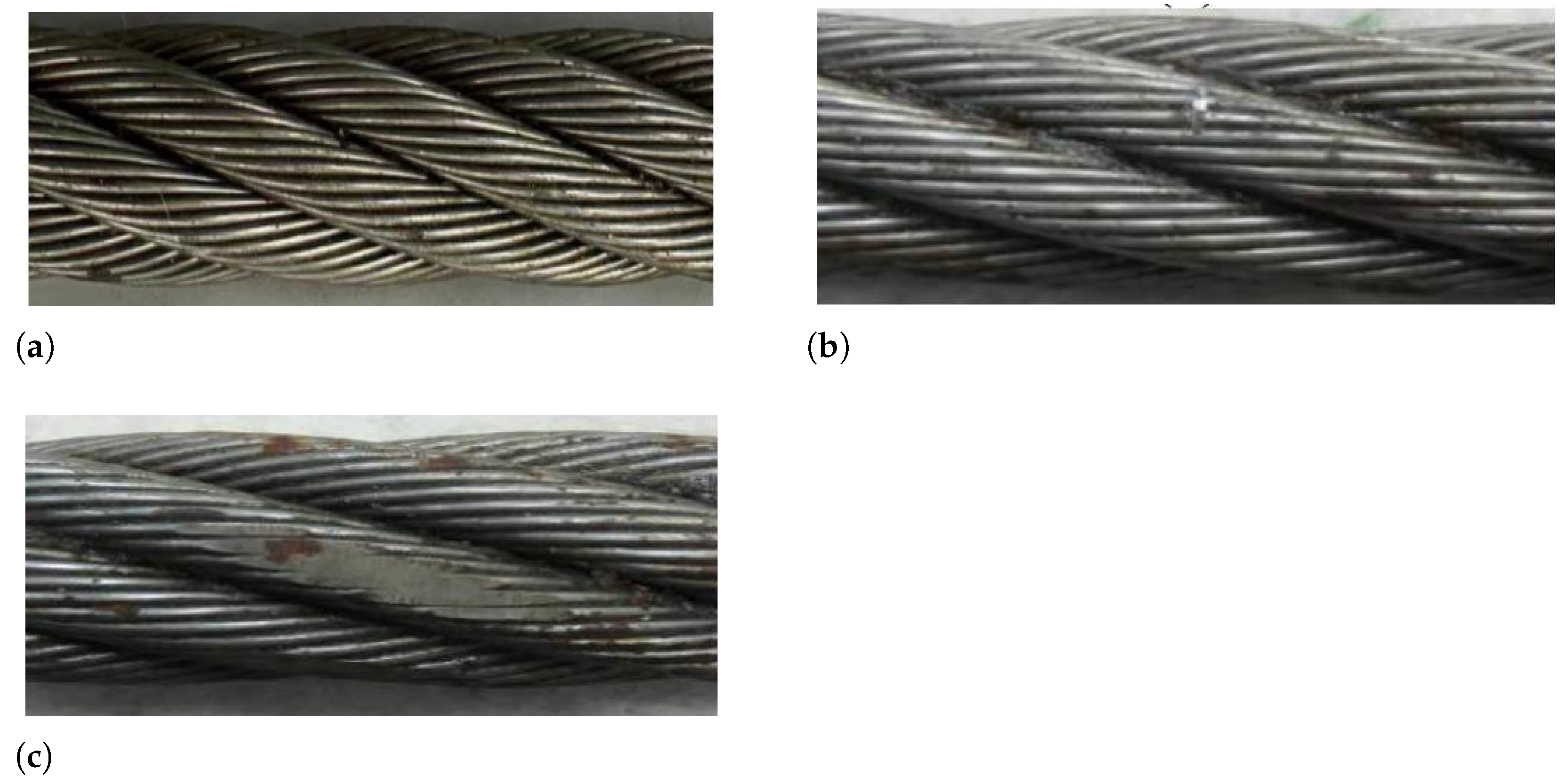
Throughout training, input images undergo augmentation and resizing before being fed into the CNNs. To reduce the influence of strand-related textures, spatial filtering based on strand inclination was applied to the raw MFL images, as shown in Figure 12c,d. The model was trained on these filtered images to preserve defect-related features while suppressing background textures. To enhance the robustness of the model, several data preprocessing and augmentation techniques were applied. First, additive Gaussian noise with zero mean and a standard deviation of $\sigma =0.01$ was added to the MFL signals during training to simulate real-world sensor noise. Second, to mimic partial occlusion or missing data in real scenarios, random rectangular masking was used to obscure 10–30% of the image area during augmentation. Third, beyond peak-to-peak normalization, each sensor channel was standardized using z-score normalization based on the channel’s mean and standard deviation across the dataset. This aimed to reduce hardware-specific signal variations.

Following this, predictions of bounding box information are generated based on anchor boxes. Subsequently, the loss function is employed to calculate the disparity between the predicted bounding boxes and the ground truth bounding boxes. During the testing phase, well-trained neural networks process input images with high efficiency, particularly benefiting from the one-to-one branch structure.

5.3. Evaluation Indicator

The commonly used evaluation metrics for object detection include precision (P), recall (R), and mean Average Precision ($mAP$). Precision denotes the probability that all positive samples detected by the model are actual positive samples, while recall represents the probability that the model detects positive samples within the actual positive samples. Following standard definitions in the literature [31], precision and recall are defined by Equations (6) and (7), respectively:

$$P={\displaystyle \frac{T_P}{T_P+F_P}}$$

(6)

$$R={\displaystyle \frac{T_P}{T_P+F_N}}$$

(7)

Here, $T_P$ is the number of correctly detected defective samples, $F_P$ is the number of non-defective samples falsely identified as defective, $F_N$ is the number of defective samples incorrectly recognized. Furthermore, $mAP$ is a comprehensive metric considering both precision (P) and recall (R). A higher $mAP$ value indicates a higher detection accuracy of the model. It is defined as:

$$mAP={\displaystyle \frac{{\sum }_{i=1}^n{\int }_0^1{P}_i\left(R_i\right)d{R}_i}{n}}$$

(8)

5.4. Results

As shown in

Table 3. The performance comparison of different methods. The best performance in each row is highlighted in bold.

Method	Precision (%)	Recall (%)	mAP@50 (%)
YOLOv5	75.5	72.8	71.9
YOLOv8	74.4	73.1	70.2
YOLOv10	68.9	70.6	67.3
YOLOv11	74.1	73.5	72.2
YOLOv9e	73.0	76.7	75.9

, we compare five YOLO-based detectors on our defect dataset. YOLOv9e achieves the highest recall (76.7%) and mAP@50 (75.9%), while YOLOv5 achieves the best precision (75.5%). This indicates that YOLOv9e provides more comprehensive detection coverage, whereas YOLOv5 is more conservative but confident in its predictions.

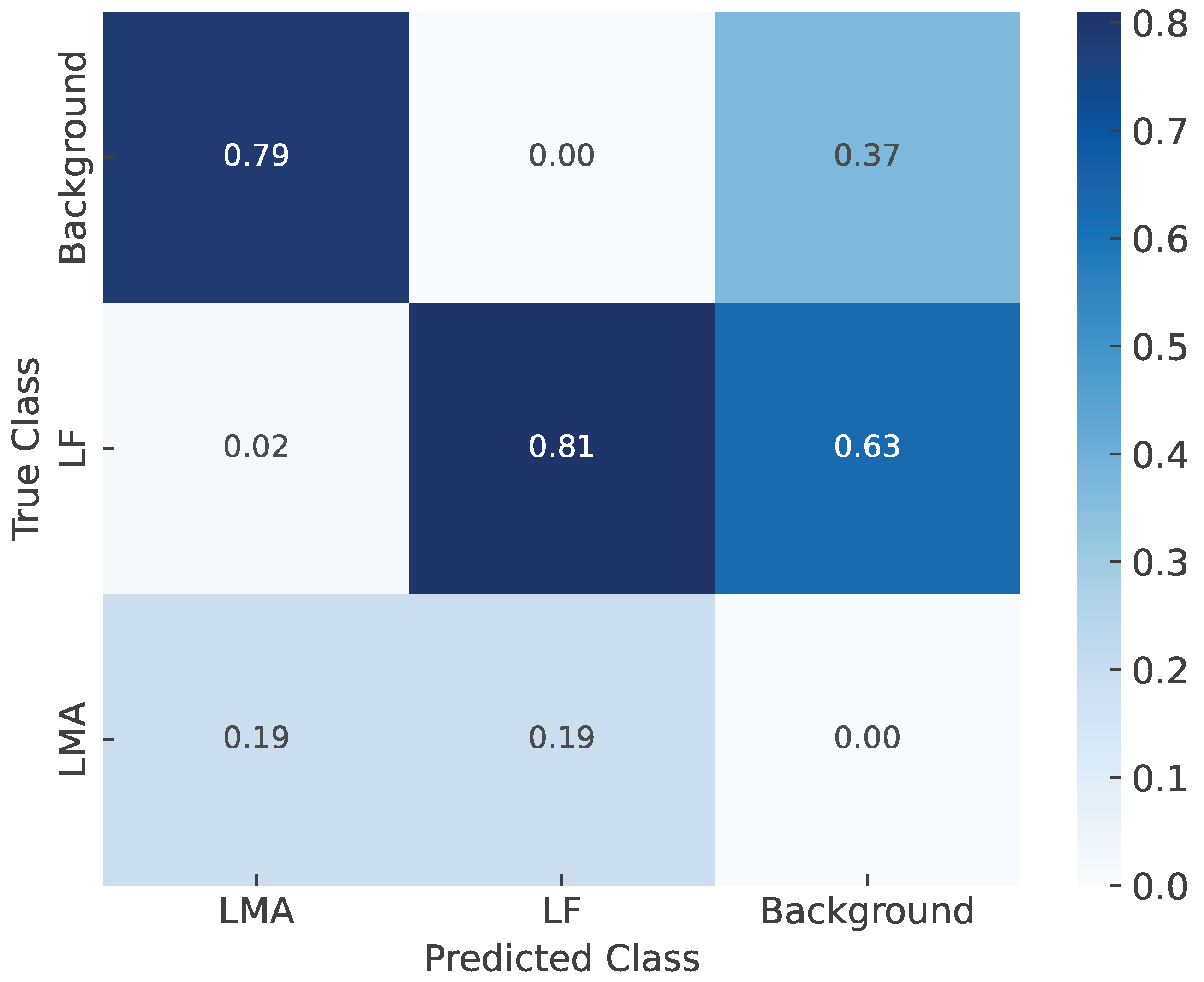
The performance gap can be attributed to the imbalance and complexity of the dataset, which contains 1678 LF and 981 LMA instances. LF defects are more frequent and typically localized, while LMA defects are more complex, spanning multiple strands with diffuse textures. YOLOv9e benefits from enhanced feature fusion and a deeper backbone, enabling better generalization across both defect types, particularly under class imbalance. In contrast, YOLOv10 underperforms across all metrics, likely due to insufficient feature resolution or limited adaptability to structural variation. YOLOv11 slightly outperforms YOLOv8 but does not surpass YOLOv9e, indicating that the ability to capture fine-scale textures and semantic cues remains critical for defect detection. These results highlight the importance of model architecture capacity and robustness to data distribution when deploying models for industrial inspection. Additionally, the confusion matrix illustrating classification outcomes for LMA, LF, and background classes is shown in Figure 14. The detection precision for LF defects is 81%, with 2% misclassified as LMA and 63% incorrectly identified as background, indicating substantial confusion with background regions. For LMA defects, the detection precision is 79%, with 37% misclassified as background. Interestingly, despite their larger spatial extent, LF defects show a higher false background rate, which may be attributed to their weaker texture contrast and smaller region size, making them more prone to being submerged in noisy background features. In contrast, LMA defects, although semantically more complex, may retain salient structures that the model can effectively learn. The background class itself suffers from severe misclassification, highlighting the challenge of effectively separating defect regions from complex backgrounds. To provide a more quantitative view of class-wise detection behavior,

Table 4. Class-wise performance metrics for defect detection. FPR values are estimated assuming the number of background instances is approximately equal to the total number of defect instances.

Class	TPR	FPR	FNR
LF	81%	32%	19%
LMA	37%	48%	63%

summarizes the True Positive Rate (TPR), False Positive Rate (FPR), and False Negative Rate (FNR) for the LF and LMA classes. TPR and FNR values are derived directly from the confusion matrix. Since the dataset lacks explicit annotations for background regions, FPR values are estimated under the assumption that the number of background instances is approximately equal to the total number of defect instances. This assumption enables approximate evaluation of how often background regions are incorrectly detected as defects. The estimated FPRs, 48% for LMA and 32% for LF, further support the observation that background confusion remains a critical challenge in defect localization.

To evaluate the generalization ability and robustness of our model under different data splits, we conducted a three-fold cross-validation. As shown in

Table 5. Performance of the YOLOv9e under 3-fold cross-validation. The best performance in each row is highlighted in bold.

Fold	Precision (%)	Recall (%)	mAP@50 (%)
1	76.9	75.8	73.8
2	74.2	76.3	74.5
3	73.7	75.7	72.2
Average	74.9	75.9	73.5

, the model consistently achieves high performance across all folds, with an average precision of 74.9%, recall of 75.9%, and mAP@50 of 73.5%. These results indicate that the model is not overfitting to a particular data split and maintains stable performance, thereby justifying the validity of the reported results.

5.5. Ablation Study

In this experiment, we investigate the impact of different learning rates on the performance of YOLOv9e for defect detection.

Table 6. Performance of YOLOv9e on defect detection dataset under different learning rates. The best results in each metric are highlighted in bold.

Learning Rate	Class	Precision (%)	Recall (%)	mAP@50 (%)	mAP@50:95 (%)
0.008	all	76.0	72.4	74.4	31.1
	LMA	79.3	75.2	81.1	41.5
	LF	72.7	69.5	67.8	20.6
0.006	all	74.7	77.6	73.9	30.9
	LMA	75.3	81.2	78.1	40.0
	LF	74.0	74.0	69.8	21.8
0.002	all	73.0	76.7	75.9	35.0
	LMA	77.5	78.2	80.5	46.2
	LF	68.6	75.1	71.3	23.7
0.001	all	75.5	74.5	74.7	30.4
	LMA	77.3	77.6	76.7	40.5
	LF	73.8	71.5	72.7	20.4
0.010	all	70.9	74.3	71.4	30.4
	LMA	71.3	79.2	75.7	40.7
	LF	70.5	69.5	67.2	20.1

presents results across various learning rates (0.008, 0.006, 0.002, 0.001, and 0.010), with the best values in each metric highlighted in bold. The results show that a learning rate of 0.002 yields the best overall performance in terms of mAP@50 (75.9%) and mAP@50:95 (35.0%), indicating that a lower learning rate facilitates better detection precision and generalization. In particular, for LMA defects, this setting achieves the highest mAP@50:95 (46.2%), likely due to the complex textures and varied scales of LMA defects, which require the model to capture subtle multi-scale features. A lower learning rate helps stabilize training, allowing the model to better handle these characteristics.

Conversely, higher learning rates (0.008 and 0.010) result in performance degradation across all metrics, especially mAP@50:95. This suggests that excessively high learning rates may cause instability during training, impairing the model’s ability to learn fine-grained defect patterns—especially critical for LMA detection. For LF defects, which are typically smaller and more localized, a learning rate of 0.006 achieves the highest mAP@50 (69.8%), suggesting that LF detection benefits from a moderate learning rate that balances convergence speed with accuracy. The dataset used in this study consists of 1678 LF and 981 LMA instances, collected from wire ropes in a controlled laboratory setting. Variations in defect size, texture, and boundary ambiguity influence the model’s sensitivity to the learning rate. Specifically, LF defects, being smaller and more localized, may require a slightly higher learning rate to avoid overfitting and encourage faster convergence. In contrast, LMA defects, with more complex patterns, benefit from the stability provided by a lower learning rate.

Overall, the study highlights that lower learning rates, such as 0.002, tend to yield better performance for complex defects like LMA, while higher learning rates may lead to convergence issues and performance degradation. These findings emphasize the importance of choosing an appropriate learning rate based on both the defect characteristics and dataset distribution to ensure model stability and optimal detection outcomes.

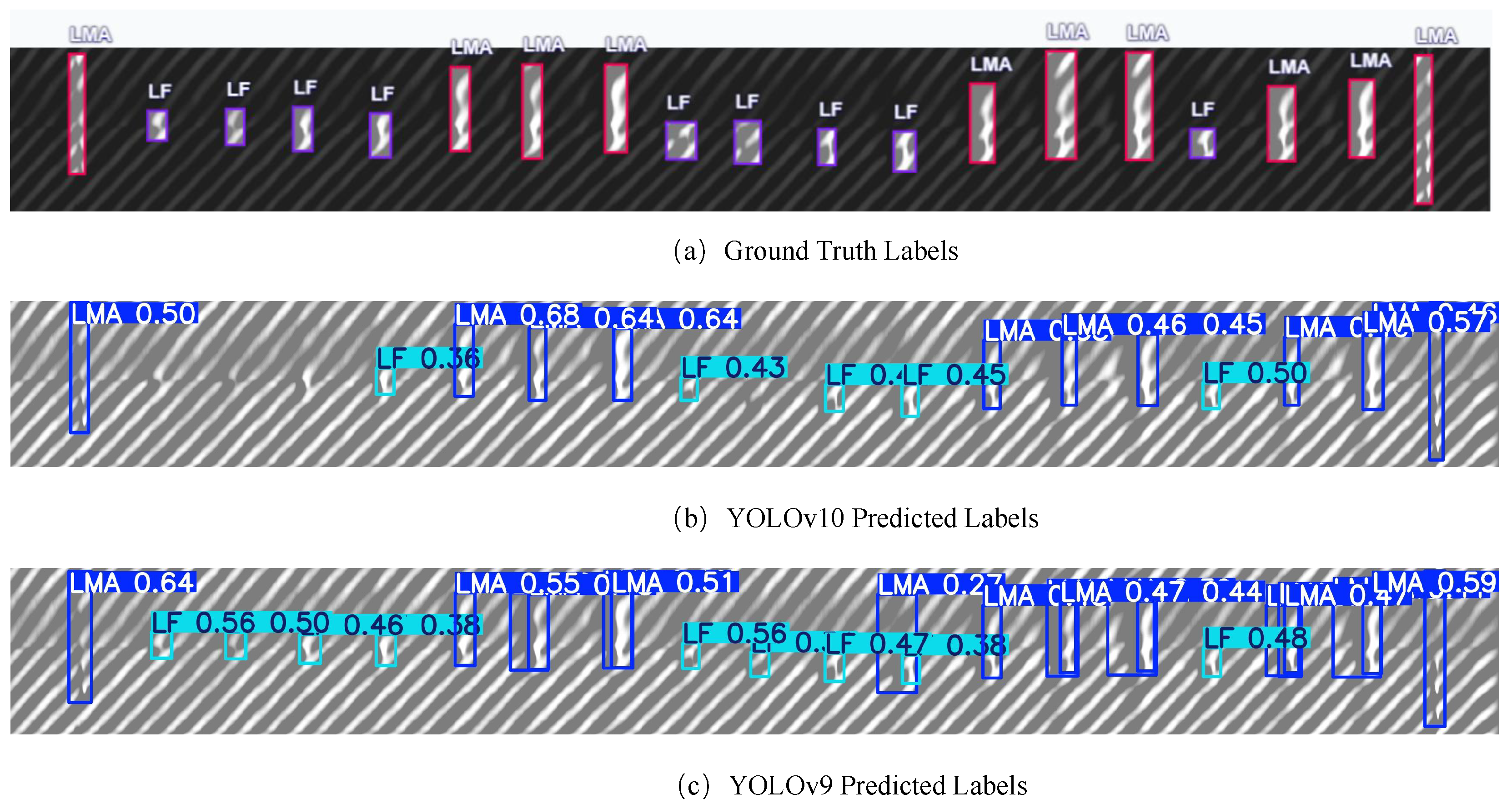
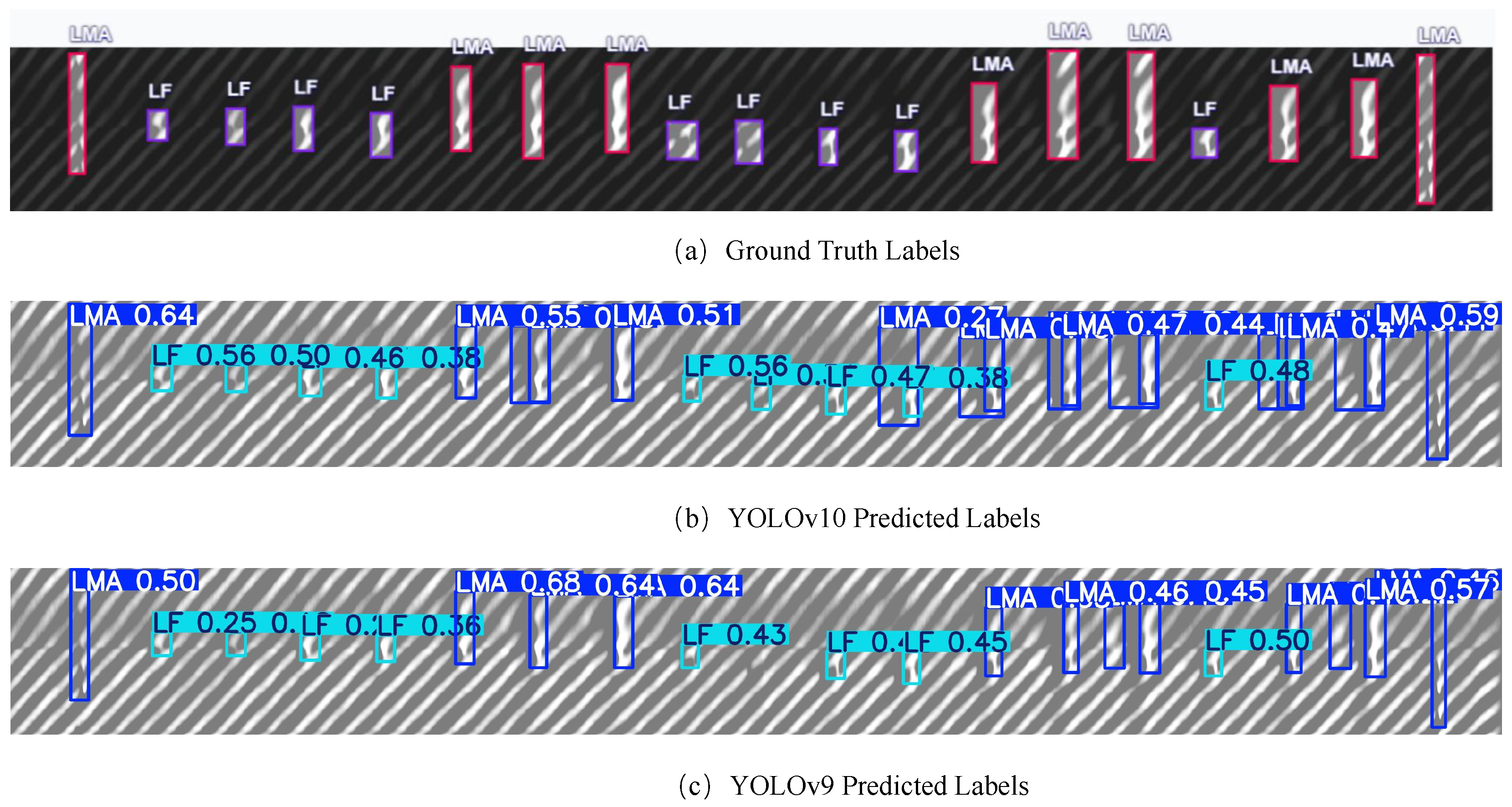
To further examine detection behavior under varying configurations, we compare YOLOv9e and YOLOv10 under different IoU and confidence thresholds, as illustrated in Figure 15 and Figure 16. Under default settings, YOLOv10 (Figure 15b) performs reliably in detecting large-scale LMA defects with high confidence and minimal redundancy. However, it fails to capture many small-scale LF instances, indicating limited sensitivity to fine-grained targets. In contrast, YOLOv9e (Figure 15c) detects most LF defects, benefiting from multi-scale feature extraction and enhanced spatial representation. Nonetheless, it suffers from redundant detections for LMA defects, especially when the defect spans a large area, resulting in overlapping bounding boxes. When the confidence threshold is reduced to 0.1 and the IoU threshold to 0.6 (Figure 16), YOLOv10 (Figure 16b) significantly improves its recall on LF instances, successfully capturing smaller defects. However, this improvement introduces redundant bounding boxes on LMA, mirroring the behavior of YOLOv9e under default settings. Under the same relaxed thresholds, YOLOv9e (Figure 16c) maintains high recall for both LMA and LF while effectively suppressing redundant detections on LMA, suggesting better spatial consistency and localization precision. These observations highlight the complementary characteristics of the two detectors and demonstrate that threshold tuning plays a critical role in balancing recall and redundancy. Moreover, they emphasize the need for adaptive post-processing strategies when applying object detectors to industrial defect datasets with mixed defect sizes and ambiguous boundaries.

To justify the necessity of deep neural networks for our defect detection task, we performed a cross-series ablation study on several YOLO architectures with varying depth and capacity: YOLOv5n (Nano), YOLOv9t (Shallow), YOLOv9s (Medium), and YOLOv9e (Deep). As shown in

Table 7. Cross-series depth ablation study on YOLO architectures. The best performance in each row is highlighted in bold.

Method	Depth Level	Precision (%)	Recall (%)	mAP@50 (%)
YOLOv5n	Nano	71.6	71.9	70.1
YOLOv9t	Shallow	71.7	72.7	70.0
YOLOv9s	Medium	73.0	77.5	72.1
YOLOv9e	Deep	73.0	76.7	75.9

, the detection performance improves consistently with the depth of the model. YOLOv9e achieves the highest mAP@50 (75.9%) and recall (76.7%), significantly outperforming shallower counterparts such as YOLOv5n (70.1%, 71.9%) and YOLOv9t (70.0%, 72.7%). These results demonstrate that deeper networks are more effective in capturing complex and subtle visual patterns present in pipeline defects, particularly under challenging conditions such as noisy backgrounds and low contrast features. This supports the adoption of deep architectures not only for improved robustness, but also for their superior feature extraction capacity, which is critical for detecting small LF defects.

Furthermore, we performed an ablation study to evaluate the impact of the Auxiliary Reversible Branch (ARB) in YOLOv9e. As shown in

Table 8. Ablation results of YOLOv9e with and without Auxiliary Reversible Branch. The best performance in each row is highlighted in bold.

Model	Precision (%)	Recall (%)	mAP@50 (%)
YOLOv9e (w/o ARB)	71.5	77.6	74.8
YOLOv9e (full)	73.0	76.7	75.9

, removing ARB leads to a drop in both precision and mAP@50, indicating that ARB enhances the model’s ability to localize and classify defects more accurately. Interestingly, the recall slightly increases without ARB, suggesting a more aggressive detection behavior, possibly at the cost of increased false positives.

5.6. Limitations and Future Work

While our current dataset supports reliable defect detection under controlled laboratory settings, it does not encompass certain real-world variations. Specifically, all MFL data were acquired under a fixed magnetization current and excitation configuration. Consequently, the model’s sensitivity to variations in magnetization strength could not be evaluated in this study. Similarly, the dataset was collected under stable indoor temperature conditions without explicit simulation or measurement of temperature-induced drift in Hall sensors, which may affect signal integrity in practical applications. Furthermore, our dataset focuses exclusively on clearly defined structural defects and does not include non-defect signal anomalies such as rust-induced distortions or material inconsistencies that may result in false positives. These aspects, including magnetization variability, thermal effects, and non-defect interference, are critical factors in real-world MFL inspection and will be addressed in future data collection and model evaluation.

6. Conclusions and Discussion

In summary, this study has demonstrated the effectiveness of preprocessing multi-channel one-dimensional magnetic flux leakage (MFL) signals and converting them into MFL images. This transformation facilitates two-dimensional defect localization and significantly improves the resolution and interpretability of defect analysis. By leveraging advanced deep learning algorithms, an effective real-time defect detection framework based on MFL technology was established, enhancing both the accuracy and efficiency of the detection process. The adoption of the enhanced YOLOv9e network enabled precise analysis of MFL images, delivering accurate localization and size estimation of detected defects. This approach markedly improves the performance of MFL-based inspection for steel wire ropes. Compared to traditional model-driven or handcrafted approaches, the proposed framework demonstrates clear advantages in terms of spatial resolution and background suppression, which make it well suited for deployment in complex industrial inspection environments.

References

1. Dwivedi, S.K.; Vishwakarma, M.; Soni, A. Advances and Researches on Non Destructive Testing: A Review. Mater. Today Proc. 2018, 5, 3690–3698. [Google Scholar] [CrossRef]
2. Mazurek, P. A comprehensive review of steel wire rope degradation mechanisms and recent damage detection methods. Sustainability 2023, 15, 5441. [Google Scholar] [CrossRef]
3. Rostami, J.; Tse, P.W.; Yuan, M. Detection of broken wires in elevator wire ropes with ultrasonic guided waves and tone-burst wavelet. Struct. Health Monit. 2020, 19, 481–494. [Google Scholar] [CrossRef]
4. Chakhlov, S.; Anpilogov, P.; Batranin, A.; Osipov, S.; Zhumabekova, S.; Yadrenkin, I. Generation and analysis of wire rope digital radiographic images. Iop Conf. Ser. Mater. Sci. Eng. 2016, 132, 012008. [Google Scholar] [CrossRef]
5. Feng, B.; Deng, K.; Wang, S.; Chen, S.; Kang, Y. Theoretical Analysis on the Distribution of Eddy Current in Motion-Induced Eddy Current Testing and High-Speed MFL Testing. J. Nondestruct. Eval. 2022, 41, 59. [Google Scholar] [CrossRef]
6. Xia, H.; Yan, R.; Wu, J.; He, S.; Zhang, M.; Qiu, Q.; Zhu, J.; Wang, J. Visualization and quantification of broken wires in steel wire ropes based on induction thermography. IEEE Sens. J. 2021, 21, 18497–18503. [Google Scholar] [CrossRef]
7. Xu, L.; Hu, J. A method of defect depth recognition in active infrared thermography based on GRU networks. Appl. Sci. 2021, 11, 6387. [Google Scholar] [CrossRef]
8. Xin, H.; Cheng, L.; Diender, R.; Veljkovic, M. Fracture acoustic emission signals identification of stay cables in bridge engineering application using deep transfer learning and wavelet analysis. Adv. Bridge Eng. 2020, 1, 6. [Google Scholar] [CrossRef]
9. Juraszek, J. Residual magnetic field for identification of damage in steel wire rope. Arch. Min. Sci. 2019, 64, 79–92. [Google Scholar] [CrossRef]
10. Liu, S.; Sun, Y.; Jiang, X.; Kang, Y. A new MFL imaging and quantitative nondestructive evaluation method in wire rope defect detection. Mech. Syst. Signal Process. 2022, 163, 108156. [Google Scholar] [CrossRef]
11. Peng, X.; Anyaoha, U.; Liu, Z.; Tsukada, K. Analysis of magnetic-flux leakage (MFL) data for pipeline corrosion assessment. IEEE Trans. Magn. 2020, 56, 6200315. [Google Scholar] [CrossRef]
12. Li, F.; Feng, J.; Zhang, H.; Liu, J.; Lu, S.; Ma, D. Quick reconstruction of arbitrary pipeline defect profiles from MFL measurements employing modified harmony search algorithm. IEEE Trans. Instrum. Meas. 2018, 67, 2200–2213. [Google Scholar] [CrossRef]
13. Peng, L.; Huang, S.; Wang, S.; Zhao, W. An element-combination method for arbitrary defect reconstruction from MFL signals. In Proceedings of the 2020 IEEE International Instrumentation and Measurement Technology Conference (I2MTC), Dubrovnik, Croatia, 25–28 May 2020; pp. 1–6. [Google Scholar]
14. Long, Y.; Huang, S.; Peng, L.; Wang, S.; Zhao, W. A characteristic approximation approach to defect opening profile recognition in magnetic flux leakage detection. IEEE Trans. Instrum. Meas. 2021, 70, 6003912. [Google Scholar] [CrossRef]
15. Tan, X.; Zhang, J. Evaluation of Composite Wire Ropes Using Unsaturated Magnetic Excitation and Reconstruction Image with Super-Resolution. Appl. Sci. 2018, 8, 767. [Google Scholar] [CrossRef]
16. Pan, J.; Gao, L. A novel method for defects marking and classifying in MFL inspection of pipeline. Int. J. Press. Vessel. Pip. 2023, 202, 104892. [Google Scholar] [CrossRef]
17. Liu, R.; Shao, Z.; Sun, Q.; Yu, Z. Defect detection and 3d reconstruction of complex urban underground pipeline scenes for sewer robots. Sensors 2024, 24, 7557. [Google Scholar] [CrossRef]
18. Wu, Z.; Deng, Y.; Liu, J.; Wang, L. A reinforcement learning-based reconstruction method for complex defect profiles in MFL inspection. IEEE Trans. Instrum. Meas. 2021, 70, 2506010. [Google Scholar] [CrossRef]
19. Tu, F.; Wei, M.; Liu, J. A coupling model of multi-feature fusion and multi-machine learning model integration for defect recognition. J. Magn. Magn. Mater. 2023, 568, 170395. [Google Scholar] [CrossRef]
20. Chen, P.; Li, R.; Fu, K.; Zhong, Z.; Xie, J.; Wang, J.; Zhu, J. A cascaded deep learning approach for detecting pipeline defects via pretrained YOLOv5 and ViT models based on MFL data. Mech. Syst. Signal Process. 2024, 206, 110919. [Google Scholar] [CrossRef]
21. Wang, G.; Su, Y.; Lu, M.; Chen, R.; Sun, X. Multi-modality hierarchical attention networks for defect identification in pipeline MFL detection. Meas. Sci. Technol. 2024, 35, 116107. [Google Scholar] [CrossRef]
22. Dutta, S.M.; Ghorbel, F.H.; Stanley, R.K. Dipole modeling of magnetic flux leakage. IEEE Trans. Magn. 2009, 45, 1959–1965. [Google Scholar] [CrossRef]
23. Ren, S.; He, K.; Girshick, R.; Sun, J. Faster r-cnn: Towards real-time object detection with region proposal networks. Adv. Neural Inf. Process. Syst. 2015, 28. Available online: https://proceedings.neurips.cc/paper_files/paper/2015/file/14bfa6bb14875e45bba028a21ed38046-Paper.pdf (accessed on 20 July 2025). [CrossRef]
24. He, K.; Gkioxari, G.; Dollár, P.; Girshick, R. Mask r-cnn. In Proceedings of the IEEE International Conference on Computer Vision, Venice, Italy, 22–29 October 2017; pp. 2961–2969. [Google Scholar]
25. Chai, B.; Nie, X.; Zhou, Q.; Zhou, X. Enhanced cascade R-CNN for multiscale object detection in dense scenes from SAR images. IEEE Sens. J. 2024, 24, 20143–20153. [Google Scholar] [CrossRef]
26. Redmon, J.; Divvala, S.; Girshick, R.; Farhadi, A. You only look once: Unified, real-time object detection. In Proceedings of the IEEE Conference on Computer Vision and Pattern Recognition, Las Vegas, NV, USA, 26 June–1 July 2016; pp. 779–788. [Google Scholar]
27. Wang, H.; Qian, H.; Feng, S.; Wang, W. L-SSD: Lightweight SSD target detection based on depth-separable convolution. J. Real-Time Image Process. 2024, 21, 33. [Google Scholar] [CrossRef]
28. Wu, B.; Iandola, F.; Jin, P.H.; Keutzer, K. Squeezedet: Unified, small, low power fully convolutional neural networks for real-time object detection for autonomous driving. In Proceedings of the IEEE Conference on Computer Vision and Pattern Recognition Workshops, Honolulu, HI, USA, 21–26 July 2017; pp. 129–137. [Google Scholar]
29. Tian, Z.; Shen, C.; Chen, H.; He, T. Fcos: Fully convolutional one-stage object detection. In Proceedings of the IEEE/CVF International Conference on Computer Vision, Seoul, Republic of Korea, 27 October–2 November 2019; pp. 9627–9636. [Google Scholar]
30. Tan, M.; Pang, R.; Le, Q.V. Efficientdet: Scalable and efficient object detection. In Proceedings of the IEEE/CVF Conference on Computer Vision and Pattern Recognition, Seattle, WA, USA, 14–19 June 2020; pp. 10781–10790. [Google Scholar]
31. Wang, G.; Chen, Y.; An, P.; Hong, H.; Hu, J.; Huang, T. UAV-YOLOv8: A small-object-detection model based on improved YOLOv8 for UAV aerial photography scenarios. Sensors 2023, 23, 7190. [Google Scholar] [CrossRef] [PubMed]
Figure 1. Schematic of excitation structure and detect sensor.
Jsan 14 00080 g001
Figure 2. Schematic of the dipole model on a wire rope.
Jsan 14 00080 g002
Figure 3. Cylindrical defect magnet dipole model (a) 3D view, (b) top view.
Jsan 14 00080 g003
Figure 4. Normalized radial component H R of leakage magnetic field spatial distribution (a) 3D view, (b) top view.
Jsan 14 00080 g004
Figure 5. Architecture of YOLOv9.
Jsan 14 00080 g005
Figure 6. Schematic view of system structure.
Jsan 14 00080 g006
Figure 7. Photographic view of system structure.
Jsan 14 00080 g007
Figure 8. Experimental diagram (a) Photographic view of Hall sensor array, (b) diagram of experimental assembly.
Jsan 14 00080 g008
Figure 9. Flaw diagram of leakage magnetic field acquisition system.
Jsan 14 00080 g009
Figure 10. Experimental diagram (a) Photographic view of the steel wire rope, (b) typical LF defect diagram, (c) typical LMA defect diagram.
Jsan 14 00080 g010
Figure 11. Typical 3D MFL images (a) Schematic diagram of MFL image, (b) raw MFL image, (c) processed MFL image.
Jsan 14 00080 g011
Figure 12. Typical 2D MFL images (a) MFL image without defect, (b) MFL image with defects, (c) texture-removed MFL image without defect, (d) texture-removed MFL image with defects.
Jsan 14 00080 g012
Figure 13. Boxplot of defect area distributions for LMA and LF classes, showing clear intra-class and inter-class variability.
Jsan 14 00080 g013
Figure 14. Confusion matrix of all the prediction results.
Jsan 14 00080 g014
Figure 15. Results of YOLO with default IoU and confidence thresholds.
Jsan 14 00080 g015
Figure 16. YOLO results with confidence threshold = 0.1 and IoU threshold = 0.6.
Jsan 14 00080 g016