
Compressive Sensing in Power Engineering: A Comprehensive Survey of Theory and Applications, and a Case Study

 , ,
, ,  ,
,
Abstract
1. Introduction
- High-Volume Data Transmission: Traditional data acquisition and transmission techniques require full Nyquist-rate sampling, leading to excessive bandwidth usage, high storage requirements, and communication congestion in smart grids.
- Bandwidth and Latency Constraints: Many power system applications, such as fault detection, real-time state estimation, and condition monitoring, require low-latency and high-fidelity data transmission. However, conventional compression methods introduce computational delays, making them unsuitable for real-time processing.
- Energy-Efficient Data Processing: In large-scale sensor networks, such as PMUs and IoT-based smart grid sensors, the energy cost of continuous data transmission is high. Efficient data acquisition strategies are needed to reduce transmission overhead while ensuring robust monitoring capabilities.
- Scalability and Resource Constraints: As smart grids expand, the increasing number of sensors and IoT devices exacerbates the problem of real-time data management, requiring lightweight, scalable solutions for sensor data acquisition.
- Lossy Compression: Techniques like Singular Value Decomposition (SVD), Principal Component Analysis (PCA), and Symbolic Aggregate Approximation (SAX) reduce data size by discarding less significant information. These are suitable for applications where a trade-off between size and quality is acceptable, such as image or video compression.
- Lossless Compression: Methods like Huffman coding and LZ algorithms preserve all original data, ensuring perfect reconstruction but often requiring extensive computational resources.
- Sparsity: Signals with many near-zero coefficients in a transform domain (e.g., wavelet or Fourier domain).
- Random Projections: Encoding sparse signals through measurement matrices that satisfy the Restricted Isometry Property (RIP).
- Efficient Recovery Algorithms: Reconstruction of the original signal using techniques like ℓ1-minimization.
2. Motivation and Contributions
- (a)
- A Comprehensive Theoretical Overview: We present a robust foundation of CS principles, covering key aspects like sensing matrices, measurement bases, and recovery algorithms. This theoretical grounding aids in understanding how CS can be strategically applied to real-world grid applications.
- (b)
- Applications in Power Engineering: We examine major applications of CS across power engineering scenarios, including Advanced Metering Infrastructure, state estimation, fault detection, fault localization, outage identification, harmonic sources identification, power quality detection, condition monitoring, and IoT-based smart grid monitoring. By detailing these use cases, we highlight how CS addresses specific challenges such as data sparsity, transmission efficiency, and communication constraints, ultimately offering new pathways for efficient grid operation.
- (c)
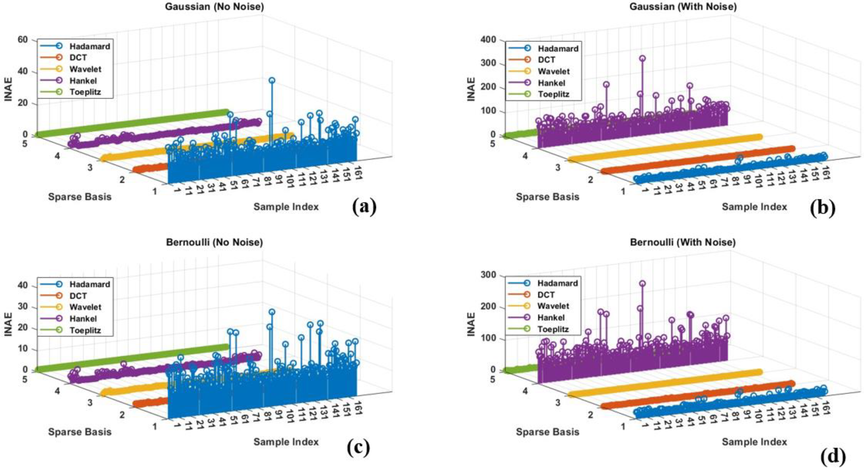
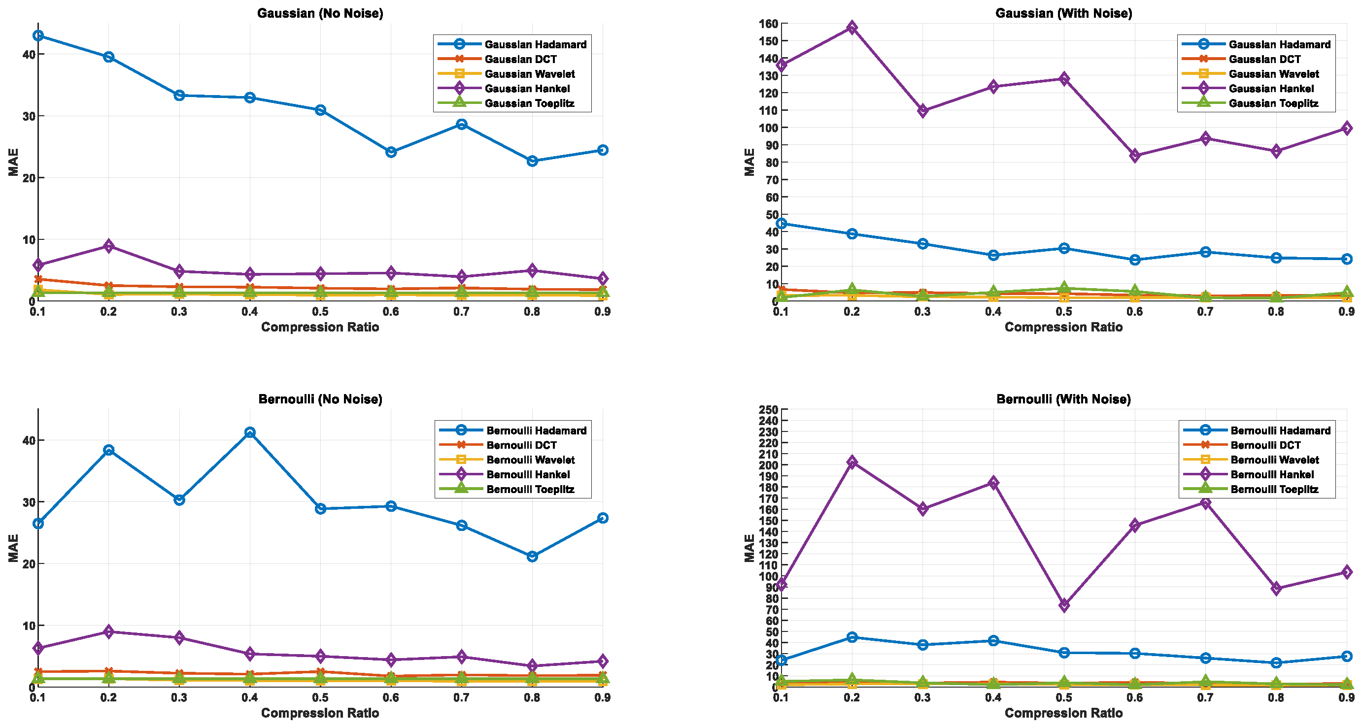
- A Case Study: We evaluate the effectiveness of various sparse bases and measurement matrices for smart meter data recovery under different compression ratios and noise conditions. This study systematically examines the impact of compression ratios on reconstruction accuracy in both noise-free and noisy environments, providing practical insights into designing robust CS-based compression techniques for power grid data. The findings contribute to optimizing data acquisition and transmission strategies, enhancing efficiency in power system monitoring and operation.
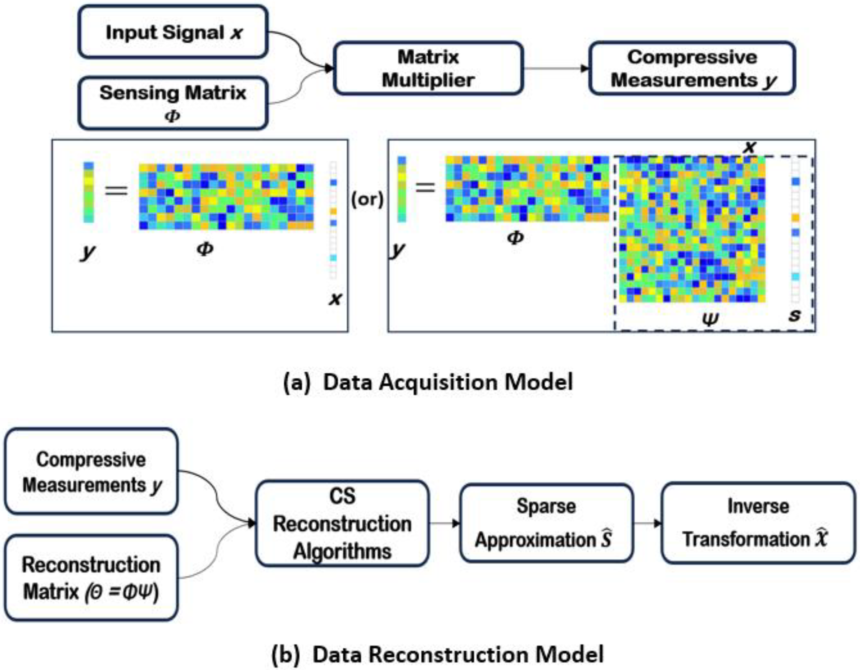
3. Compressive Sensing Paradigm
- Measurement Matrix/Sensing Matrix (Φ):
- Sparse Basis/Dictionary Matrix (Ψ):
- Reconstruction Matrix (Θ = ΦΨ):
- (i)
- l0 Norm Minimization:
- (ii)
- l1 Norm Minimization:
- (iii)
- l2 Norm Minimization:
- (i)
- Sparsity: For CS techniques to be effective, signals need to be sparse or nearly sparse. Sparsity refers to having few non-zero coefficients, while near sparsity means that the coefficients are close to zero. A signal x is said to be k-sparse in the Ψ domain if it can be represented with only k non-zero coefficients when transformed by Ψ.
- (ii)
- Incoherence: This broadens the time–frequency relationship, suggesting that objects with a sparse representation in one domain, symbolized by Ψ, are distributed over the domain of acquisition, just as a singular pulse or spike in the time domain disperses across the frequency domain [4]. Incoherence is a measure of the dissimilarity between the measurement basis ϕ and the sparsity basis ψ. For precise reconstruction in CS, these bases must be incoherent with each other. The mutual coherence μ is a statistic that quantifies the maximum correlation between the elements of these two matrices and is given by Equation (13) [20]:
- (i)
- Restricted Isometry Property (RIP): The reconstruction matrix Θ must satisfy the RIP condition to ensure the preservation of the geometric properties of a sparse signal during transformation and measurement. RIP maintains the distances (Euclidian or l2 norm) between sparse signals, preventing them from being too closely mapped, which facilitates accurate reconstruction. Formally, a matrix obeys the RIP of order ‘k’ if the restricted isometry constant δk satisfies Equation (15) [22],for all k-sparse vectors ‘x’. The RIP ensures that all subsets of ‘k’ columns taken from the matrix are nearly orthogonal. RIP enables compressive sensing algorithms to embed sufficient information within a reduced number of samples, allowing for accurate reconstruction and robustness against noise. It provides a deterministic guarantee for the accurate reconstruction of sparse signals, even in the presence of noise interference.
4. Measurement Matrix and Sparse Basis Matrix
4.1. Measurement Matrices
4.1.1. Random Matrices
4.1.2. Deterministic and Structured Matrices
4.1.3. Chaotic Matrix
4.2. Sparse Basis Matrices
4.2.1. Fixed Sparse Basis Matrices
4.2.2. Over-Complete Dictionaries
4.2.3. Data-Driven Dictionaries
5. Signal Reconstruction Algorithms
- i.
- ii.
- iii.
- Iterative/Thresholding Algorithms: These methods iteratively refine the solution through thresholding to promote sparsity and are computationally efficient and suitable for large-scale problems, but their performance depends on parameter selection and preconditioning [37,61,62,63] (e.g., ISTA, FISTA).
- iv.
- v.
- vi.
- vii.
6. Performance Metrics for Evaluation
- (a)
- Sparsity: For a signal x with N samples, if it is k-sparse in a sparse basis, then k represents the count of non-zero coefficients, which is significantly less than N. This means N−k coefficients can be discarded with minimal impact on the signal’s critical information. The percentage sparsity (fraction of non-zero coefficients) is given as in Equation (16):
- (b)
- Compression Ratio (CR)
- (c)
- Error Metrics: RE, MSE, RMSE, NMSE, MAE, INAE
- Reconstruction error (RE), also known as recovery error, is the ratio of the norm of the difference between the original signal and the reconstructed signal divided by the norm of the original signal. RE is given in Equation (18):
- Mean square error (MSE) measures the average magnitude of the squared difference between the original signal and the recovered signal. MSE given as in Equation (19) is a widely used metric to assess the quality of reconstruction:
- Root Mean Square (RMSE) measures the square root of the MSE and is given as in Equation (20):
- Normalized Mean Squared Error (NMSE) is given as in Equation (21):
- Mean Absolute Error (MAE) measures the average absolute difference between the original signal and the reconstructed signal and is given as in Equation (22):
- Integrated Normalized Absolute Error (INAE) evaluates the normalized cumulative reconstruction error over all elements of the signal and is given as in Equation (23):
- (d)
- Signal-to-Noise Ratio (SNR)
- (e)
- Computation Time (CT)
- (f)
- Recovery Time (RT)
- (g)
- Reconstruction/Recovery Success Rate (RSR) and Failure Rate
- (h)
- Complexity
- (i)
- Correlation
7. Compressive Sensing in Power Engineering
7.1. Advanced Metering Infrastructure (AMI)
- Step 1: The initial vector required for generating the measurement matrix is securely transmitted via a physical layer security scheme based on channel reciprocity in a time–division duplex (TDD) mode.
- Step 2: Upon receiving the compressed signal, the DCU reconstructs it using CS and evaluates the residual error.
- Step 3: The residual error is used as a test statistic in hypothesis testing to distinguish legitimate signals from intrusion attempts.
7.2. Wide-Area Measurement Systems (WAMSs)

| Wide-Area Measurement Systems (WAMS) | ||||
| Ref. | Sensing /Measurement Matrix | Recovery Algorithm | Sparse Basis | Inferences/Comments |
| [92] | Random | Modified Subspace Pursuit | Partial Fourier/DCT | CS-based PMU data recosntruction. |
| [93] | Random | Subspace Pursuit | Fourier Transform | CS-based PMU data recosntruction. |
| [96] | Random | - | Wavelet Transform | Adaptive compression combining clustering analysis with multiscale Principal Component Analysis (MSPCA). Leverages both spatial and temporal sparsity. |
7.3. State Estimation (SE) and Topology Identification (TI)
- Complexity of Distribution Networks: SE in distribution networks is less studied compared to transmission systems, primarily due to its radial structure with multiple feeders and branches, unbalanced loads, and limited measurements.
- Nonlinear Relationships: Power flow relationships between voltage states and other grid variables are highly nonlinear, complicating traditional SE approaches.
- Impact of Renewable Integration: The variability introduced by distributed generation (DG) creates correlated data patterns, necessitating adaptive estimation techniques.
- High Computational Costs: Traditional model-based methods rely on physical parameters, such as Distribution Factors (DFs) and Injection Shift Factors (ISFs), but face high computational costs and uncertainties in real-time applications [16]. Methods for calculating DFs include model-based, data-driven non-sparse, and data-driven sparse estimation. Model-based methods face uncertainties and high computational costs, while data-driven models adapt better to changing conditions [97]. However, non-sparse methods can contribute to the curse of dimensionality.
7.4. Fault Detection (FD), Fault Localization (FL) and Outage Identification (OI)
- Dynamic Range and Clustered Sparsity: Variations in fault signal magnitudes and clustered outage patterns complicate recovery, requiring advanced algorithms to handle these structured sparsity challenges [110].
7.5. Harmonic Source Identification (HSI) and Power Quality Detection (PQD)
- Continuous Sampling and Compression: Signals are compressed using sparse random matrices to reduce data volume.
- Dynamic Signal Recovery: Homotopy Optimization with Fundamental Filter (HO-FF) iteratively updates sparse solutions without re-solving the entire problem, enhancing computational efficiency.
- Harmonic Spectrum Correction: Single-peak spectral interpolation mitigates spectral leakage and phase errors, ensuring accurate recovery.
- Feedback Mechanism: Dynamically adjusts the compressed sampling ratio to adapt to fluctuating harmonic conditions.
7.6. Condition Monitoring (CM) of Machines
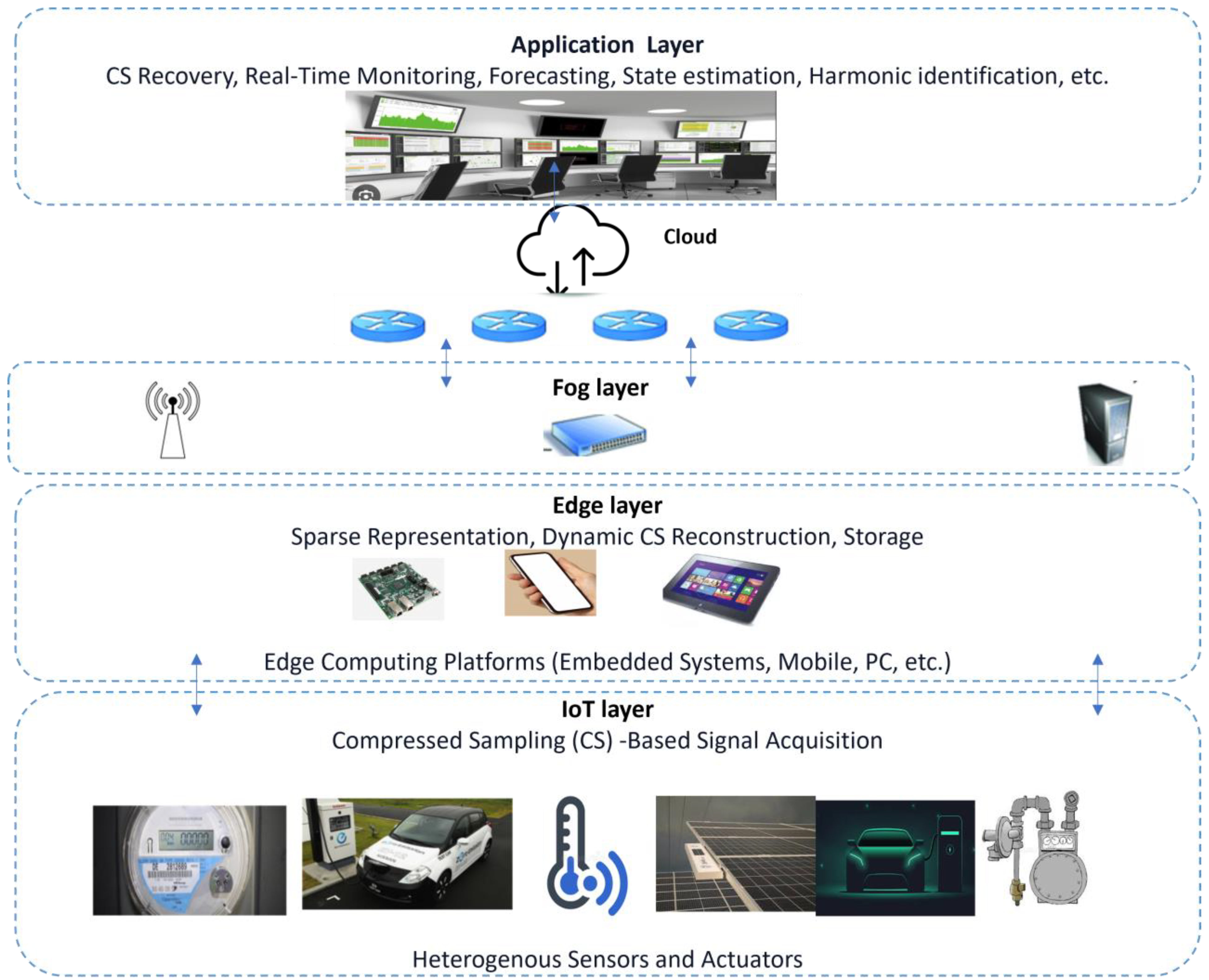
7.7. Compressive Sensing for IoT-Based Smartgrid Monitoring
8. Case Study: Performance Analysis of Compressive Sensing in Data Recovery
8.1. Effect of Compression Ratio (CR)
8.2. Sparse Basis Performance
8.3. Choice of Measurement Matrices
9. Conclusion and Emerging Research Opportunities in Compressive Sensing
- i.
- Measurement Matrix Design and Optimization: Adaptive and weighted measurement strategies can achieve this by focusing on the most informative aspects of the signal. Utilizing machine learning techniques, such as genetic algorithms, to design measurement matrices offers adaptive solutions tailored to dynamic signal behaviors [147,148].
- ii.
- Adaptive and Optimal Basis Selection: Developing algorithms that dynamically select the optimal sparsity basis is crucial for adapting to fluctuating system conditions. Data-driven and tensor-based methods can tailor the sparsity basis by analyzing inherent system characteristics, ensuring efficient signal representation and reconstruction. Incorporating advanced preprocessing techniques, such as noise filtering and decorrelation, into CS workflows can significantly enhance signal quality without compromising essential features required for accurate analysis and reconstruction [15,149]. The combination of CS with techniques like the Discrete Cosine Transform (DCT) and Amended Intrinsic Chirp Separation (AIChirS) to precisely reconstruct overlapping non-stationary signals can be explored [150].
- iii.
- Recovery algorithms: Research efforts should continue to refine recovery algorithms, striving for excellence in terms of speed, efficiency, robustness, handling structured and non-sparse signals.
- iv.
- Scalability and Energy Efficiency studies in Large-Scale Systems: As the number of connected devices increases, scalability becomes paramount [145,148]. CS can enhance data storage efficiency in large-scale frameworks like China’s UPIoT and the emerging energy internet [150]. By effectively compressing data, CS reduces storage requirements and facilitates seamless data management. Shifting computational demands from resource-constrained IoT devices to robust gateways can lead to significant energy savings. In smart grids, joint sparse recovery techniques mitigate communication network burdens by simultaneously recovering multiple sparse vectors, thereby optimizing energy consumption [151,152]. Designing lightweight CS solutions optimized for resource-constrained devices, such as IoT nodes and smart sensors, is essential [153,154,155]. Employing fixed-point arithmetic on FPGAs and optimizing GPU kernels can achieve a balance between performance and power consumption, ensuring efficient CS operations on edge devices [156]. In asset monitoring and vegetation management, employing CS-based image processing with fewer UAV sensors minimizes energy usage and extends the operational lifespan of deployed devices, contributing to sustainable and cost-effective monitoring solutions [157]. Block Compressed Sensing (BCS), which segments large datasets into smaller blocks, enhances processing speed and system efficiency, making it feasible for large-scale power systems.
- v.
- Spatio-Temporal Models: Developing hierarchical CS frameworks by integrating Distributed Compressive Sensing (DCS) and Dynamic Distributed Compressive Sensing (DDCS) can improve data handling from complex sources such as multi-bus grids, UAV networks, and smart cities [149,158]. These models enhance data reconstruction accuracy and efficiency in large-scale power systems. Investigating spatio-temporal CS techniques can enhance large-scale monitoring systems by exploiting spatial correlations to reduce data redundancy while maintaining high reconstruction accuracy in geographically distributed networks [149].
- vi.
- CS integration with Cloud and Edge Computing: Integrating compressive data gathering with link scheduling can further reduce energy consumption and network traffic in applications like Advanced Metering Infrastructure (AMI) and Smart Grids by focusing on data reduction and security. Hybrid Cloud-Edge Architectures enhances the scalability and responsiveness of CS applications in power engineering, balancing computational loads between local devices and centralized cloud resources.
- vii.
- CS fusion with Deep Neural Networks: Combining CS with deep learning can create adaptive and intelligent systems capable of simultaneous classification, forecasting, and reconstruction [87,88]. Such systems hold significant promise for applications like fault detection (FD) and Power Quality Detection (PQD), leveraging the strengths of both CS and deep learning for more robust and accurate monitoring solutions.
- viii.
- Security and Privacy Enhancements: Advancing CS-based encryption methods, where sensing matrices also serve as encryption keys, can enhance data security in critical applications such as AMI and sensitive fields like medical data systems [159,160]. This dual purpose use of sensing matrices offers a novel approach to securing transmitted data without additional encryption overhead. Expanding federated CS frameworks to process sensitive data locally while incorporating robust security protocols, such as Quantum Key Distribution (QKD), can safeguard distributed systems against sophisticated cyber threats [161].
- ix.
- Quantum Computing Integration: Employing quantum algorithms, such as the Quantum Fourier Transform (QFT) and Harrow–Hassidim–Lloyd (HHL) algorithm, can significantly accelerate sparse recovery and matrix operations [162]. This is particularly promising for real-time grid monitoring and renewable energy forecasting in resource-intensive applications. Exploring parallel computing, distributed algorithms, and hardware acceleration can address the computational demands of CS-based state estimations in expansive grids.
Author Contributions
Funding
Data Availability
Conflicts of Interest
References
- Wen, L.; Zhou, K.; Yang, S.; Li, L. Compression of Smart Meter Big Data: A Survey. Renew. Sustain. Energy Rev. 2018, 91, 59–69. [Google Scholar] [CrossRef]
- Li, H.; Mao, R.; Lai, L.; Qiu, R.C. Compressed Meter Reading for Delay-Sensitive and Secure Load Report in Smart Grid. In Proceedings of the First IEEE International Conference on Smart Grid Communications, Gaithersburg, MD, USA, 4–6 October 2010; pp. 114–119. [Google Scholar] [CrossRef]
- Louie, R.H.Y.; Hardjawana, W.; Li, Y.; Vucetic, B. Distributed Multiple-Access for Smart Grid Home Area Networks: Compressed Sensing with Multiple Antennas. IEEE Trans. Smart Grid 2014, 5, 2938–2946. [Google Scholar] [CrossRef]
- Candès, E.J.; Wakin, M.B. An Introduction to Compressive Sampling. IEEE Signal Process. Mag. 2008, 25, 21–30. [Google Scholar] [CrossRef]
- Donoho, D.L. Compressed Sensing. IEEE Trans. Inf. Theory 2006, 52, 1289–1306. [Google Scholar] [CrossRef]
- Candès, E.J. The Restricted Isometry Property and Its Implications for Compressed Sensing. Compt. Rendus Math. 2008, 346, 589–592. [Google Scholar] [CrossRef]
- Arie, R.; Brand, A.; Engelberg, S. Compressive Sensing and Sub-Nyquist Sampling. IEEE Instrum. Meas. Mag. 2020, 23, 94–101. [Google Scholar] [CrossRef]
- Machidon, A.L.; Pejović, V. Deep Learning for Compressive Sensing: A Ubiquitous Systems Perspective. Artif. Intell. Rev. 2023, 56, 3619–3658. [Google Scholar] [CrossRef]
- Chen, X.; Zhang, J.; Wang, X.; Han, G.; Xie, J. A Sub-Nyquist Rate Compressive Sensing Data Acquisition Front-End. IEEE J. Emerg. Sel. Top. Circuits Syst. 2012, 2, 542–551. [Google Scholar] [CrossRef]
- Trakimas, M.; Hancock, T.; Sonkusale, S. A Compressed Sensing Analog-to-Information Converter with Edge-Triggered SAR ADC Core. In Proceedings of the IEEE International Symposium on Circuits and Systems (ISCAS), Seoul, Republic of Korea, 20–23 May 2012; pp. 3162–3165. [Google Scholar] [CrossRef]
- Lee, Y.; Hwang, E.; Choi, J. Compressive Sensing-Based Power Signal Compression in Advanced Metering Infrastructure. In Proceedings of the 23rd Asia-Pacific Conference on Communications (APCC), Perth, WA, Australia, 11–13 December 2017; pp. 1–6. [Google Scholar] [CrossRef]
- Lee, Y.; Hwang, E.; Choi, J. A Unified Approach for Compression and Authentication of Smart Meter Reading in AMI. IEEE Access 2019, 7, 34383–34394. [Google Scholar] [CrossRef]
- Chowdhury, M.R.; Tripathi, S.; De, S. Adaptive Multivariate Data Compression in Smart Metering Internet of Things. IEEE Trans. Ind. Inform. 2021, 17, 1287–1297. [Google Scholar] [CrossRef]
- Lan, L.T.; Le, L.B. Joint Data Compression and MAC Protocol Design for Smart Grids with Renewable Energy. Wirel. Commun. Mob. Comput. 2016, 16, 2590–2604. [Google Scholar]
- Alam, S.M.S.; Natarajan, B.; Pahwa, A. Distribution Grid State Estimation from Compressed Measurements. IEEE Trans. Smart Grid 2014, 5, 1631–1642. [Google Scholar] [CrossRef]
- Babakmehr, M.; Simões, M.G.; Wakin, M.B.; Harirchi, F. Compressive Sensing-Based Topology Identification for Smart Grids. IEEE Trans. Ind. Inform. 2016, 12, 532–543. [Google Scholar] [CrossRef]
- Majidi, M.; Etezadi-Amoli, M.; Fadali, M.S. A Novel Method for Single and Simultaneous Fault Location in Distribution Networks. IEEE Trans. Power Syst. 2015, 30, 3368–3376. [Google Scholar] [CrossRef]
- Majidi, M.; Arabali, A.; Etezadi-Amoli, M. Fault Location in Distribution Networks by Compressive Sensing. IEEE Trans. Power Deliv. 2015, 30, 1761–1769. [Google Scholar] [CrossRef]
- Peng, Y.; Qiao, W.; Qu, L. Compressive Sensing-Based Missing-Data-Tolerant Fault Detection for Remote Condition Monitoring of Wind Turbines. IEEE Trans. Ind. Electron. 2022, 69, 1937–1947. [Google Scholar] [CrossRef]
- Zhang, Z.; Xu, Y.; Yang, J.; Li, X.; Zhang, D. A Survey of Sparse Representation: Algorithms and Applications. IEEE Access 2015, 3, 490–530. [Google Scholar] [CrossRef]
- Rani, M.; Dhok, S.B.; Deshmukh, R.B. A Systematic Review of Compressive Sensing: Concepts, Implementations, and Applications. IEEE Access 2018, 6, 4875–4894. [Google Scholar] [CrossRef]
- Qaisar, S.; Bilal, R.M.; Iqbal, W.; Naureen, M.; Lee, S. Compressive Sensing: From Theory to Applications, a Survey. J. Commun. Netw. 2013, 15, 443–456. [Google Scholar] [CrossRef]
- Lal, B.; Gravina, R.; Spagnolo, F.; Corsonello, P. Compressed Sensing Approach for Physiological Signals: A Review. IEEE Sens. J. 2023, 23, 5513–5534. [Google Scholar] [CrossRef]
- Djelouat, H.; Amira, A.; Bensaali, F. Compressive Sensing-Based IoT Applications: A Review. J. Sens. Actuator Netw. 2018, 7, 45. [Google Scholar] [CrossRef]
- Hosny, S.; El-Kharashi, M.W.; Abdel-Hamid, A.T. Survey on Compressed Sensing over the Past Two Decades. Memories–Mater. Devices Circuits Syst. 2023, 4, 100060. [Google Scholar] [CrossRef]
- Orović, I.; Papić, V.; Ioana, C.; Li, X.; Stanković, S. Compressive Sensing in Signal Processing: Algorithms and Transform Domain Formulations. Math. Probl. Eng. 2016, 2016, 7616393. [Google Scholar] [CrossRef]
- Erkoc, M.E.; Karaboga, N. A Comparative Study of Multi-Objective Optimization Algorithms for Sparse Signal Reconstruction. Artif. Intell. Rev. 2022, 55, 3153–3181. [Google Scholar] [CrossRef]
- Crespo Marques, E.; Maciel, N.; Naviner, L.; Cai, H.; Yang, J. A Review of Sparse Recovery Algorithms. IEEE Access 2019, 7, 1300–1322. [Google Scholar] [CrossRef]
- Sharma, S.K.; Lagunas, E.; Chatzinotas, S.; Ottersten, B. Application of Compressive Sensing in Cognitive Radio Communications: A Survey. IEEE Commun. Surv. Tutor. 2016, 18, 1838–1860. [Google Scholar] [CrossRef]
- Draganic, A.; Orovic, I.; Stankovic, S. On Some Common Compressive Sensing Recovery Algorithms and Applications—Review Paper. arXiv 2017, arXiv:1705.05216. [Google Scholar]
- Zhang, Y.; Xiang, Y.; Zhang, L.Y.; Rong, Y.; Guo, S. Secure Wireless Communications Based on Compressive Sensing: A Survey. IEEE Commun. Surv. Tutor. 2019, 21, 1093–1111. [Google Scholar] [CrossRef]
- Nguyen, T.L.N.; Shin, Y. Deterministic Sensing Matrices in Compressive Sensing: A Survey. Sci. World J. 2013, 2013, 192795. [Google Scholar] [CrossRef]
- Yang, J.; Wang, X.; Yin, W.; Zhang, Y.; Sun, Q. Video Compressive Sensing Using Gaussian Mixture Models. IEEE Trans. Image Process. 2014, 23, 4863–4878. [Google Scholar] [CrossRef]
- Starck, J.L.; Fadili, J.; Murtagh, F. The Undecimated Wavelet Decomposition and Its Reconstruction. IEEE Trans. Image Process. 2007, 16, 297–309. [Google Scholar] [CrossRef] [PubMed]
- Sejdić, E.; Orović, I.; Stanković, S. Compressive Sensing Meets Time–Frequency: An Overview of Recent Advances in Time–Frequency Processing of Sparse Signals. Digit. Signal Process. 2018, 77, 22–35. [Google Scholar] [CrossRef] [PubMed]
- Starck, J.; Elad, M.; Donoho, D. Redundant Multiscale Transforms and Their Application for Morphological Component Separation. Adv. Imaging Electron Phys. 2003, 132, 287–348. [Google Scholar] [CrossRef]
- Namburu, S.S.G.; Vasudevan, N.; Karthik, V.M.S.; Madhu, M.N.; Hareesh, V. Compressive Sensing and Orthogonal Matching Pursuit-Based Approach for Image Compression and Reconstruction. In Intelligent Computing and Optimization, ICO 2023; Vasant, P., Ed.; Lecture Notes in Networks and Systems; Springer: Cham, Switzerland, 2023; Volume 729, pp. 73–82. [Google Scholar] [CrossRef]
- Joshi, A.; Das, L.; Natarajan, B.; Srinivasan, B. A Framework for Efficient Information Aggregation in Smart Grid. IEEE Trans. Ind. Inform. 2019, 15, 2233–2243. [Google Scholar] [CrossRef]
- Ruiz, M.; Montalvo, I. Electrical Faults Signals Restoring Based on Compressed Sensing Techniques. Energies 2020, 13, 2121. [Google Scholar] [CrossRef]
- Gupta, A.; Rao, K.R. A Fast Recursive Algorithm for the Discrete Sine Transform. IEEE Trans. Acoust. Speech Signal Process. 1990, 38, 553–557. [Google Scholar] [CrossRef]
- Davies, M.E.; Daudet, L. Sparse Audio Representations Using the MCLT. Signal Process. 2006, 86, 457–470. [Google Scholar] [CrossRef]
- Feichtinger, H.G.; Strohmer, T. (Eds.) Gabor Analysis and Algorithms: Theory and Applications; Birkhäuser Boston, Inc.: Boston, MA, USA, 1998. [Google Scholar]
- Abhishek, S.; Veni, S.; Narayanankutty, K.A. Biorthogonal Wavelet Filters for Compressed Sensing ECG Reconstruction. Biomed. Signal Process. Control 2019, 47, 183–195. [Google Scholar] [CrossRef]
- Ramya, K.; Bolisetti, V.; Nandan, D.; Kumar, S. Compressive Sensing and Contourlet Transform Applications in Speech Signal. In ICCCE 2020; Kumar, A., Mozar, S., Eds.; Lecture Notes in Electrical Engineering; Springer: Singapore, 2021; Volume 698. [Google Scholar] [CrossRef]
- Eslahi, N.; Aghagolzadeh, A. Compressive Sensing Image Restoration Using Adaptive Curvelet Thresholding and Nonlocal Sparse Regularization. IEEE Trans. Image Process. 2016, 25, 3126–3140. [Google Scholar] [CrossRef]
- Joshi, M.S.; Manthalhkar, R.R.; Joshi, Y.V. Color Image Compression Using Wavelet and Ridgelet Transform. In Proceedings of the Seventh International Conference on Information Technology: New Generations (ITNG), Las Vegas, NV, USA, 12–14 April 2010; pp. 1318–1321. [Google Scholar] [CrossRef]
- Ma, J.; März, M.; Funk, S.; Schulz-Menger, J.; Kutyniok, G.; Schaeffter, T.; Kolbitsch, C. Shearlet-Based Compressed Sensing for Fast 3D Cardiac MR Imaging Using Iterative Reweighting. Phys. Med. Biol. 2018, 63, 235004. [Google Scholar] [CrossRef]
- Kerdjidj, O.; Ghanem, K.; Amira, A.; Harizi, F.; Chouireb, F. Concatenation of Dictionaries for Recovery of ECG Signals Using Compressed Sensing Techniques. In Proceedings of the 26th International Conference on Microelectronics (ICM), Doha, Qatar, 14–17 December 2014; pp. 112–115. [Google Scholar] [CrossRef]
- Saideni, W.; Helbert, D.; Courreges, F.; Cances, J.-P. An Overview on Deep Learning Techniques for Video Compressive Sensing. Appl. Sci. 2022, 12, 2734. [Google Scholar] [CrossRef]
- Zhang, J.; Ghanem, B. ISTA-Net: Interpretable Optimization-Inspired Deep Network for Image Compressive Sensing. In Proceedings of the IEEE Conference on Computer Vision and Pattern Recognition (CVPR), Salt Lake City, UT, USA, 18–22 June 2018; pp. 1828–1837. [Google Scholar]
- Inga-Ortega, J.; Inga-Ortega, E.; Gómez, C.; Hincapié, R. Electrical Load Curve Reconstruction Required for Demand Response Using Compressed Sensing Techniques. In Proceedings of the IEEE PES Innovative Smart Grid Technologies Conference–Latin America (ISGT Latin America), Quito, Ecuador, 20–22 September 2017; pp. 1–6. [Google Scholar] [CrossRef]
- Mairal, J.; Sapiro, G.; Elad, M. Learning Multiscale Sparse Representations for Image and Video Restoration. Multiscale Model. Simul. 2008, 7, 214–241. [Google Scholar] [CrossRef]
- Xu, G.; Zhang, B.; Yu, H.; Chen, J.; Xing, M.; Hong, W. Sparse Synthetic Aperture Radar Imaging from Compressed Sensing and Machine Learning: Theories, Applications, and Trends. IEEE Geosci. Remote Sens. Mag. 2022, 10, 32–69. [Google Scholar] [CrossRef]
- Chen, S.S.; Donoho, D.L.; Saunders, M.A. Atomic Decomposition by Basis Pursuit. SIAM J. Sci. Comput. 1999, 20, 33–61. [Google Scholar] [CrossRef]
- Candès, E.J.; Tao, T. The Dantzig Selector: Statistical Estimation When p is Much Larger than n. Ann. Stat. 2007, 35, 2313–2351. [Google Scholar]
- Donoho, D.L.; Tsaig, Y. Fast Solution of ℓ1-Norm Minimization Problems When the Solution May Be Sparse. IEEE Trans. Inf. Theory 2008, 54, 4789–4812. [Google Scholar] [CrossRef]
- Gilbert, A.; Strauss, M.; Tropp, J.; Vershynin, R. Algorithmic Linear Dimension Reduction in the ℓ1 Norm for Sparse Vectors. arXiv 2006, arXiv:cs/0608079. [Google Scholar]
- Efron, B.; Hastie, T.; Johnstone, I.; Tibshirani, R. Least Angle Regression. Ann. Stat. 2004, 32, 407–499. [Google Scholar] [CrossRef]
- Chartrand, R.; Staneva, V. Restricted Isometry Properties and Nonconvex Compressive Sensing. Inverse Probl. 2008, 24, 35020. [Google Scholar] [CrossRef]
- Cai, J.-F.; Osher, S.; Shen, Z. Linearized Bregman Iterations for Compressed Sensing. Math. Comput. 2009, 78, 1515–1536. [Google Scholar] [CrossRef]
- Beck, A.; Teboulle, M. A Fast Iterative Shrinkage-Thresholding Algorithm for Linear Inverse Problems. SIAM J. Imaging Sci. 2009, 2, 183–202. [Google Scholar] [CrossRef]
- Blumensath, T.; Davies, M.E. Iterative Hard Thresholding for Compressed Sensing. Appl. Comput. Harmon. Anal. 2009, 27, 265–274. [Google Scholar] [CrossRef]
- Donoho, D.L.; Maleki, A.; Montanari, A. Message-Passing Algorithms for Compressed Sensing. Proc. Natl. Acad. Sci. USA 2009, 106, 18914–18919. [Google Scholar] [CrossRef]
- Mallat, S.G.; Zhang, Z. Matching Pursuits with Time-Frequency Dictionaries. IEEE Trans. Signal Process. 1993, 41, 3397–3415. [Google Scholar] [CrossRef]
- Blumensath, T.; Davies, M.E. Gradient Pursuits. IEEE Trans. Signal Process. 2008, 56, 2370–2382. [Google Scholar] [CrossRef]
- Needell, D.; Vershynin, R. Uniform Uncertainty Principle and Signal Recovery via Regularized Orthogonal Matching Pursuit. Found. Comput. Math. 2009, 9, 317–334. [Google Scholar] [CrossRef]
- Needell, D.; Tropp, J.A. CoSaMP: Iterative Signal Recovery from Incomplete and Inaccurate Samples. Appl. Comput. Harmon. Anal. 2009, 26, 301–321. [Google Scholar] [CrossRef]
- Dai, W.; Milenkovic, O. Subspace Pursuit for Compressive Sensing Signal Reconstruction. IEEE Trans. Inf. Theory 2009, 55, 2230–2249. [Google Scholar] [CrossRef]
- Indyk, P.; Ruzic, M. Near-Optimal Sparse Recovery in the ℓ1 Norm. In Proceedings of the 49th Annual IEEE Symposium on Foundations of Computer Science (FOCS), Philadelphia, PA, USA, 25–28 October 2008; pp. 199–207. [Google Scholar] [CrossRef]
- Berinde, R.; Indyk, P.; Ruzic, M. Practical Near-Optimal Sparse Recovery in the ℓ1 Norm. In Proceedings of the Forty-Sixth Annual Allerton Conference on Communication, Control, and Computing, Monticello, IL, USA, 23–26 September 2008; pp. 198–205. [Google Scholar]
- Godsill, S.; Cemgil, A.; Févotte, C.; Wolfe, P. Bayesian Computational Methods for Sparse Audio and Music Processing. In Proceedings of the Fifteenth European Signal Processing Conference (EUSIPCO), Poznan, Poland, 3–7 September 2007. [Google Scholar]
- Huang, Y.; Beck, J.L.; Wu, S.; Li, H. Bayesian Compressive Sensing for Approximately Sparse Signals and Application to Structural Health Monitoring Signals for Data Loss Recovery. Probab. Eng. Mech. 2016, 46, 62–79. [Google Scholar] [CrossRef]
- Wipf, D.P.; Rao, B.D. Sparse Bayesian Learning for Basis Selection. IEEE Trans. Signal Process. 2004, 52, 2153–2164. [Google Scholar] [CrossRef]
- Ghosh, A.K.; Chakraborty, A. Compressive Sampling Using EM Algorithm. arXiv 2014, arXiv:1405.5311. [Google Scholar]
- Cormode, G. Sketch Techniques for Approximate Query Processing. In Foundations and Trends in Databases; Now Publishers: Breda, The Netherlands, 2011. [Google Scholar]
- Sukumaran, A.N.; Sankararajan, R.; Rajendiran, K. Video Compressed Sensing Framework for Wireless Multimedia Sensor Networks Using a Combination of Multiple Matrices. Comput. Electr. Eng. 2015, 44, 51–66. [Google Scholar] [CrossRef]
- Gregor, K.; LeCun, Y. Learning Fast Approximations of Sparse Coding. In Proceedings of the 27th International Conference on Machine Learning (ICML), Haifa, Israel, 21–24 June 2010; pp. 399–406. [Google Scholar]
- Vitaladevuni, S.N.; Natarajan, P.; Prasad, R. Efficient Orthogonal Matching Pursuit Using Sparse Random Projections for Scene and Video Classification. In Proceedings of the IEEE International Conference on Computer Vision (ICCV), Barcelona, Spain, 6–13 November 2011; pp. 2312–2319. [Google Scholar]
- Ito, D.; Takabe, S.; Wadayama, T. Trainable ISTA for Sparse Signal Recovery. IEEE Trans. Signal Process. 2019, 67, 3113–3125. [Google Scholar] [CrossRef]
- Metzler, C.; Mousavi, A.; Baraniuk, R. Learned D-AMP: Principled Neural Network-Based Compressive Image Recovery. Adv. Neural Inf. Process. Syst. 2017, 30, 1772–1783. [Google Scholar]
- Kulkarni, K.; Lohit, S.; Turaga, P.; Kerviche, R.; Ashok, A. ReconNet: Non-Iterative Reconstruction of Images from Compressively Sensed Measurements. In Proceedings of the IEEE Conference on Computer Vision and Pattern Recognition (CVPR), Las Vegas, NV, USA, 27–30 June 2016; pp. 449–458. [Google Scholar]
- Yang, Y.; Sun, J.; Li, H.; Xu, Z. ADMM-CSNet: A Deep Learning Approach for Image Compressive Sensing. IEEE Trans. Pattern Anal. Mach. Intell. 2020, 42, 521–538. [Google Scholar] [CrossRef]
- Salahdine, F.; Ghribi, E.; Kaabouch, N. Metrics for Evaluating the Efficiency of Compressive Sensing Techniques. In Proceedings of the International Conference on Information Networking (ICOIN), Barcelona, Spain, 7–10 January 2020; pp. 562–567. [Google Scholar]
- Seema, P.N.; Nair, M.G. The Key Modules Involved in the Evolution of an Effective Instrumentation and Communication Network in Smart Grids: A Review. Smart Sci. 2023, 11, 519–537. [Google Scholar] [CrossRef]
- Energy Efficiency Services Limited (EESL). Newsletter-Edition 37. February 2022. Available online: https://eeslindia.org/wp-content/uploads/2022/03/Newsletter-Feb-2022_Main.pdf (accessed on 14 January 2025).
- Sun, Y.; Cui, C.; Lu, J.; Wang, Q. Data Compression and Reconstruction of Smart Grid Customers Based on Compressed Sensing Theory. Int. J. Electr. Power Energy Syst. 2016, 83, 21–25. [Google Scholar] [CrossRef]
- Singh, S.; Majumdar, A. Multi-Label Deep Blind Compressed Sensing for Low-Frequency Non-Intrusive Load Monitoring. IEEE Trans. Smart Grid 2022, 13, 4–7. [Google Scholar] [CrossRef]
- Tascikaraoglu, A.; Sanandaji, B.M. Short-Term Residential Electric Load Forecasting: A Compressive Spatio-Temporal Approach. Energy Build. 2016, 111, 380–392. [Google Scholar] [CrossRef]
- Sanandaji, B.M.; Tascikaraoglu, A.; Poolla, K.; Varaiya, P. Low-Dimensional Models in Spatio-Temporal Wind Speed Forecasting. In Proceedings of the 2015 American Control Conference (ACC), Chicago, IL, USA, 1–3 July 2015; pp. 4485–4490. [Google Scholar] [CrossRef]
- Karimi, H.S.; Natarajan, B. Recursive Dynamic Compressive Sensing in Smart Distribution Systems. In Proceedings of the 2020 IEEE Power & Energy Society Innovative Smart Grid Technologies Conference (ISGT), Washington, DC, USA, 17–20 February 2020; pp. 1–5. [Google Scholar] [CrossRef]
- Das, S.; Sidhu, T. Application of Compressive Sampling in Computer-Based Monitoring of Power Systems. Adv. Comput. Eng. 2014, 2014, 524740. [Google Scholar] [CrossRef]
- Das, S.; Sidhu, T.S. Reconstruction of Phasor Dynamics at Higher Sampling Rates Using Synchrophasors Reported at Sub-Nyquist Rate. In Proceedings of the 2013 IEEE PES Innovative Smart Grid Technologies Conference (ISGT), Washington, DC, USA, 24–27 February 2013; pp. 1–6. [Google Scholar] [CrossRef]
- Das, S.; Singh Sidhu, T. Application of Compressive Sampling in Synchrophasor Data Communication in WAMS. IEEE Trans. Ind. Inform. 2014, 10, 450–460. [Google Scholar] [CrossRef]
- Das, S. Sub-Nyquist Rate ADC Sampling in Digital Relays and PMUs: Advantages and Challenges. In Proceedings of the 2016 IEEE 6th International Conference on Power Systems (ICPS), New Delhi, India, 4–6 March 2016; pp. 1–6. [Google Scholar] [CrossRef]
- Lee, G.; Kim, D.-I.; Kim, S.H.; Shin, Y.-J. Multiscale PMU Data Compression via Density-Based WAMS Clustering Analysis. Energies 2019, 12, 617. [Google Scholar] [CrossRef]
- Masoum, A.; Meratnia, N.; Havinga, P.J.M. Coalition Formation-Based Compressive Sensing in Wireless Sensor Networks. Sensors 2018, 18, 2331. [Google Scholar] [CrossRef]
- Madbhavi, R.; Srinivasan, B. Enhancing Performance of Compressive Sensing-Based State Estimators Using Dictionary Learning. In Proceedings of the 2022 IEEE International Conference on Power Systems Technology (POWERCON), Kuala Lumpur, Malaysia, 12–14 September 2022; pp. 1–6. [Google Scholar] [CrossRef]
- Babakmehr, M.; Majidi, M.; Simões, M.G. Compressive Sensing for Power System Data Analysis. In Big Data Application in Power Systems; Arghandeh, R., Zhou, Y., Eds.; Elsevier: Amsterdam, The Netherlands, 2018; pp. 159–178. [Google Scholar] [CrossRef]
- Majidi, M.; Etezadi-Amoli, M.; Livani, H. Distribution System State Estimation Using Compressive Sensing. Int. J. Electr. Power Energy Syst. 2017, 88, 175–186. [Google Scholar] [CrossRef]
- Li, P.; Su, H.; Wang, C.; Liu, Z.; Wu, J. PMU-Based Estimation of Voltage to Power Sensitivity for Distribution Networks Considering the Sparsity of Jacobian Matrix. IEEE Access 2018, 6, 31307–31316. [Google Scholar] [CrossRef]
- Rout, B.; Natarajan, B. Impact of Cyber Attacks on Distributed Compressive Sensing-Based State Estimation in Power Distribution Grids. Int. J. Electr. Power Energy Syst. 2022, 142, 108295. [Google Scholar] [CrossRef]
- Gokul Krishna, N.; Raj, J.; Chandran, L.R. Transmission Line Monitoring and Protection with ANN-Aided Fault Detection, Classification, and Location. In Proceedings of the 2021 2nd International Conference on Smart Electronics and Communication (ICOSEC), Trichy, India, 7–9 October 2021; pp. 883–889. [Google Scholar] [CrossRef]
- Rozenberg, I.; Beck, Y.; Eldar, Y.C.; Levron, Y. Sparse Estimation of Faults by Compressed Sensing with Structural Constraints. IEEE Trans. Power Syst. 2018, 33, 5935–5944. [Google Scholar] [CrossRef]
- Jiang, K.; Wang, H.; Shahidehpour, M.; He, B. Block-Sparse Bayesian Learning Method for Fault Location in Active Distribution Networks with Limited Synchronized Measurements. IEEE Trans. Power Syst. 2021, 36, 3189–3203. [Google Scholar] [CrossRef]
- Jia, K.; Yang, B.; Bi, T.; Zheng, L. An Improved Sparse-Measurement-Based Fault Location Technology for Distribution Networks. IEEE Trans. Ind. Inform. 2021, 17, 1712–1720. [Google Scholar] [CrossRef]
- Yang, F.; Tan, J.; Song, J.; Han, Z. Block-Wise Compressive Sensing-Based Multiple Line Outage Detection for Smart Grid. IEEE Access 2018, 6, 50984–50993. [Google Scholar] [CrossRef]
- Wang, H.; Huang, C.; Yu, H.; Zhang, J.; Wei, F. Method for Fault Location in a Low-Resistance Grounded Distribution Network Based on Multi-Source Information Fusion. Int. J. Electr. Power Energy Syst. 2021, 125, 106384. [Google Scholar] [CrossRef]
- Babakmehr, M.; Harirchi, F.; Al-Durra, A.; Muyeen, S.M.; Simões, M.G. Exploiting Compressive System Identification for Multiple Line Outage Detection in Smart Grids. In Proceedings of the 2018 IEEE Industry Applications Society Annual Meeting (IAS), Portland, OR, USA, 23–27 September 2018; pp. 1–8. [Google Scholar] [CrossRef]
- Babakmehr, M.; Simões, M.G.; Al-Durra, A.; Harirchi, F.; Han, Q. Application of Compressive Sensing for Distributed and Structured Power Line Outage Detection in Smart Grids. In Proceedings of the 2015 American Control Conference (ACC), Chicago, IL, USA, 1–3 July 2015; pp. 3682–3689. [Google Scholar] [CrossRef]
- Babakmehr, M.; Harirchi, F.; Al-Durra, A.; Muyeen, S.M.; Simões, M.G. Compressive System Identification for Multiple Line Outage Detection in Smart Grids. IEEE Trans. Ind. Appl. 2019, 55, 4462–4473. [Google Scholar] [CrossRef]
- Huang, K.; Xiang, Z.; Deng, W.; Tan, X.; Yang, C. Reweighted Compressed Sensing-Based Smart Grids Topology Reconstruction with Application to Identification of Power Line Outage. IEEE Syst. J. 2020, 14, 4329–4339. [Google Scholar] [CrossRef]
- Ding, L.; Nie, S.; Li, W.; Hu, P.; Liu, F. Multiple Line Outage Detection in Power Systems by Sparse Recovery Using Transient Data. IEEE Trans. Smart Grid 2021, 12, 3448–3457. [Google Scholar] [CrossRef]
- Li, W.; Liu, Z.-W.; Yao, W.; Yu, Y. Multiple Line Outage Detection for Power Systems Based on Binary Matching Pursuit. IEEE Trans. Circuits Syst. II Express Briefs 2023, 70, 2999–3003. [Google Scholar] [CrossRef]
- Wang, X.; Yang, B.; Wang, Z.; Liu, Q.; Chen, C.; Guan, X. A Compressed Sensing and CNN-Based Method for Fault Diagnosis of Photovoltaic Inverters in Edge Computing Scenarios. IET Renew. Power Gener. 2022, 16, 1434–1444. [Google Scholar] [CrossRef]
- Cheng, L.; Wu, Z.; Duan, R.; Dong, K. Adaptive Compressive Sensing and Machine Learning for Power System Fault Classification. In Proceedings of the 2020 SoutheastCon, Raleigh, NC, USA, 28–29 March 2020; pp. 1–7. [Google Scholar] [CrossRef]
- Taheri, B.; Sedighizadeh, M. Detection of Power Swing and Prevention of Mal-Operation of Distance Relay Using Compressed Sensing Theory. IET Gener. Transm. Distrib. 2020, 14, 5558–5570. [Google Scholar] [CrossRef]
- Ghosh, R.; Chatterjee, B.; Chakravor, S. A Low-Complexity Method Based on Compressed Sensing for Long-Term Field Measurement of Insulator Leakage Current. IEEE Trans. Dielectr. Electr. Insul. 2016, 23, 596–604. [Google Scholar] [CrossRef]
- Yang, F.; Sheng, G.; Xu, Y.; Hou, H.; Qian, Y.; Jiang, X. Partial Discharge Pattern Recognition of XLPE Cables at DC Voltage Based on the Compressed Sensing Theory. IEEE Trans. Dielectr. Electr. Insul. 2017, 24, 2977–2985. [Google Scholar] [CrossRef]
- Li, Z.; Luo, L.; Liu, Y.; Sheng, G.; Jiang, X. UHF Partial Discharge Localization Algorithm Based on Compressed Sensing. IEEE Trans. Dielectr. Electr. Insul. 2018, 25, 21–29. [Google Scholar] [CrossRef]
- Carta, D.; Muscas, C.; Pegoraro, P.A.; Sulis, S. Harmonics Detector in Distribution Systems Based on Compressive Sensing. In Proceedings of the 2017 IEEE International Workshop on Applied Measurements for Power Systems (AMPS), Liverpool, UK, 20–22 September 2017; pp. 1–5. [Google Scholar] [CrossRef]
- Carta, D.; Muscas, C.; Pegoraro, P.A.; Sulis, S. Identification and Estimation of Harmonic Sources Based on Compressive Sensing. IEEE Trans. Instrum. Meas. 2019, 68, 95–104. [Google Scholar] [CrossRef]
- Carta, D.; Muscas, C.; Pegoraro, P.A.; Solinas, A.V.; Sulis, S. Impact of Measurement Uncertainties on Compressive Sensing-Based Harmonic Source Estimation Algorithms. In Proceedings of the 2020 IEEE International Instrumentation and Measurement Technology Conference (I2MTC), Dubrovnik, Croatia, 25–28 May 2020; pp. 1–6. [Google Scholar] [CrossRef]
- Carta, D.; Muscas, C.; Pegoraro, P.A.; Solinas, A.V.; Sulis, S. Compressive Sensing-Based Harmonic Sources Identification in Smart Grids. IEEE Trans. Instrum. Meas. 2021, 70, 1–10. [Google Scholar] [CrossRef]
- Amaya, L.; Inga, E. Compressed Sensing Technique for the Localization of Harmonic Distortions in Electrical Power Systems. Sensors 2022, 22, 6434. [Google Scholar] [CrossRef] [PubMed]
- Huang, S.; Sun, H.; Yu, L.; Zhang, H. A Class of Deterministic Sensing Matrices and Their Application in Harmonic Detection. Circuits Syst. Signal Process. 2016, 35, 4183–4194. [Google Scholar] [CrossRef]
- Palczynska, B.; Masnicki, R.; Mindykowski, J. Compressive Sensing Approach to Harmonics Detection in the Ship Electrical Network. Sensors 2020, 20, 2744. [Google Scholar] [CrossRef] [PubMed]
- Yang, T.; Pen, H.; Wang, D.; Wang, Z. Harmonic Analysis in Integrated Energy System Based on Compressed Sensing. Appl. Energy 2016, 165, 583–591. [Google Scholar] [CrossRef]
- Niu, Y.; Yang, T.; Yang, F.; Feng, X.; Zhang, P.; Li, W. Harmonic Analysis in Distributed Power System Based on IoT and Dynamic Compressed Sensing. Energy Rep. 2022, 8, 2363–2375. [Google Scholar] [CrossRef]
- Babakmehr, M.; Sartipizadeh, H.; Simões, M.G. Compressive Informative Sparse Representation-Based Power Quality Events Classification. IEEE Trans. Ind. Inform. 2020, 16, 909–921. [Google Scholar] [CrossRef]
- Cheng, L.; Wu, Z.; Xuanyuan, S.; Chang, H. Power Quality Disturbance Classification Based on Adaptive Compressed Sensing and Machine Learning. In Proceedings of the 2020 IEEE Green Technologies Conference (GreenTech), Oklahoma City, OK, USA, 1–3 April 2020; pp. 65–70. [Google Scholar] [CrossRef]
- Wang, J.; Xu, Z.; Che, Y. Power Quality Disturbance Classification Based on Compressed Sensing and Deep Convolution Neural Networks. IEEE Access 2019, 7, 78336–78346. [Google Scholar] [CrossRef]
- Anjali, V.; Panikker, P.P.K. Investigation of the Effect of Diverse Dictionaries and Sparse Decomposition Techniques for Power Quality Disturbances. Energies 2024, 17, 6152. [Google Scholar] [CrossRef]
- Dang, X.J.; Wang, F.H.; Zhou, D.X. Compressive Sensing of Vibration Signals of Power Transformer. In Proceedings of the 2020 IEEE International Conference on High Voltage Engineering and Application (ICHVE), Beijing, China, 6–10 September 2020; pp. 1–4. [Google Scholar] [CrossRef]
- Liang, C.; Chen, C.; Liu, Y.; Jia, X. A Novel Intelligent Fault Diagnosis Method for Rolling Bearings Based on Compressed Sensing and Stacked Multi-Granularity Convolution Denoising Auto-Encoder. IEEE Access 2021, 9, 154777–154787. [Google Scholar] [CrossRef]
- Ahmed, H.O.A.; Nandi, A.K. Three-Stage Hybrid Fault Diagnosis for Rolling Bearings with Compressively Sampled Data and Subspace Learning Techniques. IEEE Trans. Ind. Electron. 2019, 66, 5516–5524. [Google Scholar] [CrossRef]
- Hu, Z.X.; Wang, Y.; Ge, M.F.; Liu, J. Data-Driven Fault Diagnosis Method Based on Compressed Sensing and Improved Multiscale Network. IEEE Trans. Ind. Electron. 2020, 67, 3216–3225. [Google Scholar] [CrossRef]
- Du, Z.; Chen, X.; Zhang, H.; Miao, H.; Guo, Y.; Yang, B. Feature Identification with Compressive Measurements for Machine Fault Diagnosis. IEEE Trans. Instrum. Meas. 2016, 65, 977–987. [Google Scholar] [CrossRef]
- Wang, H.; Ke, Y.; Luo, G.; Li, L.; Tang, G. A Two-Stage Compression Method for the Fault Detection of Roller Bearings. Shock Vib. 2016, 2016, 2971749. [Google Scholar] [CrossRef]
- Shan, N.; Xu, X.; Bao, X.; Qiu, S. Fast Fault Diagnosis in Industrial Embedded Systems Based on Compressed Sensing and Deep Kernel Extreme Learning Machines. Sensors 2022, 22, 3997. [Google Scholar] [CrossRef]
- Ma, Y.; Jia, X.; Bai, H.; Liu, G.; Wang, G.; Guo, C.; Wang, S. A New Fault Diagnosis Method Based on Convolutional Neural Network and Compressive Sensing. J. Mech. Sci. Technol. 2019, 33, 5177–5188. [Google Scholar] [CrossRef]
- Tang, X.; Xu, Y.; Sun, X.; Liu, Y.; Jia, Y.; Gu, F.; Ball, A.D. Intelligent Fault Diagnosis of Helical Gearboxes with Compressive Sensing-Based Non-Contact Measurements. ISA Trans. 2023, 133, 559–574. [Google Scholar] [CrossRef]
- Wang, Y.; Zhang, J.; Wang, L. Compressed Sensing Super-Resolution Method for Improving the Accuracy of Infrared Diagnosis of Power Equipment. Appl. Sci. 2022, 12, 4046. [Google Scholar] [CrossRef]
- Liu, Z.; Kuang, Y.; Jiang, F.; Zhang, Y.; Lin, H.; Ding, K. Weighted Distributed Compressed Sensing: An Efficient Gear Transmission System Fault Feature Extraction Approach for Ultra-Low Compression Signals. Adv. Eng. Inform. 2024, 62, 102833. [Google Scholar] [CrossRef]
- Jian, T.; Cao, J.; Liu, W.; Xu, G.; Zhong, J. A Novel Wind Turbine Fault Diagnosis Method Based on Compressive Sensing and Lightweight SqueezeNet Model. Expert Syst. Appl. 2025, 260, 125440. [Google Scholar] [CrossRef]
- Rani, S.; Shabaz, M.; Dutta, A.K.; Ahmed, E.A. Enhancing Privacy and Security in IoT-Based Smart Grid System Using Encryption-Based Fog Computing. Alex. Eng. J. 2024, 102, 66–74. [Google Scholar] [CrossRef]
- Kelly, J. UK Domestic Appliance Level Electricity (UK-DALE)-Disaggregated Appliance/Aggregated House Power [Data Set]; Imperial College: London, UK, 2012. [Google Scholar] [CrossRef]
- Ahmed, I.; Khan, A. Genetic Algorithm-Based Framework for Optimized Sensing Matrix Design in Compressed Sensing. Multimed. Tools Appl. 2022, 81, 39077–39102. [Google Scholar] [CrossRef]
- Ahmed, I.; Khan, A. Learning-Based Speech Compressive Subsampling. Multimed. Tools Appl. 2023, 82, 15327–15343. [Google Scholar] [CrossRef]
- Gambheer, R.; Bhat, M.S. Optimized Compressed Sensing for IoT: Advanced Algorithms for Efficient Sparse Signal Reconstruction in Edge Devices. IEEE Access 2024, 12, 63610–63617. [Google Scholar] [CrossRef]
- Shareef, S.M.; Rao, M.V.G. Separation of Overlapping Non-Stationary Signals and Compressive Sensing-Based Reconstruction Using Instantaneous Frequency Estimation. Digit. Signal Process. 2024, 155, 104737. [Google Scholar] [CrossRef]
- Chen, H.; Wang, X.; Li, Z.; Chen, W.; Cai, Y. Distributed Sensing and Cooperative Estimation/Detection of Ubiquitous Power Internet of Things. Prot. Control Mod. Power Syst. 2019, 4, 13. [Google Scholar] [CrossRef]
- Hsieh, S.H.; Hung, T.H.; Lu, C.S.; Chen, Y.C.; Pei, S.C. A Secure Compressive Sensing-Based Data Gathering System via Cloud Assistance. IEEE Access 2018, 6, 31840–31853. [Google Scholar] [CrossRef]
- Kong, L.; Zhang, D.; He, Z.; Xiang, Q.; Wan, J.; Tao, M. Embracing Big Data with Compressive Sensing: A Green Approach in Industrial Wireless Networks. IEEE Commun. Mag. 2016, 54, 53–59. [Google Scholar] [CrossRef]
- Liu, J.; Cheng, H.-Y.; Liao, C.-C.; Wu, A.Y.A. Scalable Compressive Sensing-Based Multi-User Detection Scheme for Internet-of-Things Applications. In Proceedings of the IEEE Workshop on Signal Processing Systems (SiPS), Hangzhou, China, 14–16 October 2015; pp. 1–6. [Google Scholar]
- Tekin, N.; Gungor, V.C. Analysis of Compressive Sensing and Energy Harvesting for Wireless Multimedia Sensor Networks. Ad Hoc Netw. 2020, 103, 102164. [Google Scholar] [CrossRef]
- Kulkarni, A.; Mohsenin, T. Accelerating Compressive Sensing Reconstruction OMP Algorithm with CPU, GPU, FPGA, and Domain-Specific Many-Core. In Proceedings of the 2015 IEEE International Symposium on Circuits and Systems (ISCAS), Lisbon, Portugal, 24–27 May 2015; pp. 970–973. [Google Scholar] [CrossRef]
- Wang, R.; Qin, Y.; Wang, Z.; Zheng, H. Group-Based Sparse Representation for Compressed Sensing Image Reconstruction with Joint Regularization. Electronics 2022, 11, 182. [Google Scholar] [CrossRef]
- Prabha, M.; Darly, S.S.; Rabi, B.J. A Novel Approach of Hierarchical Compressive Sensing in Wireless Sensor Network Using Block Tri-Diagonal Matrix Clustering. Comput. Commun. 2021, 168, 54–64. [Google Scholar] [CrossRef]
- Xue, W.; Luo, C.; Lan, G.; Rana, R.; Hu, W.; Seneviratne, A. Kryptein: A Compressive-Sensing-Based Encryption Scheme for the Internet of Things. In Proceedings of the ACM/IEEE International Conference on Information Processing in Sensor Networks (IPSN), Pittsburgh, PA, USA, 18–21 April 2017. [Google Scholar]
- Hu, G.; Xiao, D.; Xiang, T.; Bai, S.; Zhang, Y. A Compressive Sensing-Based Privacy Preserving Outsourcing of Image Storage and Identity Authentication Service in Cloud. Inf. Sci. 2017, 387, 132–145. [Google Scholar] [CrossRef]
- Xue, W.; Luo, C.; Shen, Y.; Rana, R.; Lan, G.; Jha, S.; Seneviratne, A.; Hu, W. Towards a Compressive-Sensing-Based Lightweight Encryption Scheme for the Internet of Things. IEEE Trans. Mobile Comput. 2021, 20, 3049–3065. [Google Scholar] [CrossRef]
- Sherbert, K.M.; Naimipour, N.; Safavi, H.; Shaw, H.C.; Soltanalian, M. Quantum Compressive Sensing: Mathematical Machinery, Quantum Algorithms, and Quantum Circuitry. Appl. Sci. 2022, 12, 7525. [Google Scholar] [CrossRef]


| Sensing Matrix | Number of Measurements |
| Bernoulli or Gaussian | M log N/K |
| Partial Fourier | M ≥ ϕμk (log N)4 |
| Random (any other) | M = O (k log N) |
| Deterministic | M = O (k2 log N) |
| Approach | Ref. | Algorithms | Features, Pros (+) and Cons (−) |
| Convex optimization | [54] | Basis Pursuit (BP) | Solves the ℓ1-minimization. Complexity: O(N3), minimum measurement: O (k log N) + Utilizes simplex or interior point methods for solving. + Effective when measurements are noise-free. − Sensitive to noise, may not recover accurately in noisy conditions. |
| [54] | Basis Pursuit De-Noising (BPDN) | Seeks a solution with minimum ℓ1-norm while relaxing constraint conditions. + Useful when dealing with noise. + Incorporates quadratic inequality constraints. | |
| [55] | Dantzig Selector (DS) | Uses ℓ1 and ℓ∞ norms to find a sparse solution. + Provides a robust sparse solution. | |
| [56] | Least Absolute Shrinkage and Selection Operator (LASSO) | Employs ℓ1 regularization for simultaneous variable selection and regularization + Handles variable selection and regularization in one step − Can introduce bias in high-dimensional data. | |
| [57] | Total variation (TV) denoising | Is suitable for piecewise constant signals, denoising, and image reconstruction as a measurement technique. + Preserves edges and fine details. + Effective in minimizing total variation while considering signal statistics. − Can lead to blocky reconstructions. | |
| [58] | Least angle regression (LARS) | + Identifies a subset of relevant features. | |
| Non-Convex | [59] | Focal Understanding System Solution (FOCUSS) | Performs dictionary learning through gradient descent and directly targets sparsity. + Emphasizes sparsity. − NP-hard, computationally intensive. − Used for limited data scenarios. |
| [60] | Iterative Reweighted least Squares (IRLS) | + Adapts weights in each iteration for better sparsity. − Convergence can be slow. | |
| [45,60] | Bregman iterative Type (BIT) | Solves by transforming a constrained (ℓ1-minimization) problem into a series of unconstrained problems. + Gives a faster and stable solution. | |
| Iterative /Thresholding | [61] | Iterative Soft Thresholding (IST) | Performs element-wise soft thresholding, which is a smooth approximation to the ℓ0-norm. + Smooth approximation to ℓ0-norm encourages sparsity. − Introduces bias. |
| [62] | Iterative hard Thresholding (IHT) | Belongs to a class of low computational complexity algorithms and uses a nonlinear thresholding operator. + Less complex. − Sensitive to noise. | |
| [37] | Iterative Shrinkage/Thresholding Algorithm (ISTA) | Variant of IST that involves linearization or preconditioning. − Performance depends on the choice of parameters and preconditioning. | |
| [61] | Fast iterative soft thresholding (FISTA) | + Variant of IST designed to obtain global convergence and accelerate convergence. − Complexity may be higher due to the additional linear combinations of previous points. | |
| [63] | Approximate Message Passing Algorithm (AMP) | Iterative algorithm known for performing well with deterministic and highly structured measurement matrices (e.g., partial Fourier, Toeplitz, circulant matrices). + Demonstrates regular structure, fast convergence, and low storage requirements. + Hardware-friendly. | |
| Greedy | [64] | Matching Pursuit (MP) | Associates basic variables (messages) with directed graph edges and performs exhaustive search. (+) Fast and simple implementation. (−) May not be optimal for highly correlated dictionaries. |
| [65] | Gradient Pursuit (GP) | Relaxation algorithm that uses the ℓ2 norm to smooth the ℓ0 norm. (+) Offers relaxation for the ℓ0 norm, which can be beneficial. | |
| [22,66] | Orthogonal Matching Pursuit (OMP) | Orthogonally projects the residuals and selects columns of the sensing matrix. Complexity: O(kMN); minimum measurement: O (k log N). (+) Orthogonalizes the residuals. + Efficient for sparse signal recovery. (−) Computationally intensive for large dictionaries. | |
| [22,66] | Regularized OMP (ROMP) | Extension of OMP that selects multiple vectors at each iteration. Complexity: O(kMN); minimum measurement: O (k log2 N) (+) Suitable for recovering sparse signals based on the Restricted Isometry Property (RIP). | |
| [22,67] | Compressive sampling OMP (CoSAmP) | Combines RIP and pruning technique Complexity: O(MN); minimum measurement: O (k log N) + Effective for noisy samples. | |
| [22,32] | Stagewise orthogonal matching pursuit (StOMP) | Combines thresholding, selecting, and projection Complexity: O (N log N); minimum measurement: O(N log N) | |
| [22,68] | Subspace Pursuit (SP) | SP samples signal to satisfy the constraints of the RIP with a constant parameter. Complexity: O (k MN); minimum measurement: O (k log N/k) | |
| [22,69] | Expander Matching Pursuit (EMP) | Based on sparse random (or pseudo-random) matrices. Complexity: O (n log n/k); minimum measurement: O (k log N/k) + Efficient for large-scale problems. + Resilient to noise. − Need more measurement than LP-based sparse recovery algorithms. | |
| [22,70] | Sparse Matching Pursuit (SMP) | Variant of EMP. Complexity: O ((N log N/k) log R); minimum measurement: O (k log N/k) + Efficient in terms of measurement count compared to EMP. − Run time higher than that of EMP. | |
| Probabilistic | [71] | Markov Chain Monte Carlo (MCMC) | Relies on stochastic sampling techniques. Generates a Markov chain of samples from the posterior distribution and leverages these samples to compute expectations and make inferences. (+) Can handle large-scale problems effectively. (−) Requires multiple random samples, which can be computationally expensive. |
| [72] | Bayesian Compressive Sensing (BCS) | + Incorporates prior information into the recovery process. + Considers the time correlation of signals, which can be valuable for time-series data. (−) Requires careful choice of prior distributions, which may be challenging. | |
| [73] | Sparse Bayesian Learning Algorithms (SBLA) | Uses Bayesian methods to handle sparse signals. + Incorporates prior information. + Considers the time correlation of signals − Requires careful choice of priors. | |
| [74] | Expectation Maximization (EM) | Assumes a statistical distribution for the sparse signal and the measurement process. (+) Can be used when there is prior knowledge about the signal distribution. (−) May require a good initial guess for model parameters. | |
| [75] | Gaussian Mixture Models (GMM) | Is used to model the statistical distribution of signals and measurements. Represents the signal as a mixture of Gaussian components and use the EM algorithm for parameter estimation. (+) Suitable for modeling complex and multimodal signal distributions. Can capture dependencies between signal components. (−) Requires careful parameter estimation and may not work well for highly non-Gaussian data. | |
| Combinatorial/Sublinear | [22,57] | Chaining Pursuit (CP) | +Efficient for large dictionaries. Complexity: O (k log2 N log2 k); minimum measurement: O (k log2 N). − Might miss some sparse components. − Can result in suboptimal solutions |
| [22,76] | Heavy Hitters on Steroids (HSS) | + Fast detection of significant coefficients/heavy hitters. Complexity: O (k poly log N); minimum measurement: O(poly(k, log N)) − Requires careful parameter tuning. | |
| Deep Learning | [77,78] | Learned ISTA (LISTA) | Mimics ISTA for sparse coding. + Uses a deep encoder architecture, trained using stochastic gradient descent; has faster execution. −Only finds the sparse representation of a given signal in a given dictionary |
| [50] | Iterative shrinkage-thresholding algorithm based deep-network (ISTA-Net) | Mimics ISTA for CS reconstruction. + Reduces the reconstruction complexity by more than 100 times compared to traditional ISTA. | |
| [79] | TISTA | Sparse signal recovery algorithm inspired by ISTA. + Uses an error variance estimator which improves the speed of convergence. | |
| [80] | Learned D-AMP (LDAMP) | Deep unfolded D-AMP (Approximate Message Passing) implementation. + Designed as CNNs; eliminates block-like artifacts in image reconstruction. | |
| [81] | RecoNet | Employs CNN for compressive sensing. + Superior reconstruction quality, faster than traditional algorithms for image application. − Uses a blocky measurement matrix. | |
| [82] | ADMM CSNet | + Is a reconstruction approach that does not mimic a known iterative algorithm. + Has the highest recovery accuracy in terms of PSNR (Peak Signal-to-Noise Ratio) and SSIM (Structural Similarity Index Measure). |
| Advanced Metering Infrastructure (AMI) | ||||
| Ref. | Sensing Matrix | Recovery Algorithm | Sparse Basis | Inferences/Comments |
| [11] | Gaussian | Orthogonal Matching Pursuit (OMP) | Wavelet Transform (WT) | CS-based compression of the aggregated power signal for narrow-bandwidth conditions in AMI. |
| [12] | Gaussian | Discrete Cosine Transform (DCT) | A CS-based physical layer authentication method is proposed. A measurement matrix between the DCU and a legitimate meter (LM) acts as a secret key for both compression and authentication. | |
| [38] | Gaussian | L1 Minimization | Wavelet Transform (WT) | Focuses on dynamic temporal and spatial compression rather than spatial compression. |
| [86] | Random | Two step iteration threshold algorithm (TwIST) | Wavelet Transform (WT) | Focuses on the study of CS to minimize delay and communication overhead. |
| [87] | Binary random | Deep Blind Compressive Sensing | Multilayer adaptively learning sparsifying matrix | CS-based smart meter data transmission for non-intrusive load monitoring applications. |
| [88] | Toeplitz | Block Orthogonal Matching Pursuit (BOMP) | Block sparse basis | CS-based short-term load forecasting. |
| [89] | - | Block Orthogonal Matching Pursuit (BOMP) | Block sparse basis | CS-based spatio-temporal wind speed forecasting. |
| [90] | Random | Weighted Basis Pursuit Denoising (BPDN) | -- | Recursive dynamic CS approaches, addressing changing sparsity patterns. |
| State Estimation and Topology Identification | ||||
| Ref. | Sensing Matrix | Recovery Algorithm | Sparse Basis | Inferences/Comments |
| [15] | Gaussian | ℓ1 minimization problem | Wavelet—Spatio-Temporal | Indirect method: Reconstructs power values from compressed measurements before state estimation. Provides better accuracy but computationally expensive. Uses compressed measurements directly within the Newton–Raphson iteration. Avoids full reconstruction; is potentially faster but requires solving underdetermined systems. Even with only 50% compressed measurements, both methods allow for accurate estimation of voltage states. |
| [16] | Gaussian | LASSO Clustered OMP (COMP), Band-Excluded Locally Optimized MCOMP (BLOMCOMP), LASSO | Laplacian sparsity | BLOMCOMP outperforms others due to the following: (1) band exclusion for handling high coherence, (2) local optimization for support refinement, (3) effective exploitation of clustered sparsity, (4) robustness across IEEE test systems, and (5) reduced measurement requirements for accurate recovery. |
| [97] | Random | Direct and Indirect State Estimation | Data-Driven Dictionaries, Deterministic Dictionaries (Hankel, Toeplitz) | Data-driven dictionaries outperform deterministic bases (Haar, Hankel, DCT, etc.) in reconstruction accuracy and state estimation. Hankel and Toeplitz perform best among the deterministic dictionaries but are outperformed by learned dictionaries. |
| [99] | Impedance Matrix of the System | ℓ1-Norm Minimization, Regularized Least Squares | Sparse Injection Current Vector | The oroposed DSSE algorithm minimizes the number of μPMUs required for accurate state estimation; performs well compared to conventional WLS; requires fewer measurements but achieves comparable accuracy in voltage phasor estimation; is suitable for low-cost DSSE implementation in large-scale distribution networks with limited observability. |
| [100] | Normalized Jacobian Matrix | CohCoSaMP (Coherence-Based CoSaMP), OMP, ROMP, CoSaMP | Sparse Voltage-to-Power Sensitivity Matrix | - The proposed CohCoSaMP ensures accurate Jacobian matrix estimation by addressing sensing matrix correlation; it outperforms OMP, ROMP, and CoSaMP in convergence and accuracy. CohCoSaMP fully estimates the Jacobian matrix with as few as 40 measurements, in contrast to LSE, which needs more than 64 measurements. - The proposed method achieves lower computation times and fewer iterations compared to other algorithms, making it suitable for online applications. Is effective for sparse recovery under noisy PMU measurement conditions and is suitable for networks with correlated phase angle and voltage variations. |
| [101] | Gaussian Random | Alternating Direction Method of Multipliers (ADMM) | Sparse Nodal Voltage and Current Phasors | - Proposes a distributed CS-based DSSE for power distribution grids divided into sub-networks using ADMM for global convergence. - Robust to cyber-attacks, loss of measurements, FDI, replay, and neighborhood attacks. - Outperforms centralized CS in computation time and communication overhead (e.g., 3.85 s vs. 1.03 s for IEEE 37-bus system). Distributed CS achieves similar accuracy to centralized CS while reducing simulation time significantly (e.g., 20.48 s vs. 7.28 s for an IEEE 123-bus system). |
| Fault Detection (FD), Fault Localization (FL) and Outage Identification (OI) | ||||
| Ref. | Sensing Matrix | Recovery Algorithm | Sparse Basis | Inferences/Comments/Limitations |
| [17] | Reduced Impedance Matrix from ΔV | Primal–dual linear programming (PDIP) | Fault Current Vector | Robust to noise and capable of locating single, double, and triple faults with minimal measurement infrastructure. Effective in noisy environments (using ℓ1s for stability). Less accurate for triple faults compared to double faults. |
| [18] | Positive-sequence impedance matrix derived from measured voltage sags | Primal–dual linear programming (PDIP) and Log Barrier Algorithm (LBA) | Fault current vector | Robust to noise, fault types, and fault resistances. Does not require load data updates, unlike other methods. Works with limited smart meters. Handles single-, double-, and three-phase faults effectively. Computationally efficient. |
| [103] | Impedance matrix and PMU measurements for positive sequence data | Structured Matching Pursuit (StructMP) with alternating minimization | Fault current vectors subjected to structural constraints | Effective for single and simultaneous faults. Utilizes non-convex constraints for improved fault location. Requires fewer PMUs but is sensitive to sensor placement. Computationally efficient and robust at higher SNRs. Handles various fault types including line-to-ground, disconnected lines, and line-to-line faults. |
| [104] | Derived from the Kron reduction in the admittance matrix, capturing the block structure for balanced and unbalanced systems | Modified Block-Sparse Bayesian Learning (BSBL) algorithm using bound optimization | Block-sparse fault injection currents at adjacent nodes | Provides accurate fault location in ADNs with limited μPMUs. Considers DG integration and intra-block amplitude correlation for improved performance. Satisfactory results in noisy conditions with success rates > 86% at 1% noise. Sensitive to noise and block structure consistency but robust against fault resistance variations. |
| [105] | Positive-sequence impedance matrix modified based on meter allocation and network parameters | Bayesian Compressive Sensing (BCS) algorithm | Sparse voltage magnitude differences | BCS algorithm improves sparse fault current solution accuracy compared to other algorithms. Limited accuracy in noisy conditions and bipower supply mode. Performance drops with DGs access but remains acceptable. |
| [106] | Modified reactance equations with block-wise sparsity | Block-Wise Compressive Sensing (BW-CS) | Block-sparse structure of line outages | BW-CS method outperforms QR decomposition and conventional OMP in detecting multiple line outages with high recovery accuracy and computational efficiency. Extended to three-phase systems for better spatial correlation utilization. Robust to noise. Assumes no islanding due to outages. |
| [107] | Positive sequence impedance matrix | Bayesian Compressive Sensing (BCS) + Dempster–Shafer Evidence Theory | Integrates multiple data sources for fault location using CS for signal reconstruction, Bayesian networks for switching fault analysis, and DS evidence theory for fusion. Handles low-resistance grounded networks. | |
| [108] | Constructed using the inverse of the nodal-admittance matrix and incidence matrix. | - OMP - Binary POD-SRP (BPOD-SRP) - BLOOMP (Bound-exclusion Locally Optimized Matching Pursuit) - BLOMCOMP (Clustered version of BLOOMP). | Sparse Outage Vector (SOV) | - Efficient for large-scale, multiple outages. - Binary POD-SRP resolves dynamic range issues, improving recovery. - High coherence in sensing matrices requires techniques like BLOOMP/BLOMCOMP. - Recovery is sensitive to perturbations in power and noise. |
| [109] | Constructed using the inverse nodal-admittance matrix and incidence matrix. | - OMP - Modified COMP (MCOMP) for structured outages. - LASSO (Least Absolute Shrinkage and Selection Operator). | Sparse Outage Vector (SOV) | High coherence in sensing matrices affects recovery performance. - QR decomposition reduces average coherence but may not always lower coherence. - MCOMP outperforms traditional OMP in structured sparse cases. Performance declines with higher noise or sparsity levels. |
| [110] | Constructed using the inverse nodal-admittance matrix and incidence matrix. | - OMP - Band-exclusion Locally Optimized OMP (BLOOMP) - Modified Clustered OMP (MCOMP) - LASSO for structured outages. | Sparse Outage Vector (SOV): Represents power line outages. Clustered Sparse Outage Vector (C-SOV): Models structured outages with cluster-like sparsity patterns. | - High coherence and signal dynamic range issues in sensing matrices affect recovery performance. - Binary POD-SRP formulation addresses the dynamic range issue effectively. - BLOOMP outperforms OMP in handling high coherence for large-scale outages. - BPOD-SRP and BLOOMP combination is efficient for multiple large-scale outages. - Performance declines with increased perturbation or noise levels. - Structured outage scenarios require additional modifications like MCOMP. |
| [111] | Laplacian matrix | -Symmetric Reweighting of Modified Clustered OMP (SRwMCOMP) - Orthogonal Matching Pursuit (OMP) - LASSO method for comparison. | Sparse outage vector, Sparse structural matrix | - Integrates SG-specific features (symmetry, diagonal, cluster) to improve topology reconstruction. - QR decomposition reduces coherence, enhancing power line outage identification. - Superior performance compared to state-of-the-art methods like LASSO and MCOMP. - Time-consuming for large-scale networks. - Assumes transient stable state post-outage. |
| [112] | Constructed using transient dynamic model with DC and AC approximations. | - Adaptive Stopping Criterion OMP (ASOMP). - Orthogonal Matching Pursuit (OMP), LASSO method for comparison. | Sparse outage vector | - Utilizes transient data for real-time line outage detection. - Adaptive threshold improves performance under varying noise intensities. - Effective for single-, double-, and triple-line outages. - Event-triggered mechanism reduces computation overhead. - Performance degrades with violent phase angle fluctuations and non-smooth data. - Requires full PMU observability for dynamic data. - Limited accuracy under DC model for multiple outages. |
| [113] | Formulated from transient data with QRP decomposition to reduce coherence. | - Improved Binary Matching Pursuit (IBMPDC) with dice coefficient. - Binary Matching Pursuit (BMP), Orthogonal Matching Pursuit (OMP) for comparison. | Binary outage vector | - The IBMPDC algorithm improves atom selection accuracy and avoids repeated atom selection. - Utilizes binary constraints for faster computations and higher efficiency. - Is Resilient to noise and less sensitive to sample size. - QRP decomposition enhances sensing matrix orthogonality, improving detection accuracy. - Is Effective for single-, double-, and triple-line outages. - Has an accuracy that degrades with high Gaussian noise or insufficient sampling. - Has a Slightly higher execution time than BMP but significantly better accuracy. |
| [115] | Random | Alternating Direction Optimization Method (ADOM) | Sparse coefficient vector with non-zero entries corresponding to fault type. | Incorporates correlation and sparsity properties for higher accuracy. |
| Harmonic Source Identification (HSI) and Power Quality Detection | ||||
| Ref. | Sensing Matrix | Recovery Algorithm | Sparse Basis | Inferences/Comments/Limitations |
| [120] | Block Orthogonal Matching Pursuit (BOMP) | Sparse harmonic current injections | - Achieves reliable harmonic detection in loads L3 and L5 with higher accuracy for loads with direct current measurements. - Sensitive to noise and measurement uncertainty in lower accuracy classes. | |
| [121] | Local Block Orthogonal Matching Pursuit (LBOMP) | Harmonic current sources, block-sparse, grouped by load. | - Identifies and estimates primary harmonic sources efficiently with sparse phasor measurements. Outperforms WLS and single-harmonic BOMP methods in detection and estimation accuracy. - Requires synchronized, high-quality harmonic phasor measurements for accurate results. - Sensitive to network model inaccuracies and measurement uncertainties, though detection robustness is retained. | |
| [122] | Block Orthogonal Matching Pursuit (BOMP), ℓ1-minimization | Harmonic current sources, block-sparse, grouped by load. | - BOMP: Sensitive to phase angle measurement errors, decreasing accuracy significantly at higher errors (e.g., 62% detection in challenging cases). - ℓ1: More robust, achieving ≥85% detection in noisy scenarios. - Both methods require accurate uncertainty modeling and weighting. | |
| [123] | - ℓ1-minimization with quadratic constraint (P2) - Traditional ℓ1-minimization (P1) - Weighted Least Squares (WLS) | Harmonic current sources, modeled as sparse/compressible vectors. | - P2 outperforms P1 and WLS due to error energy modeling and better uncertainty handling. - Incorporates a novel whitening matrix for recovering error distributions, improving bounds. | |
| [124] | Random | Basis Pursuit (BP) | Discrete Cosine Transform (DCT) | - Random sampling introduces variability in error - Performance is sensitive to dictionary selection. |
| [125] | Deterministic | Orthogonal Matching Pursuit (OMP) | Fast Fourier Transform (FFT) | - Deterministic sampling: Overcomes hardware limitations of random sampling in traditional CS. - Fewer samples required: Demonstrates feasibility with prime-number constraints, reducing Nyquist rate dependency. - Limitations: Recovery success probability decreases with higher sparsity, especially when structural sparsity is unexploited. |
| [126] | Random Bernoulli | Expectation Maximization (EM) | Radon Transform (RT), Discrete Radon Transform (DRT) | Reconstruction accuracy decreases with high amplitude disparities or noise. |
| [127] | Binary Sparse Random | SPG-FF Algorithm: Combines Spectral Projected Gradient with Fundamental Filter to enhance reconstruction precision. | Discrete Fourier Transform (DFT) Basis: Better sparsity compared to DCT and DWT. | Reduces data storage and sampling complexity by leveraging the binary sparse matrix. The method requires filtering fundamental components to achieve optimal sparsity. Double-spectral-line interpolation mitigates leakage effects but adds computational steps. |
| [128] | Binary Sparse | Homotopy Optimization with Fundamental Filter (HO-FF) | Short-Time Fourier Transform (STFT) with Hanning Window) | Performance is sensitive to rapid changes in harmonics; computational load increases with more data frames. HO-FF iteratively solves along the homotopy path, avoiding repeated recovery and enhancing real-time performance. |
| [129] | Gaussian | Orthogonal Matching Pursuit (OMP) | Low-Dimensional Subspace via SVD and Feature Selection | - Training-free, fast, and adaptable to changes. - Handles single and combined PQ events effectively. - May require convex hull approximation for high-dimensional feature space, which is computationally intensive. - Performance may degrade with fewer informative samples for complex events. |
| [130] | Random | Orthogonal Matching Pursuit (OMP), Soft-thresholding | Sparse coefficients derived from training samples, representing PQD signals in a low-dimensional subspace. | - Handles both single and combined PQDs effectively. |
| [131] | DCT-based Observation Matrix | Orthogonal Matching Pursuit (OMP), Sparsity Adaptive Matching Pursuit (SAMP) | DCT Sparse Basis: | - Combines compressed sensing (CS) with 1D-DCNN for direct PQD classification. |
| [132] | Orthogonal Matching Pursuit (OMP) | DCT (Discrete Cosine Transform), DST (Discrete Sine Transform), and Impulse Dictionary | DCT and DST: Perform well for low sparsity, with lower MSE and better reconstruction accuracy. Impulse Dictionary: Excels for extremely low sparsity, providing close-to-original signal reconstruction. Combinations (overcomplete hybrid dictionaries): Adding the Impulse dictionary to a combination dominates the sparse representation, rendering the contribution of other dictionaries negligible. | |
| Condition Monitoring | ||||
| Ref. | Sensing Matrix | Recovery Algorithm | Sparse Basis | Inferences/Comments/Limitations |
| [19] | Gaussian Random | OMP | STFT | Relies on signal sparsity achieved through signal conditioning, including synchronous resampling and demodulation. - Reconstruction error increases significantly beyond 95% data loss. |
| [133] | Sparse Random | OMP | K-SVD Trained Dictionary (Adaptive, based on Discrete Cosine Transform (DCT)) | - Achieved compression ratio of 1/8 with an average reconstruction error of 0.06%. |
| [134] | Random Gaussian | Compressed Sensing Reconstruction + Stacked Multi-Granularity Convolution Denoising Auto-Encoder (SMGCDAE) | - Combines CS with deep learning for fault diagnosis in rolling bearings. | |
| [135] | Random Gaussian Matrix or Bernoulli Matrix | CoSaMP | FFT | Compressed data are directly used for feature extraction without full signal recovery; the focus is on dimensionality reduction and classification; Feature learning via PCA, LDA, and CCA |
| [136] | Random Gaussian, Bernoulli, Unit Sphere | Image data created from 1D signal | Only single-channel vibration signals are considered. | |
| [137] | Random Sensing Matrices (e.g., Walsh–Hadamard, Uniform Spherical Ensemble) | Convex Optimization | Fourier dictionary | 1. Extracts fault features directly from compressive measurements, avoiding full signal recovery. |
| [138] | Stochastic Sampling | OMP | Variational Mode Decomposition (VMD) Frequency spectrum signals | Retains critical fault features in low-dimensional space via transfer learning. |
| [139] | Gaussian Random | Particle Swarm Optimization (PSO) with Deep Kernel Extreme Learning Machine (DKELM) | DCT | Maintains 99% accuracy with CR ≤ 80%, balancing efficiency and fault classification precision. |
| [140] | Gaussian Random | DCT | Directly uses compressed signals for fault classification | |
| [141] | Random | Thermal Image is sparse | CS transforms the high-dimensional sparse data (thermal and modulation signal bispectrum images) into lower-dimensional compressed data. Compression achieves a compression ratio (CR) of 324, reducing image size from 1080 × 14,401,080 pixels to 60 × 8060 pixels. | |
| [142] | Random | ADMM, Soft-thresholding | Wavelet, Gradient Norm Ratio | Accurate blur kernel estimation with GNR; improves infrared image quality and diagnosis accuracy; computationally intensive. |
| [143] | Gaussian | Weighted Distributed Compressed Sensing-Synchronized Orthogonal Matching Pursuit (WDCS-SOMP) | Shift-Invariant Dictionary | - Efficiently reconstructs fault features from multi-channel compressed signals at ultra-low compression rates (10%). - Leverages correlations across channels for improved accuracy. |
| [144] | Gaussian and Bernoulli | CoSaMP | DCT | - Gaussian matrix ensures RIP compliance; Bernoulli matrix adds randomness, simplifying implementation and storage. |
| CR(%) | Data Retained (%) | Sparse Basis | Gaussian, No Noise—MAE | Gaussian, No Noise—INAE | Bernoulli, No Noise—MAE | Bernoulli, No Noise—INAE | Gaussian, with Noise—MAE | Gaussian, with Noise—INAE | Bernoulli, with Noise—MAE | Bernoulli, with Noise—INAE |
| 80 | 20 | Hadamard | 30.416 | 22.8888 | 35.1873 | 26.4793 | 34.3322 | 25.8358 | 36.5633 | 27.5148 |
| Hankel | 8.1615 | 6.1417 | 8.1282 | 6.1167 | 195.204 | 146.8959 | 197.3912 | 148.5418 | ||
| Toeplitz | 1.3407 | 1.0089 | 1.3333 | 1.0033 | 7.1333 | 5.368 | 6.779 | 5.1014 | ||
| DCT | 2.0953 | 1.5767 | 2.7271 | 2.0522 | 4.2666 | 3.2107 | 5.3506 | 4.0264 | ||
| Wavelet | 1.7153 | 1.2908 | 1.7416 | 1.3106 | 2.6157 | 1.9684 | 2.9959 | 2.2545 | ||
| 70 | 30 | Hadamard | 34.2501 | 25.7741 | 36.5804 | 27.5276 | 38.3564 | 28.8641 | 44.032 | 33.1352 |
| Hankel | 7.6092 | 5.7261 | 4.4709 | 3.3645 | 139.5385 | 105.0062 | 161.6916 | 121.677 | ||
| Toeplitz | 1.3295 | 1.0005 | 1.3309 | 1.0016 | 2.7952 | 2.1034 | 1.8024 | 1.3563 | ||
| DCT | 2.6746 | 2.0127 | 2.4513 | 1.8446 | 3.6306 | 2.7321 | 4.6323 | 3.4859 | ||
| Wavelet | 1.2489 | 0.9399 | 1.2861 | 0.9679 | 2.7445 | 2.0653 | 2.3165 | 1.7433 | ||
| 60 | 40 | Hadamard | 27.5924 | 20.764 | 32.0597 | 24.1257 | 26.8761 | 20.225 | 32.2582 | 24.2751 |
| Hankel | 8.1214 | 6.1116 | 5.5709 | 4.1923 | 226.9955 | 170.8198 | 118.757 | 89.3676 | ||
| Toeplitz | 1.33 | 1.0009 | 1.3293 | 1.0003 | 3.0443 | 2.2909 | 8.0426 | 6.0522 | ||
| DCT | 2.2639 | 1.7036 | 2.5299 | 1.9038 | 3.6603 | 2.7545 | 5.0455 | 3.7969 | ||
| Wavelet | 1.1717 | 0.8818 | 0.992 | 0.7465 | 2.5834 | 1.944 | 2.491 | 1.8746 | ||
| 50 | 50 | Hadamard | 31.1382 | 23.4323 | 29.3679 | 22.1001 | 26.8215 | 20.1839 | 32.6096 | 24.5395 |
| Hankel | 6.2747 | 4.7219 | 5.1071 | 3.8432 | 123.7921 | 93.1567 | 139.8015 | 105.2041 | ||
| Toeplitz | 1.3291 | 1.0002 | 1.3304 | 1.0011 | 1.5795 | 1.1886 | 10.7515 | 8.0908 | ||
| DCT | 2.4238 | 1.824 | 2.3074 | 1.7363 | 4.7006 | 3.5373 | 3.7953 | 2.856 | ||
| Wavelet | 0.9271 | 0.6976 | 1.0616 | 0.7989 | 2.8074 | 2.1127 | 2.7778 | 2.0904 | ||
| 40 | 60 | Hadamard | 35.3691 | 26.6161 | 29.895 | 22.4967 | 35.4208 | 26.655 | 28.8486 | 21.7093 |
| Hankel | 5.1359 | 3.8649 | 4.0463 | 3.0449 | 111.0571 | 83.5733 | 147.2666 | 110.8218 | ||
| Toeplitz | 1.3278 | 0.9992 | 1.3328 | 1.0029 | 2.8989 | 2.1815 | 2.6751 | 2.0131 | ||
| DCT | 2.3167 | 1.7434 | 2.1247 | 1.5989 | 4.16 | 3.1305 | 3.5728 | 2.6886 | ||
| Wavelet | 1.0256 | 0.7718 | 1.0697 | 0.805 | 2.5337 | 1.9067 | 2.2672 | 1.7061 | ||
| 30 | 70 | Hadamard | 25.8871 | 19.4807 | 26.464 | 19.9148 | 26.4131 | 19.8765 | 25.8141 | 19.4257 |
| Hankel | 4.2955 | 3.2325 | 3.8284 | 2.881 | 135.0848 | 101.6547 | 75.1401 | 56.5448 | ||
| Toeplitz | 1.3274 | 0.9989 | 1.3293 | 1.0003 | 4.4159 | 3.3231 | 2.8291 | 2.129 | ||
| DCT | 1.8114 | 1.3631 | 2.0055 | 1.5092 | 3.2414 | 2.4392 | 3.3822 | 2.5452 | ||
| Wavelet | 0.977 | 0.7352 | 0.9379 | 0.7058 | 2.1448 | 1.614 | 1.8547 | 1.3957 | ||
| 20 | 80 | Hadamard | 23.7002 | 17.835 | 28.4695 | 21.424 | 23.3644 | 17.5823 | 27.6016 | 20.7709 |
| Hankel | 4.1713 | 3.139 | 4.1768 | 3.1431 | 121.8134 | 91.6676 | 142.2333 | 107.0341 | ||
| Toeplitz | 1.3296 | 1.0006 | 1.3347 | 1.0044 | 4.0669 | 3.0605 | 3.2064 | 2.4129 | ||
| DCT | 1.9242 | 1.448 | 1.8334 | 1.3797 | 2.4519 | 1.8451 | 3.064 | 2.3057 | ||
| Wavelet | 0.9799 | 0.7374 | 0.9792 | 0.7369 | 1.7518 | 1.3183 | 1.9356 | 1.4566 | ||
| 10 | 90 | Hadamard | 26.5948 | 20.0132 | 28.9333 | 21.773 | 26.5829 | 20.0043 | 28.9887 | 21.8147 |
| Hankel | 3.5974 | 2.7071 | 5.1319 | 3.8619 | 101.241 | 76.1864 | 87.9752 | 66.2035 | ||
| Toeplitz | 1.3311 | 1.0017 | 1.3289 | 1 | 3.5383 | 2.6627 | 2.6663 | 2.0065 | ||
| DCT | 1.747 | 1.3147 | 1.8797 | 1.4145 | 3.0726 | 2.3122 | 3.0399 | 2.2876 | ||
| Wavelet | 0.9501 | 0.715 | 0.8936 | 0.6724 | 2.071 | 1.5585 | 1.7319 | 1.3033 |
| CR | Noise | Metric | Hadamard | DCT | Wavelet | Hankel | Toeplitz | Hadamard | DCT | Wavelet | Hankel | Toeplitz |
| INAE | MAE | |||||||||||
| 40% | No | Gaussian | 16.699 | 1.2799 | 1.1203 | 1.8468 | 1.0003 | 243.02 | 18.19 | 14.659 | 16.566 | 14.335 |
| Bernoulli | 16.938 | 1.2955 | 1.1217 | 1.8728 | 1.0003 | 245.19 | 18.599 | 14.665 | 16.643 | 14.334 | ||
| Yes | Gaussian | 16.735 | 2.0563 | 1.6047 | 74.501 | 2.1387 | 244.71 | 29.925 | 22.619 | 1076.8 | 31.634 | |
| Bernoulli | 17.127 | 2.1071 | 1.6189 | 74.074 | 2.0507 | 246.63 | 30.641 | 22.944 | 1148.8 | 30.721 | ||
| 50% | No | Gaussian | 17.531 | 1.3393 | 1.1217 | 1.9152 | 1.0004 | 251.98 | 19.1 | 14.662 | 16.74 | 14.334 |
| Bernoulli | 17.955 | 1.3647 | 1.1234 | 1.9254 | 1.0003 | 260.7 | 18.782 | 14.665 | 16.806 | 14.335 | ||
| Yes | Gaussian | 17.7 | 2.2342 | 1.6649 | 79.647 | 2.1485 | 252.26 | 31.37 | 23.403 | 1250.7 | 29.364 | |
| Bernoulli | 17.998 | 2.2657 | 1.7016 | 80.967 | 2.2299 | 259.22 | 32.879 | 23.801 | 1096.9 | 29.897 | ||
| 60% | No | Gaussian | 18.615 | 1.4264 | 1.1249 | 2.0532 | 1.0005 | 266.55 | 20.893 | 14.667 | 17.137 | 14.335 |
| Bernoulli | 19.15 | 1.4396 | 1.1254 | 2.0752 | 1.0004 | 277.67 | 20.701 | 14.67 | 17.211 | 14.334 | ||
| Yes | Gaussian | 18.604 | 2.3731 | 1.7433 | 86.062 | 2.3814 | 266.47 | 33.557 | 24.484 | 1259.4 | 38.581 | |
| Bernoulli | 19.062 | 2.4589 | 1.7647 | 90.469 | 2.4349 | 271.21 | 35.155 | 24.795 | 1309 | 36.613 | ||
| 70% | No | Gaussian | 20.465 | 1.5501 | 1.1333 | 2.297 | 1.0008 | 307.31 | 22.01 | 14.688 | 17.849 | 14.335 |
| Bernoulli | 21.428 | 1.5785 | 1.1323 | 2.3457 | 1.0004 | 307.81 | 23.644 | 14.693 | 17.951 | 14.334 | ||
| Yes | Gaussian | 20.442 | 2.7422 | 1.8455 | 99.634 | 2.6698 | 297.69 | 39.901 | 26.806 | 1402.7 | 38.751 | |
| Bernoulli | 21.692 | 2.7072 | 1.8817 | 100.21 | 2.7588 | 319.04 | 39.518 | 26.652 | 1487.4 | 38.694 | ||
Disclaimer/Publisher’s Note: The statements, opinions and data contained in all publications are solely those of the individual author(s) and contributor(s) and not of MDPI and/or the editor(s). MDPI and/or the editor(s) disclaim responsibility for any injury to people or property resulting from any ideas, methods, instructions or products referred to in the content. |
© 2025 by the authors. Licensee MDPI, Basel, Switzerland. This article is an open access article distributed under the terms and conditions of the Creative Commons Attribution (CC BY) license (https://creativecommons.org/licenses/by/4.0/).
Share and Cite
Chandran, L.R.; Karuppasamy, I.; Nair, M.G.; Sun, H.; Krishnakumari, P.K. Compressive Sensing in Power Engineering: A Comprehensive Survey of Theory and Applications, and a Case Study. J. Sens. Actuator Netw. 2025, 14, 28. https://doi.org/10.3390/jsan14020028
Chandran LR, Karuppasamy I, Nair MG, Sun H, Krishnakumari PK. Compressive Sensing in Power Engineering: A Comprehensive Survey of Theory and Applications, and a Case Study. Journal of Sensor and Actuator Networks. 2025; 14(2):28. https://doi.org/10.3390/jsan14020028
Chicago/Turabian StyleChandran, Lekshmi R., Ilango Karuppasamy, Manjula G. Nair, Hongjian Sun, and Parvathy Krishnan Krishnakumari. 2025. "Compressive Sensing in Power Engineering: A Comprehensive Survey of Theory and Applications, and a Case Study" Journal of Sensor and Actuator Networks 14, no. 2: 28. https://doi.org/10.3390/jsan14020028
APA StyleChandran, L. R., Karuppasamy, I., Nair, M. G., Sun, H., & Krishnakumari, P. K. (2025). Compressive Sensing in Power Engineering: A Comprehensive Survey of Theory and Applications, and a Case Study. Journal of Sensor and Actuator Networks, 14(2), 28. https://doi.org/10.3390/jsan14020028