
Comprehensive Exploration of Limitations of Simplified Machine Learning Algorithm for Fault Diagnosis Under Fault and Ground Resistances of Multiterminal High-Voltage Direct Current System


Abstract
1. Introduction
2. Machine Learning-Based Fault Diagnosis
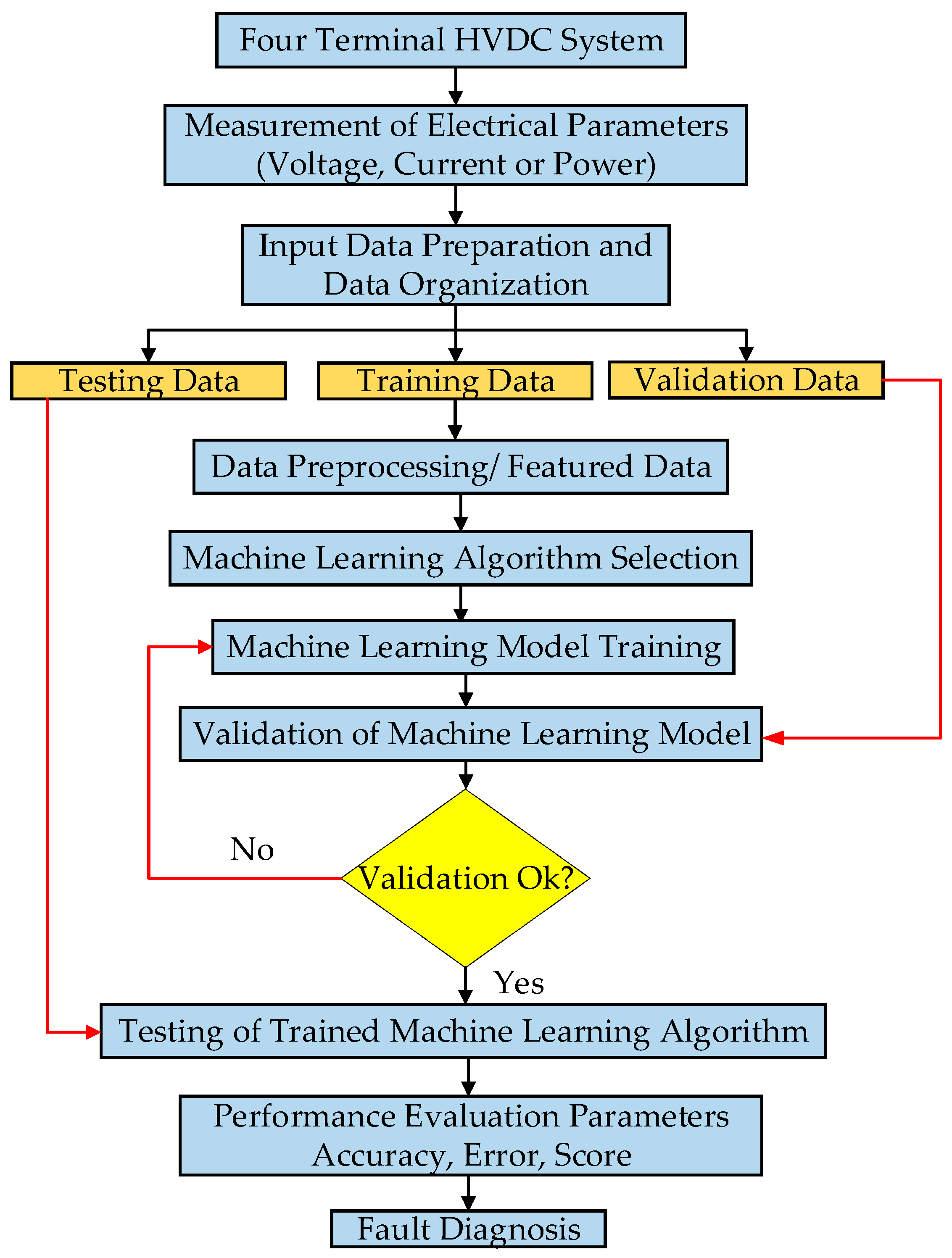
3. Proposed Methodology for Fault Diagnosis
3.1. Evaluation of Trained Algorithm
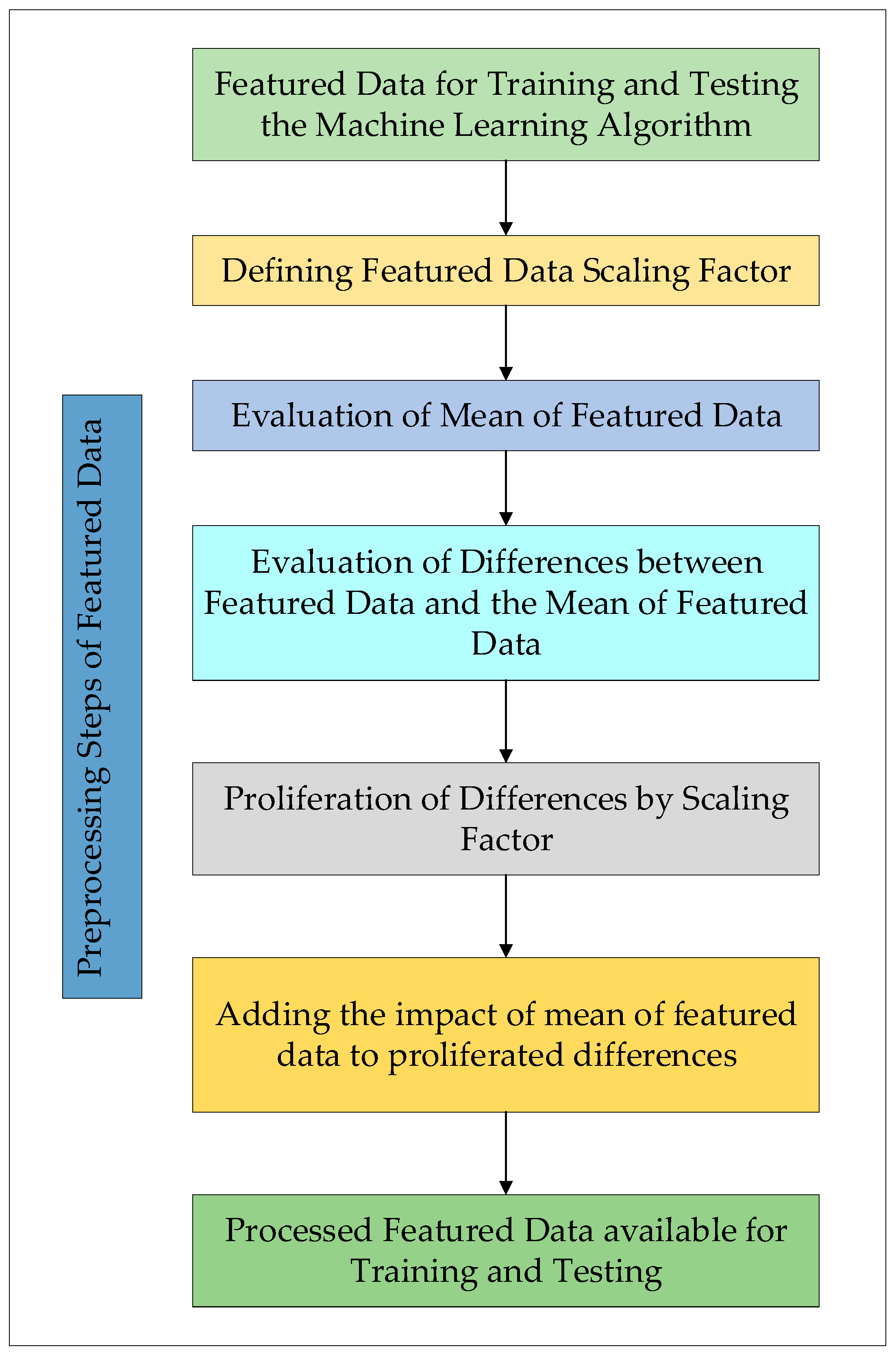
3.2. Proposed Modification for Accuracy Improvement
4. Simulation Results and Analysis
4.1. Fault Current Based Scenarios
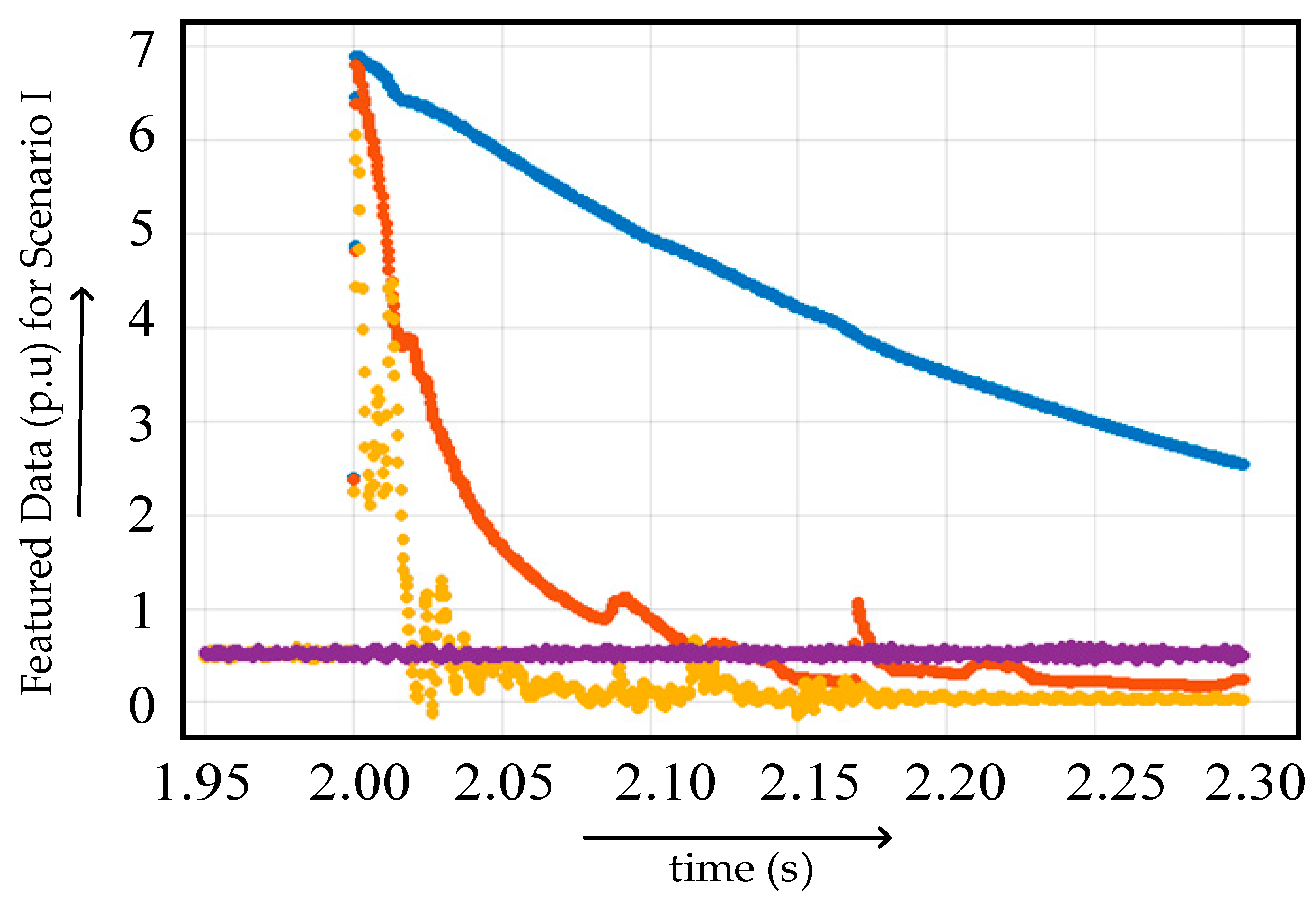
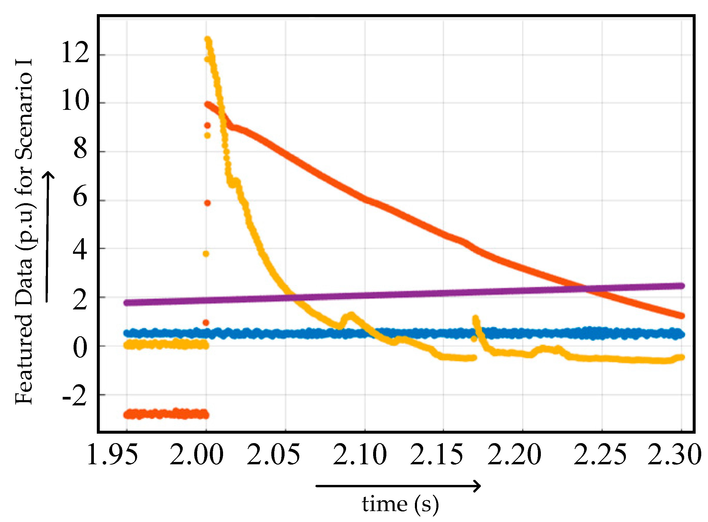
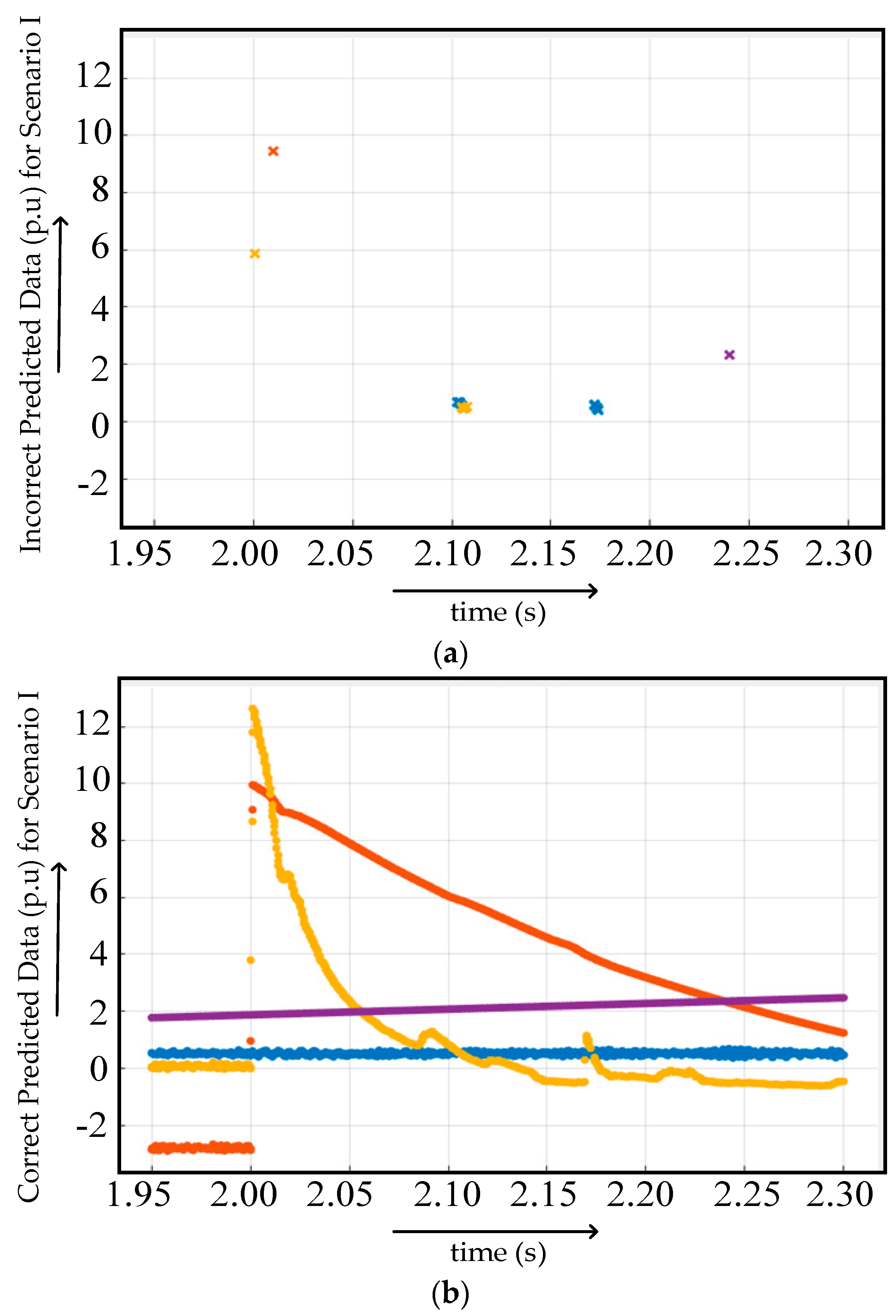
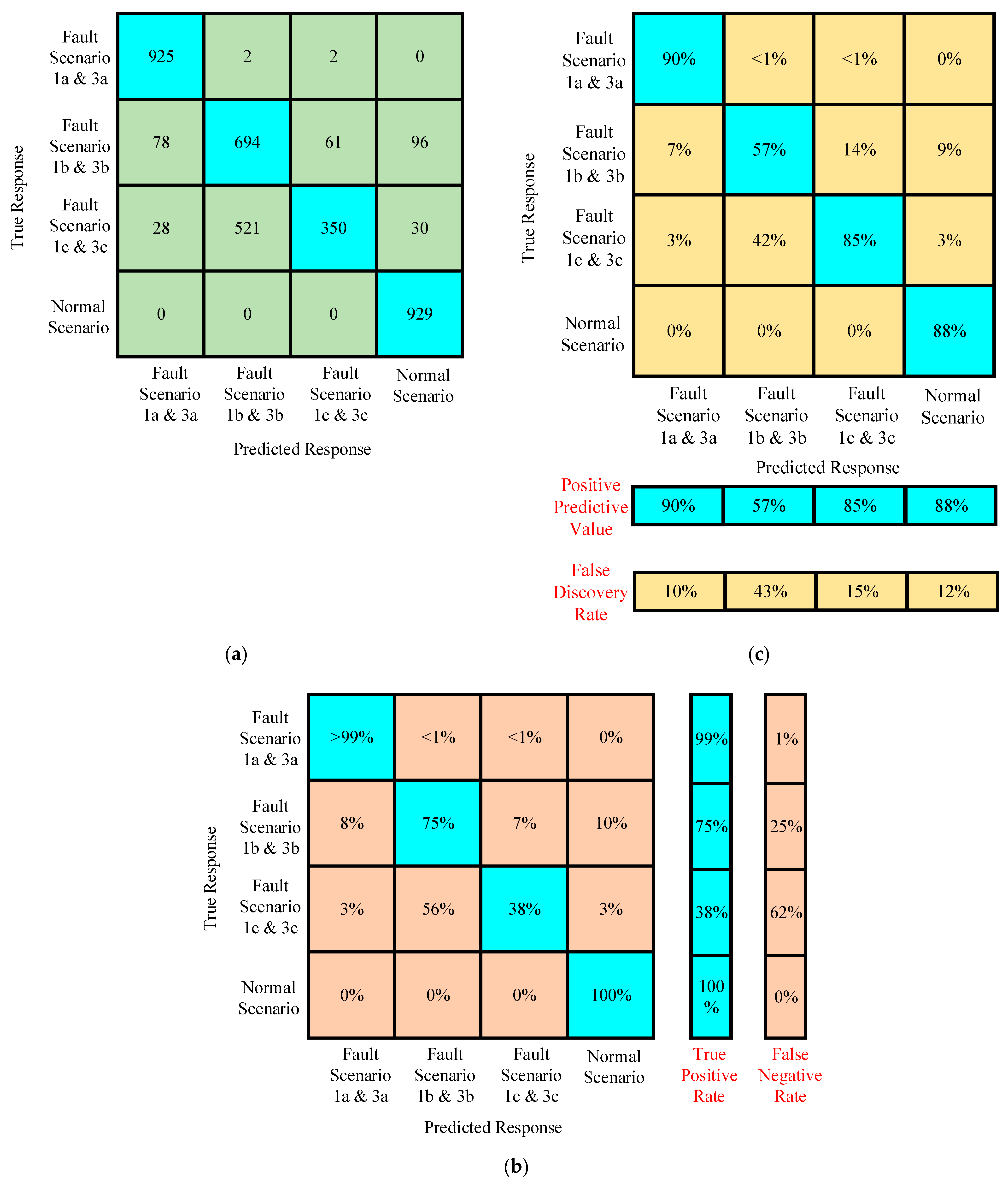
4.1.1. Scenario 1
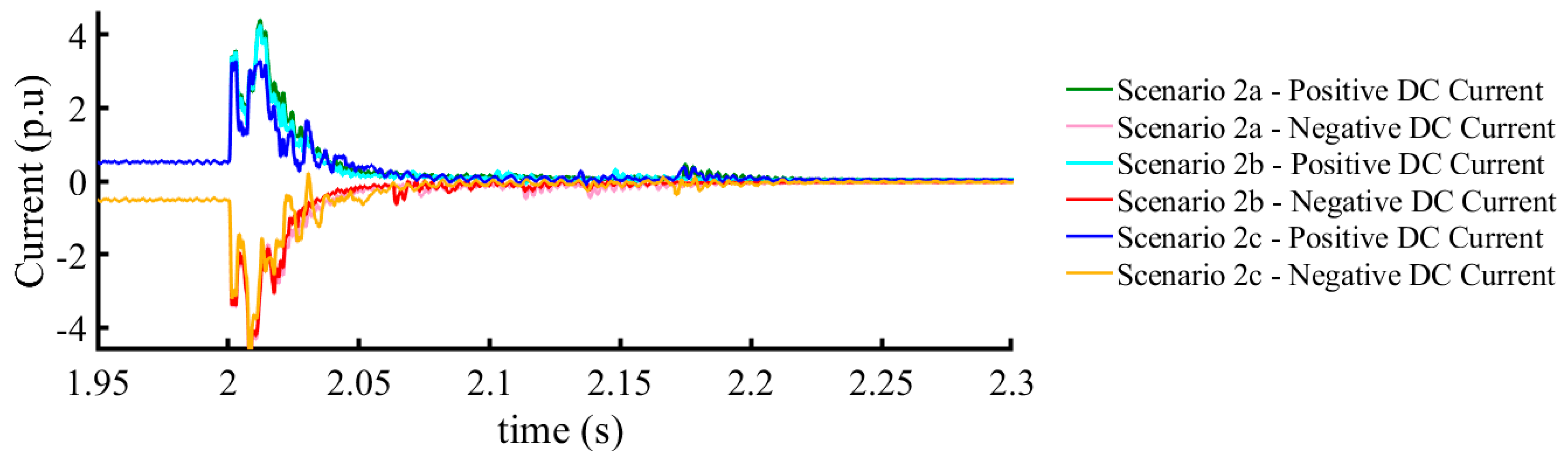
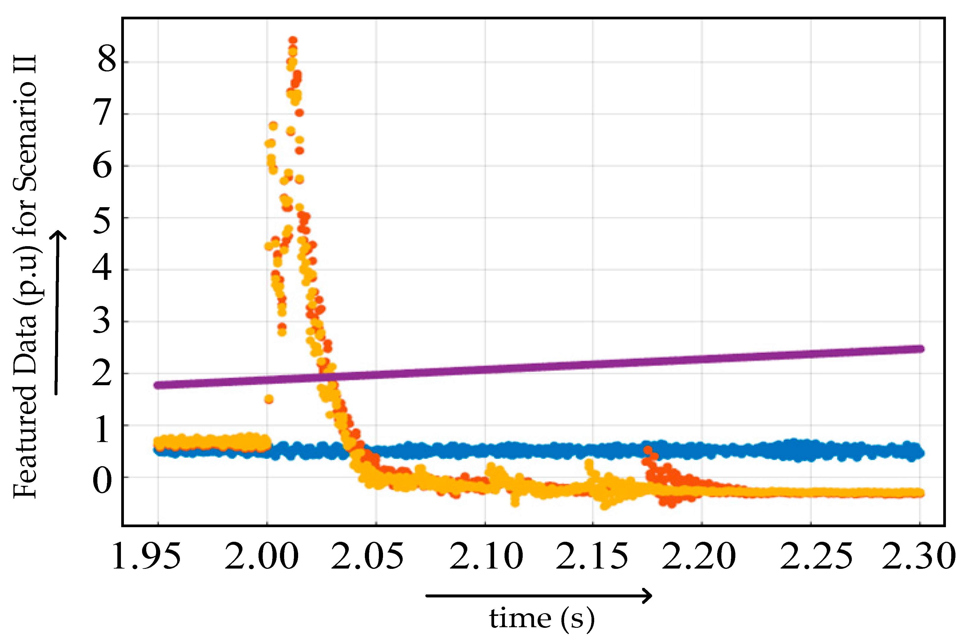
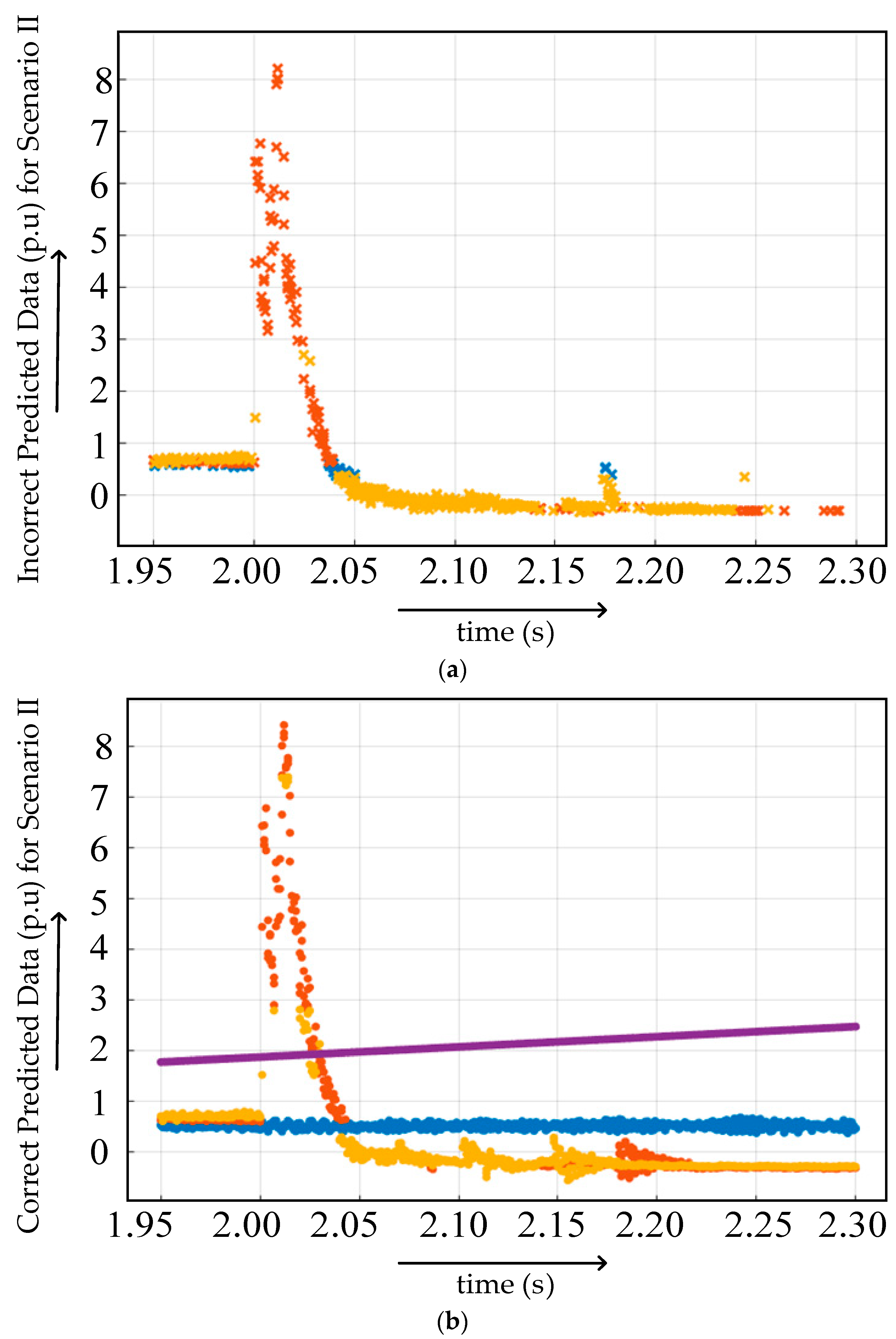
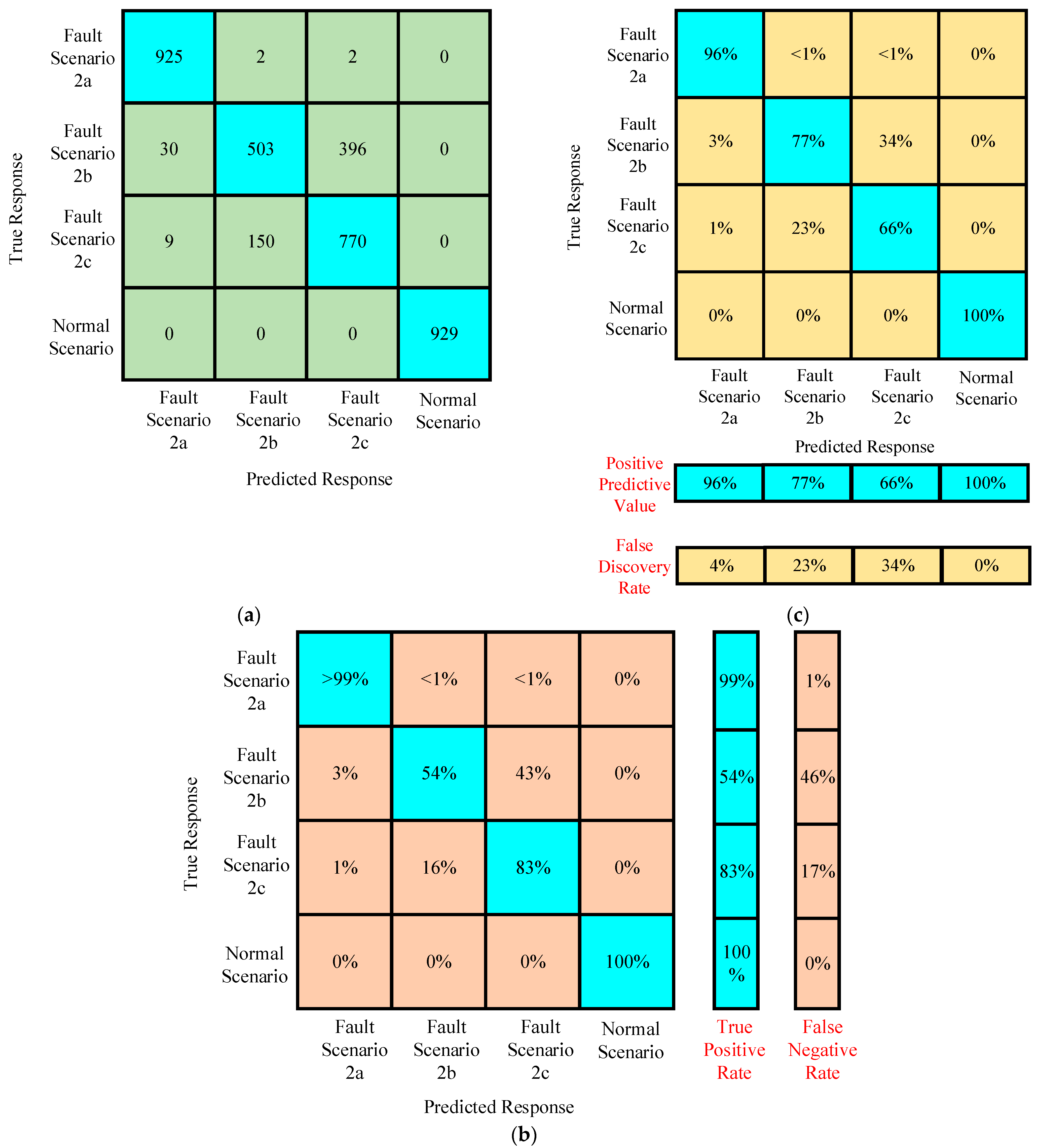
4.1.2. Scenario 2
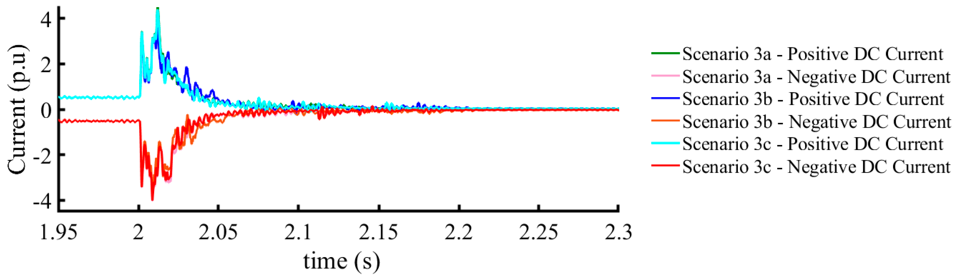
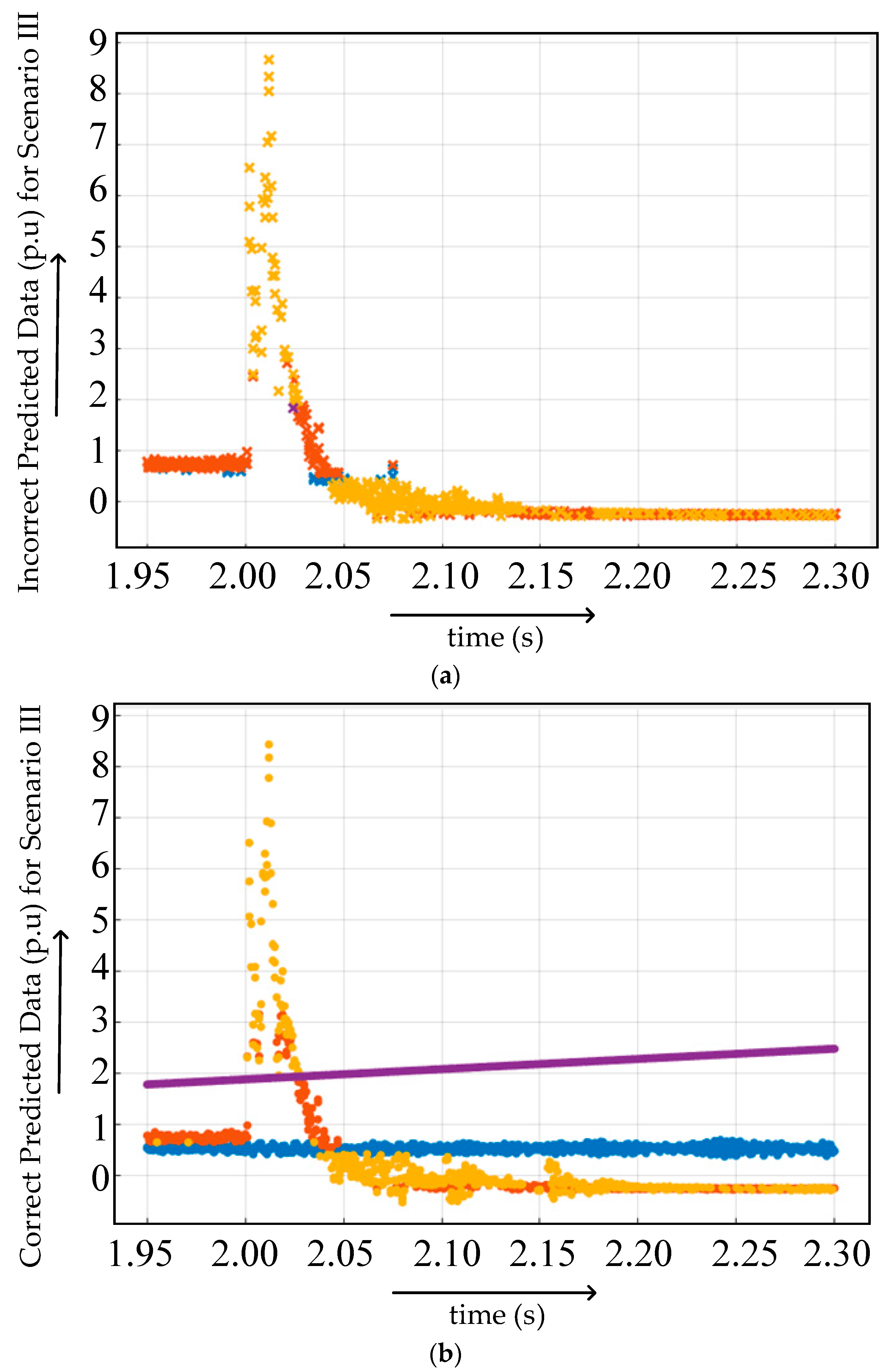
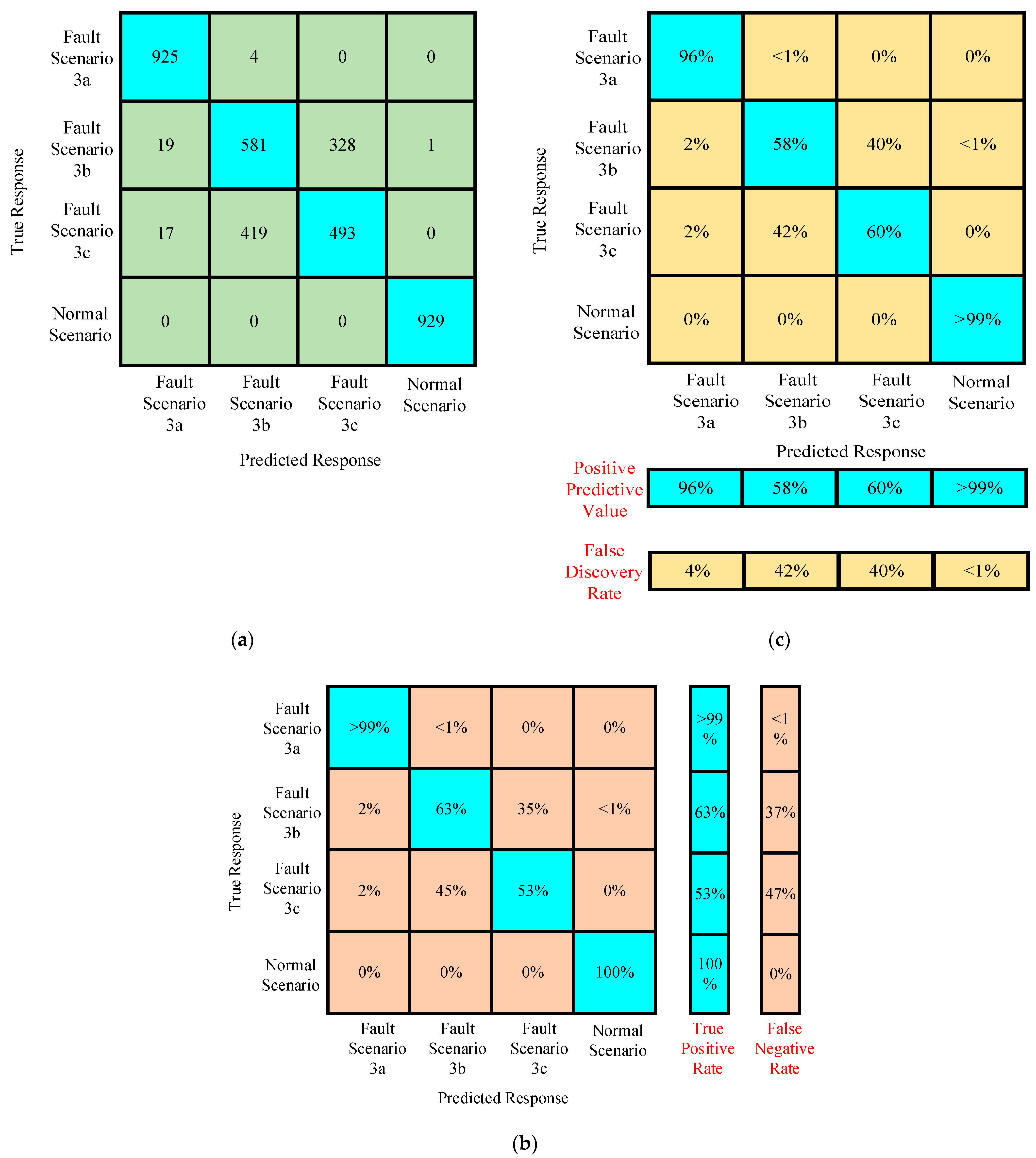
4.1.3. Scenario 3
4.2. Featured Data-Based Simulation Cases
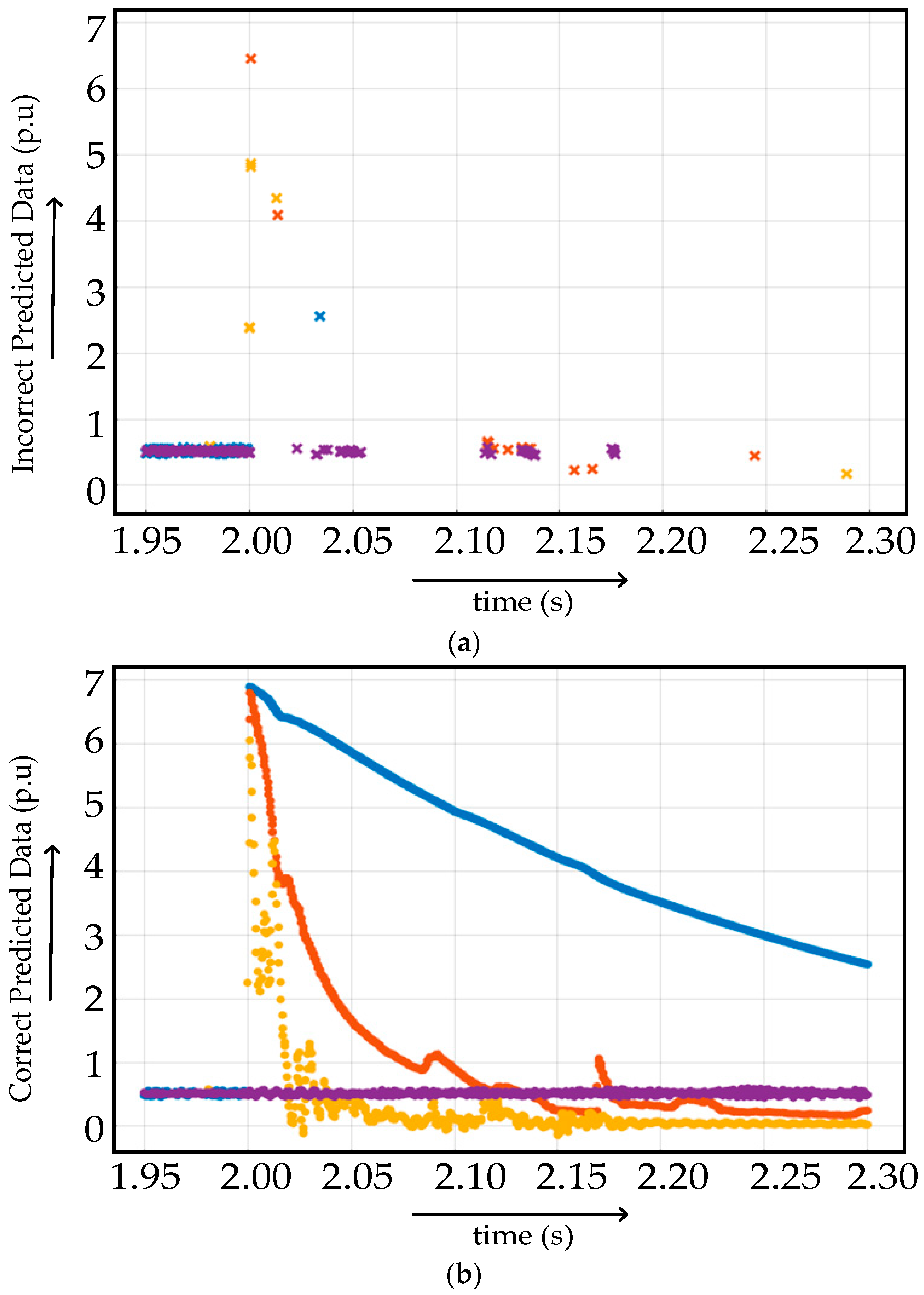
4.2.1. Case I
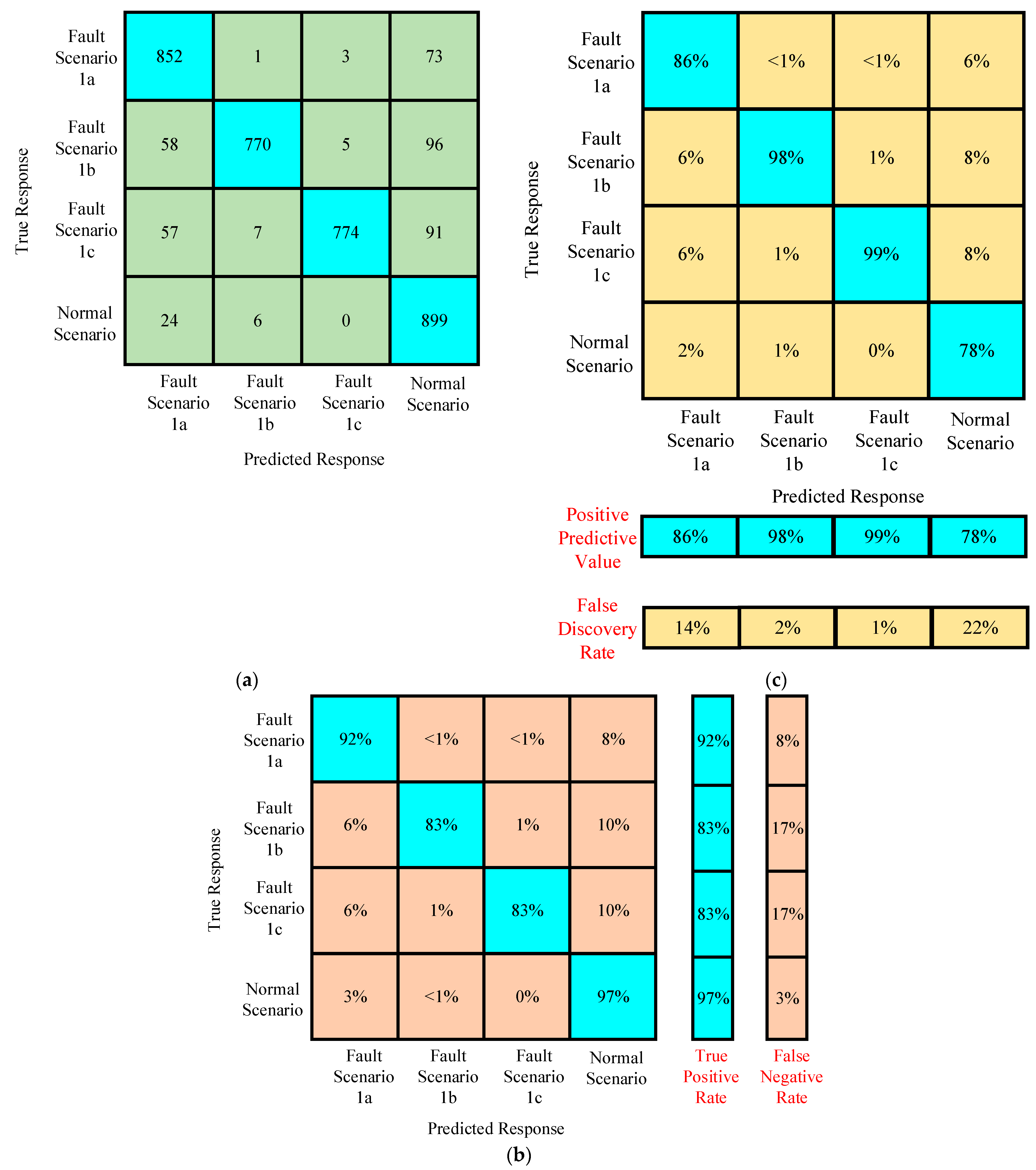
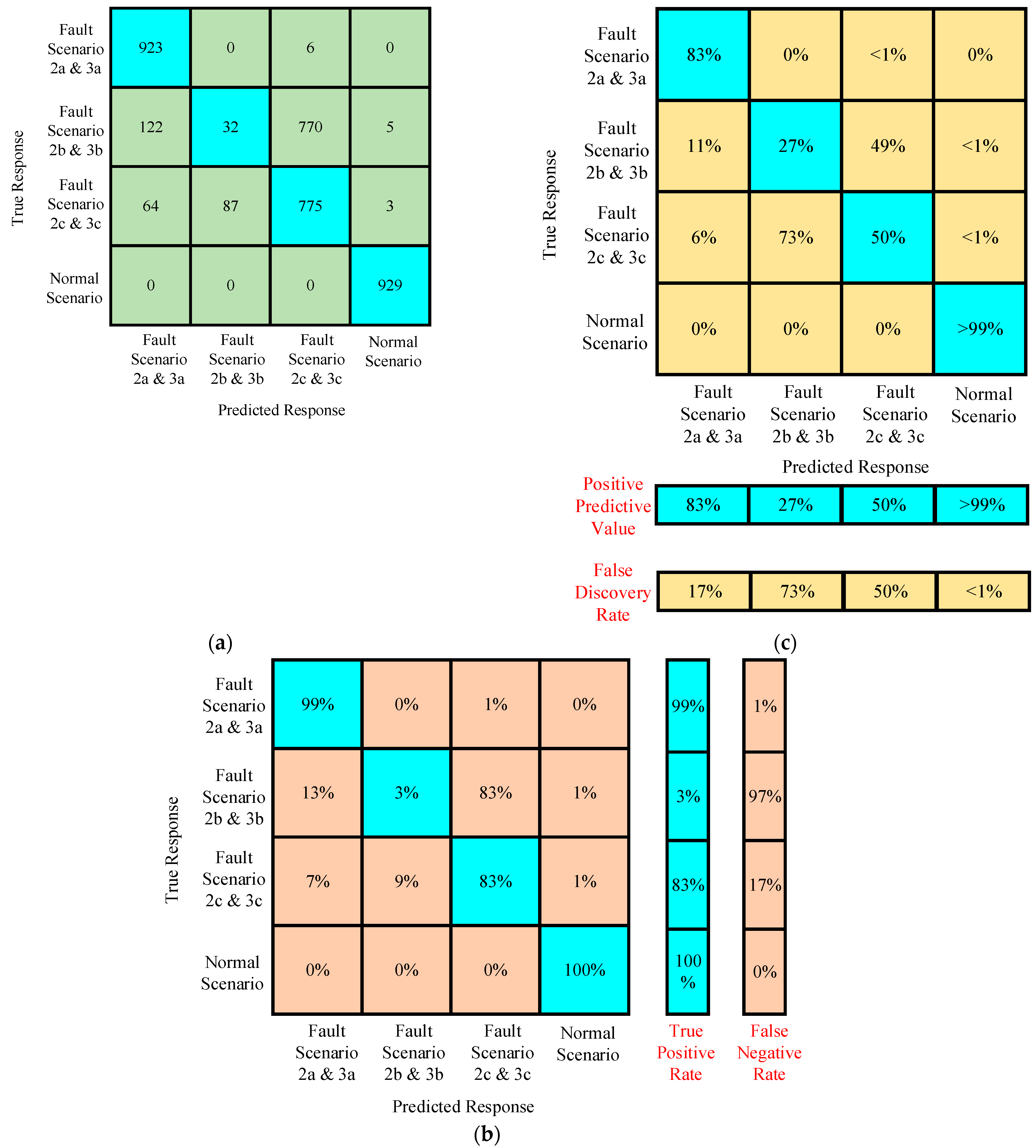
Confusion Matrices for Training Under Case I
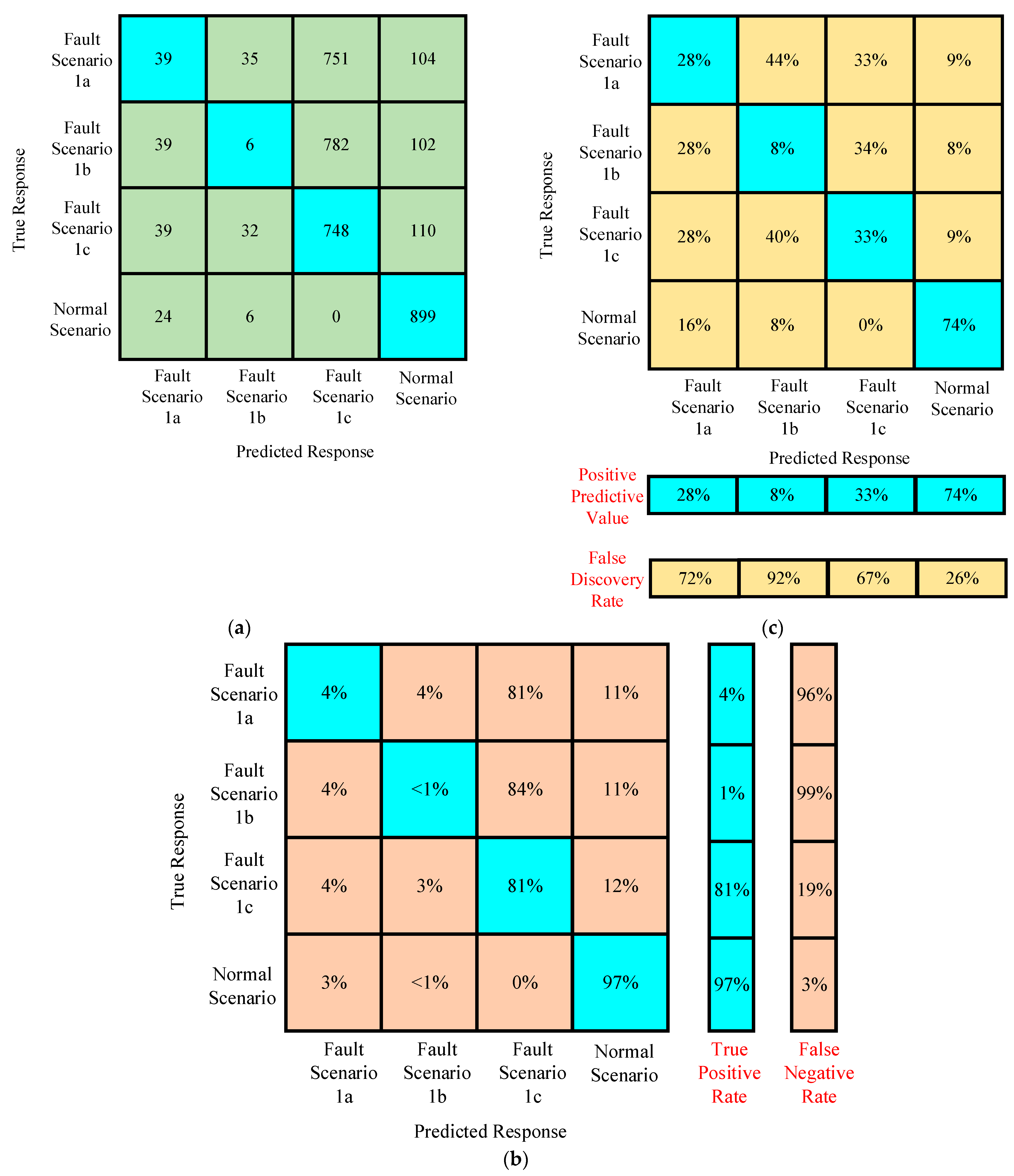
Confusion Matrices for Testing Under Case I
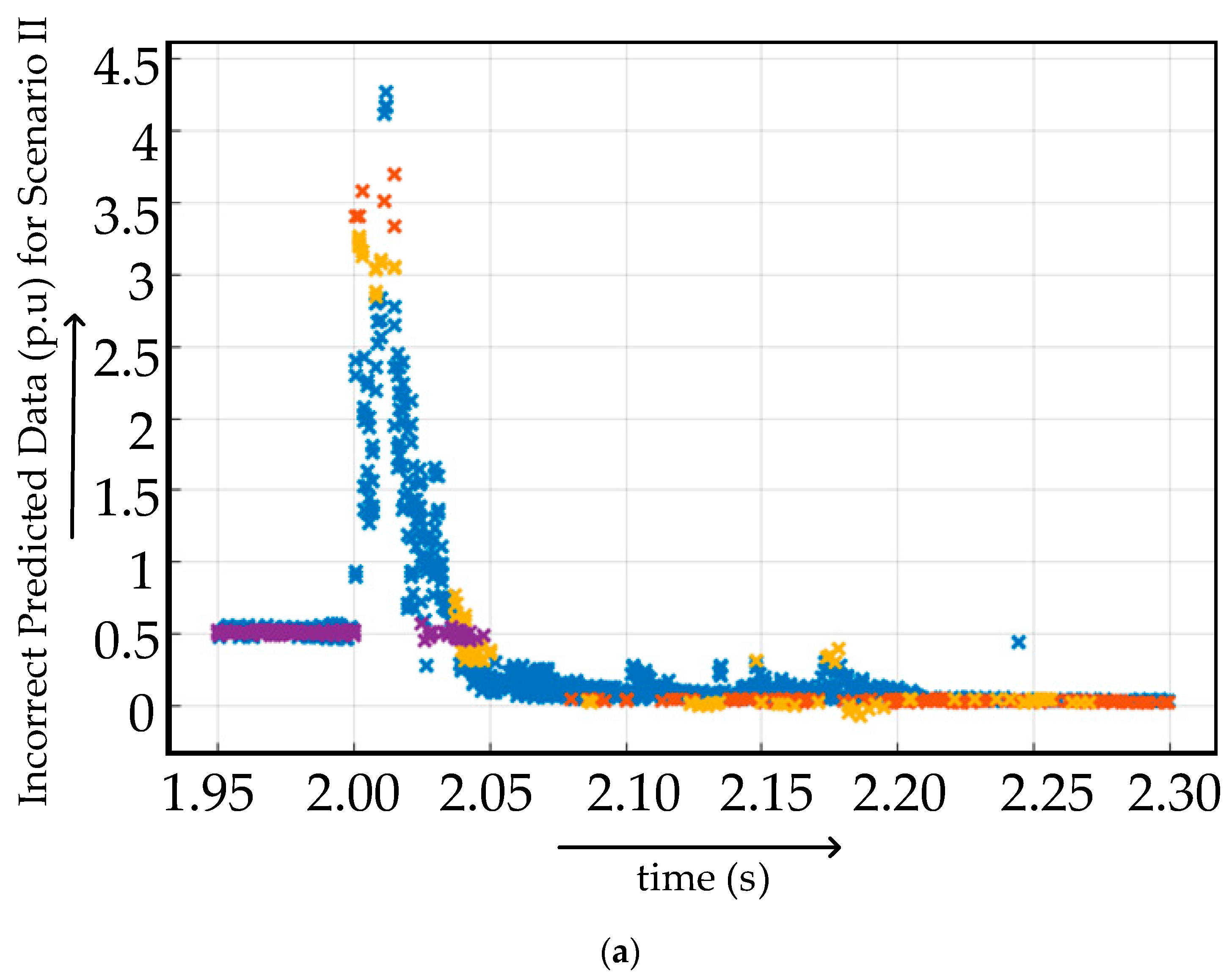
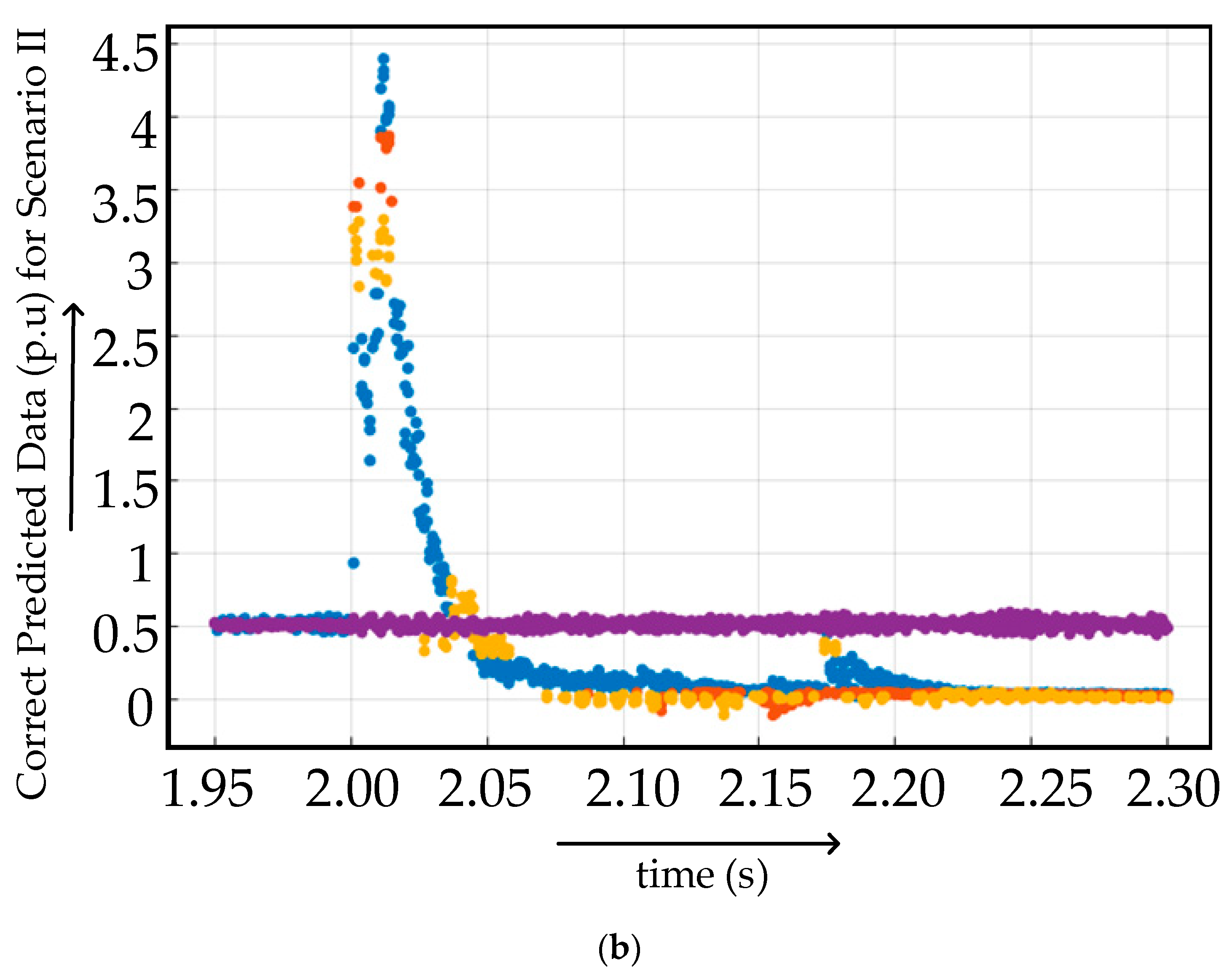
4.2.2. Case II
Confusion Matrices for Training Under Case II
Confusion Matrices for Testing Under Case II
4.2.3. Case III
Confusion Matrices for Training Under Case III
Confusion Matrices for Testing Under Case III
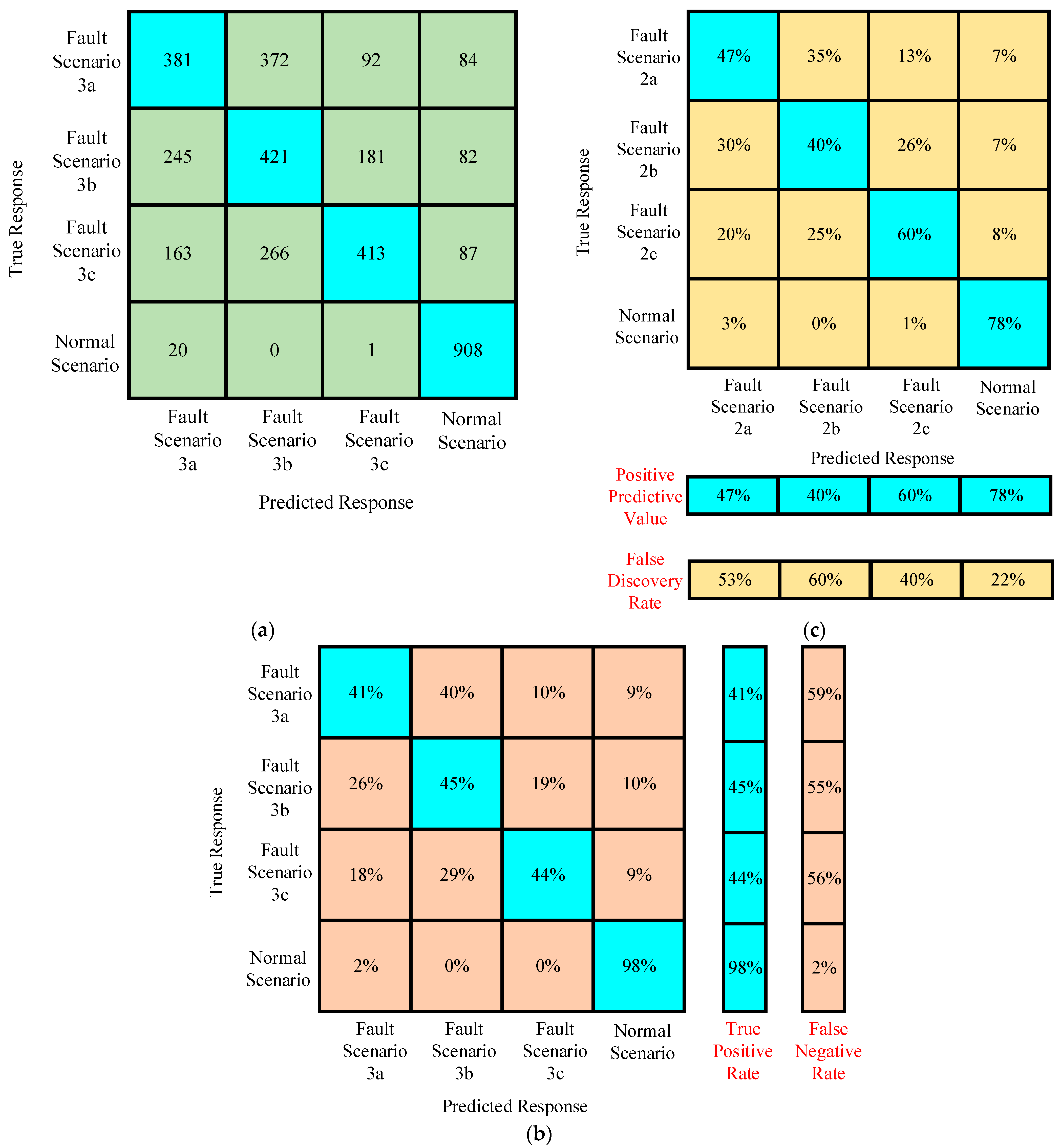
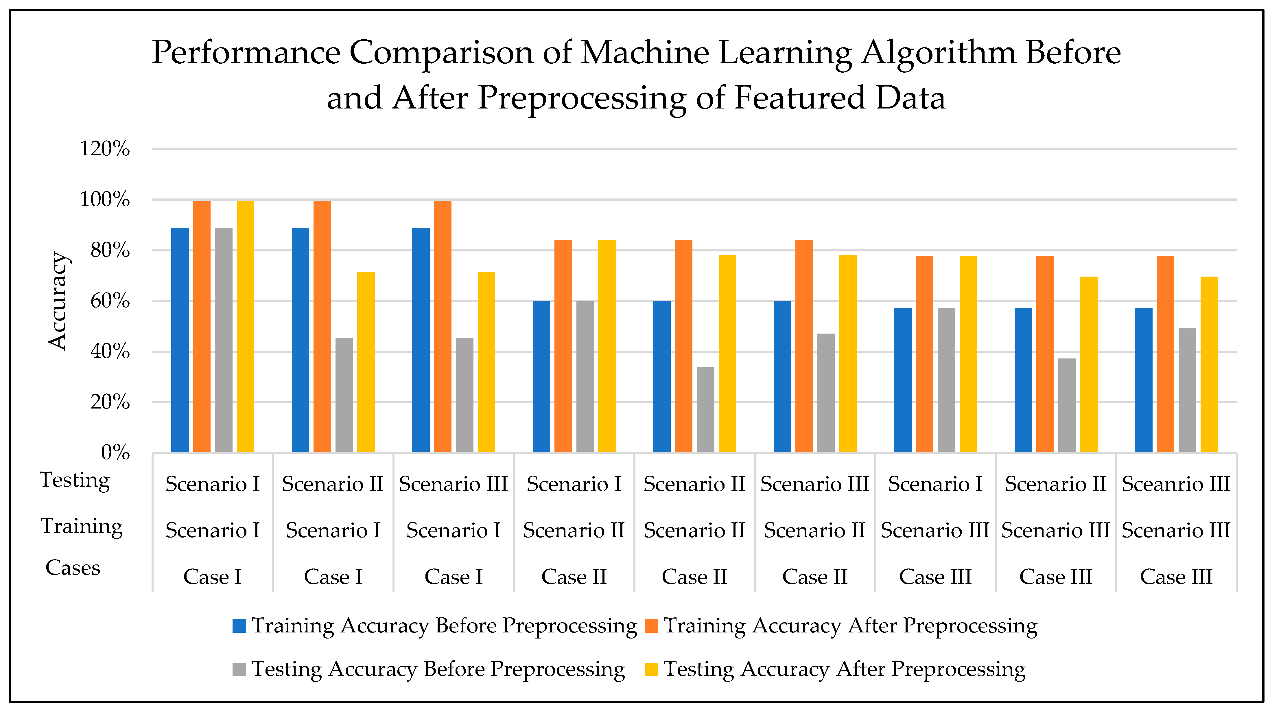
4.3. Accuracy Improvement-Based Simulation Cases
4.3.1. Case I
Confusion Matrices for Training of Algorithm Under Preprocessed Featured Data of Case I
Confusion Matrices for Testing of Algorithm Under Preprocessed Featured Data of Case I
- The accuracy of testing the trained algorithm with the data having the same features used for training was around 99.5%.
- The accuracy of testing the trained algorithm with the new data improved to 26.03%.
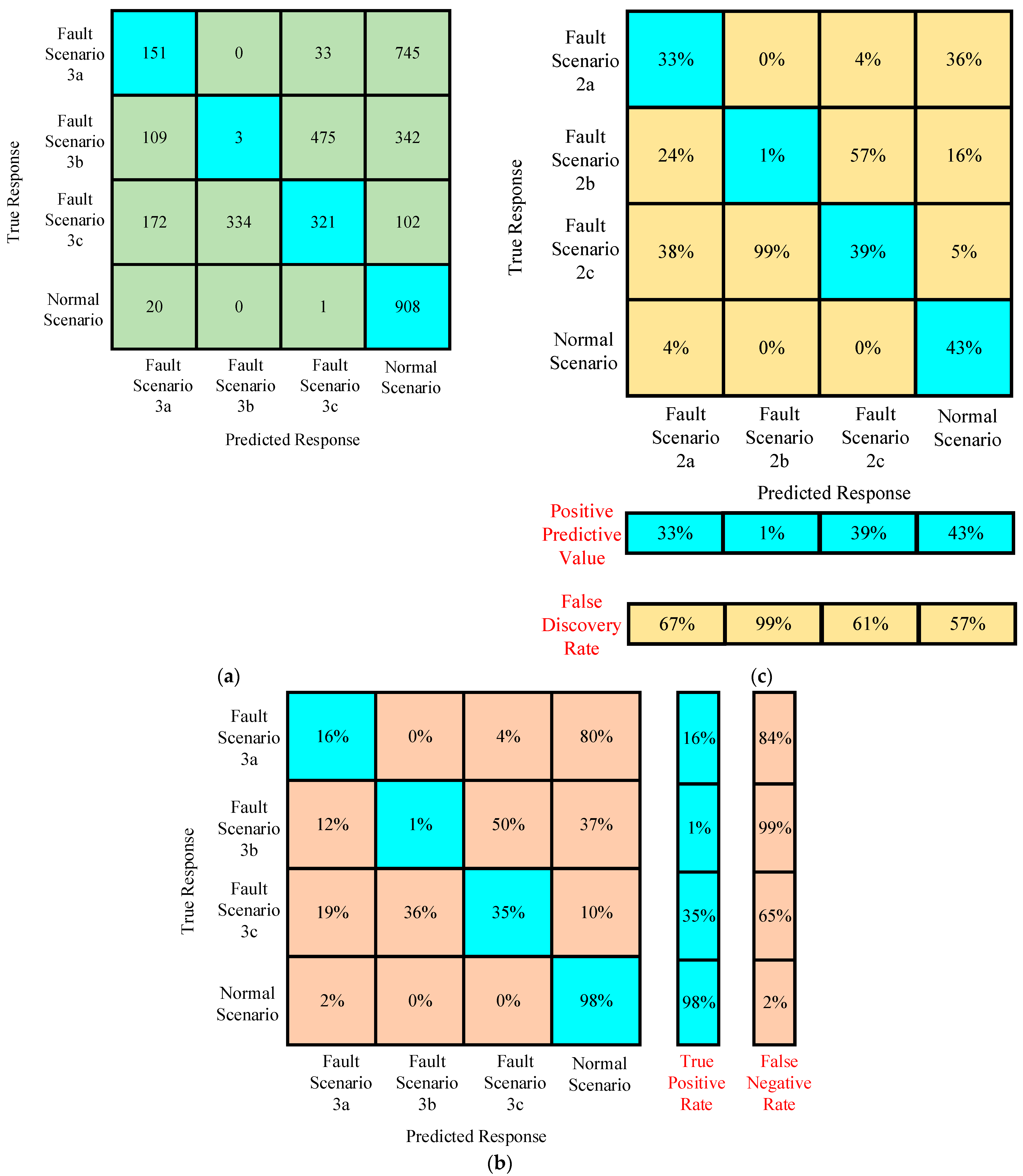
4.3.2. Case II
Confusion Matrices for Training of Algorithm Under Preprocessed Featured Data of Case II
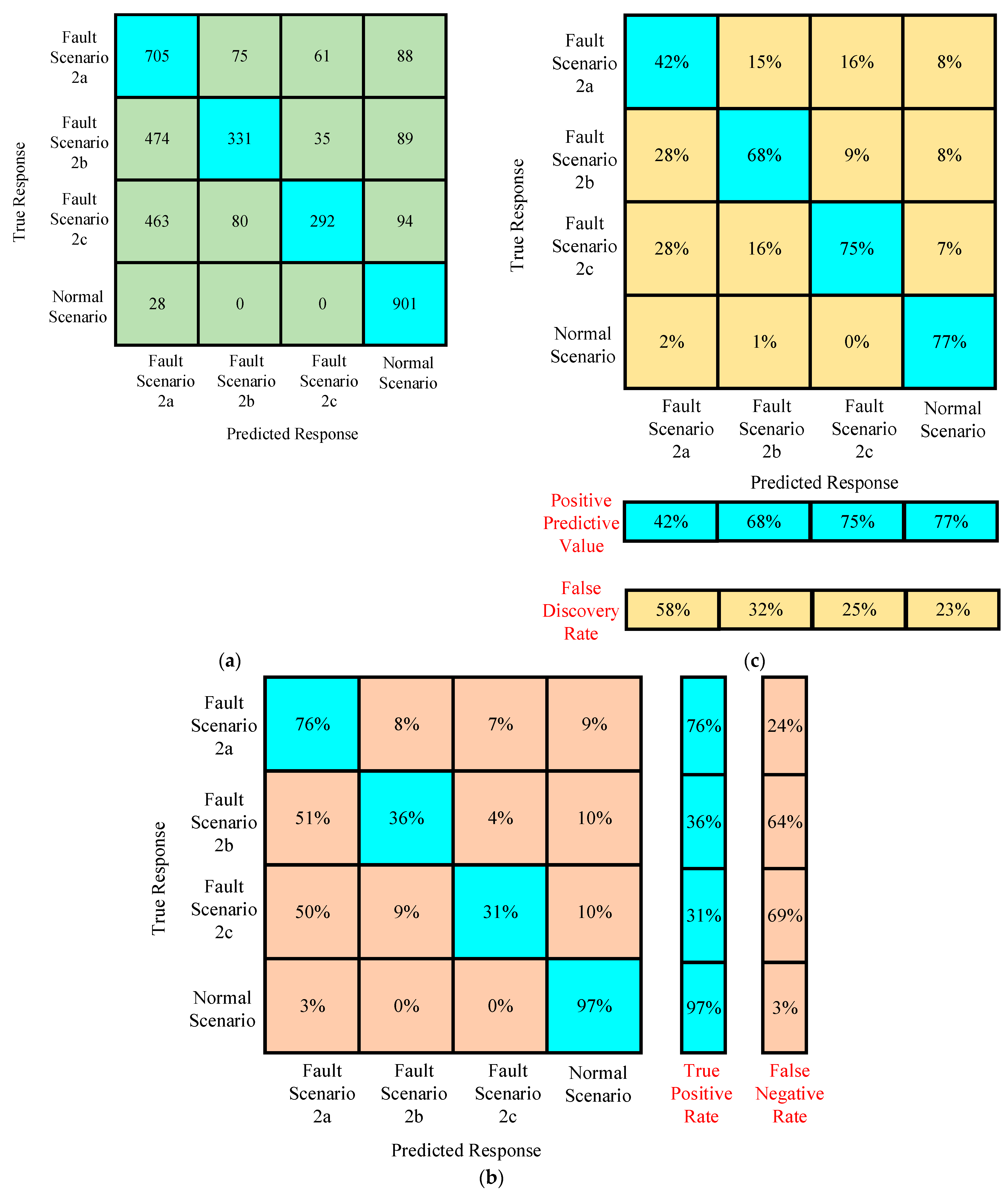
Confusion Matrices for Testing Algorithm Under Preprocessed Featured Data of Case II
- 3.
- The accuracy of testing the trained algorithm with the data having the same features used for training is around 84.1%. Hence, preprocessing of featured data increases the accuracy by up to 24.1%.
- 4.
- The accuracy of testing the trained algorithm with the new data is improved up to an average of 37.52%.
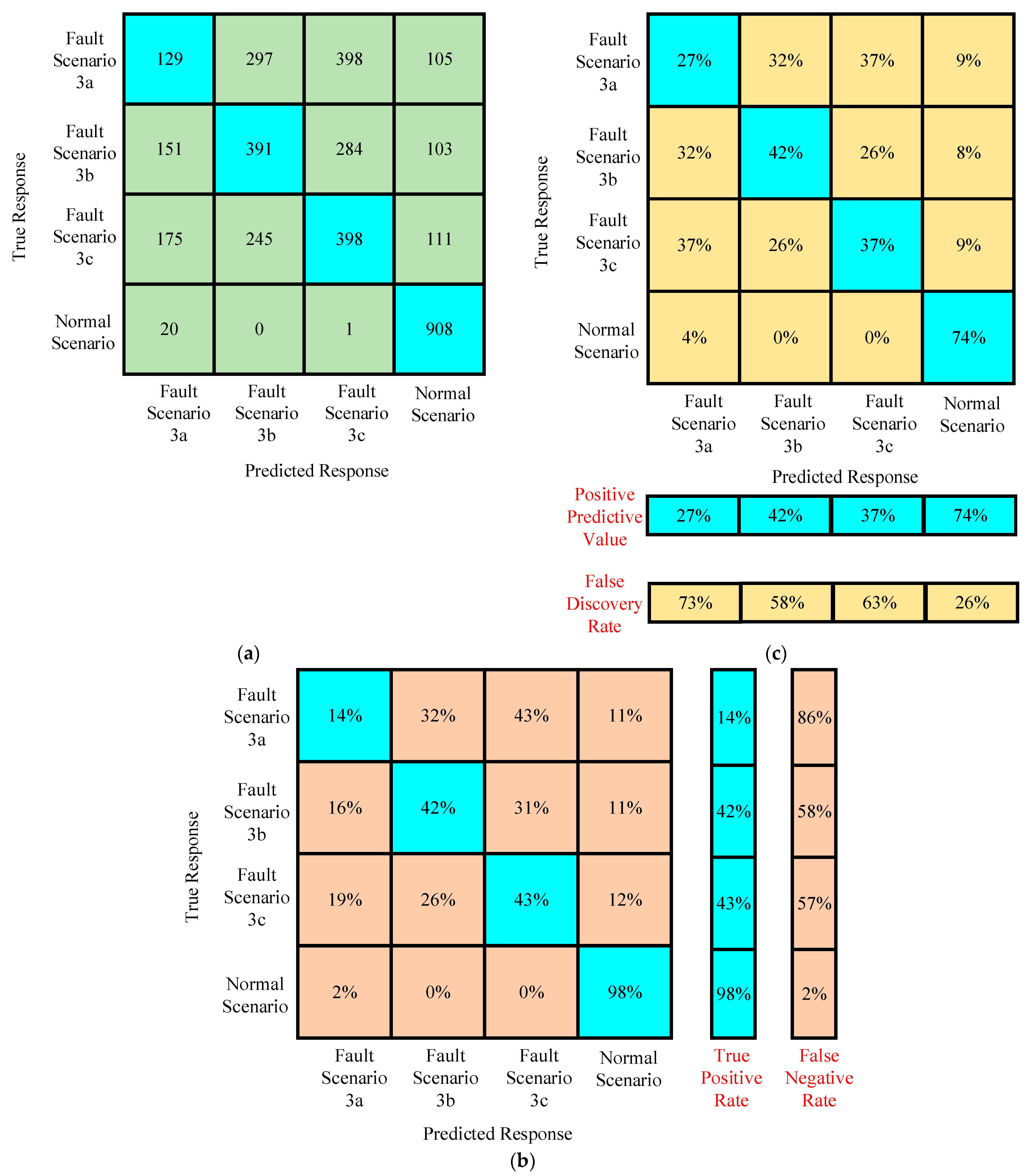
4.3.3. Case III
Confusion Matrices for Training Algorithm Under Preprocessed Featured Data of Case III
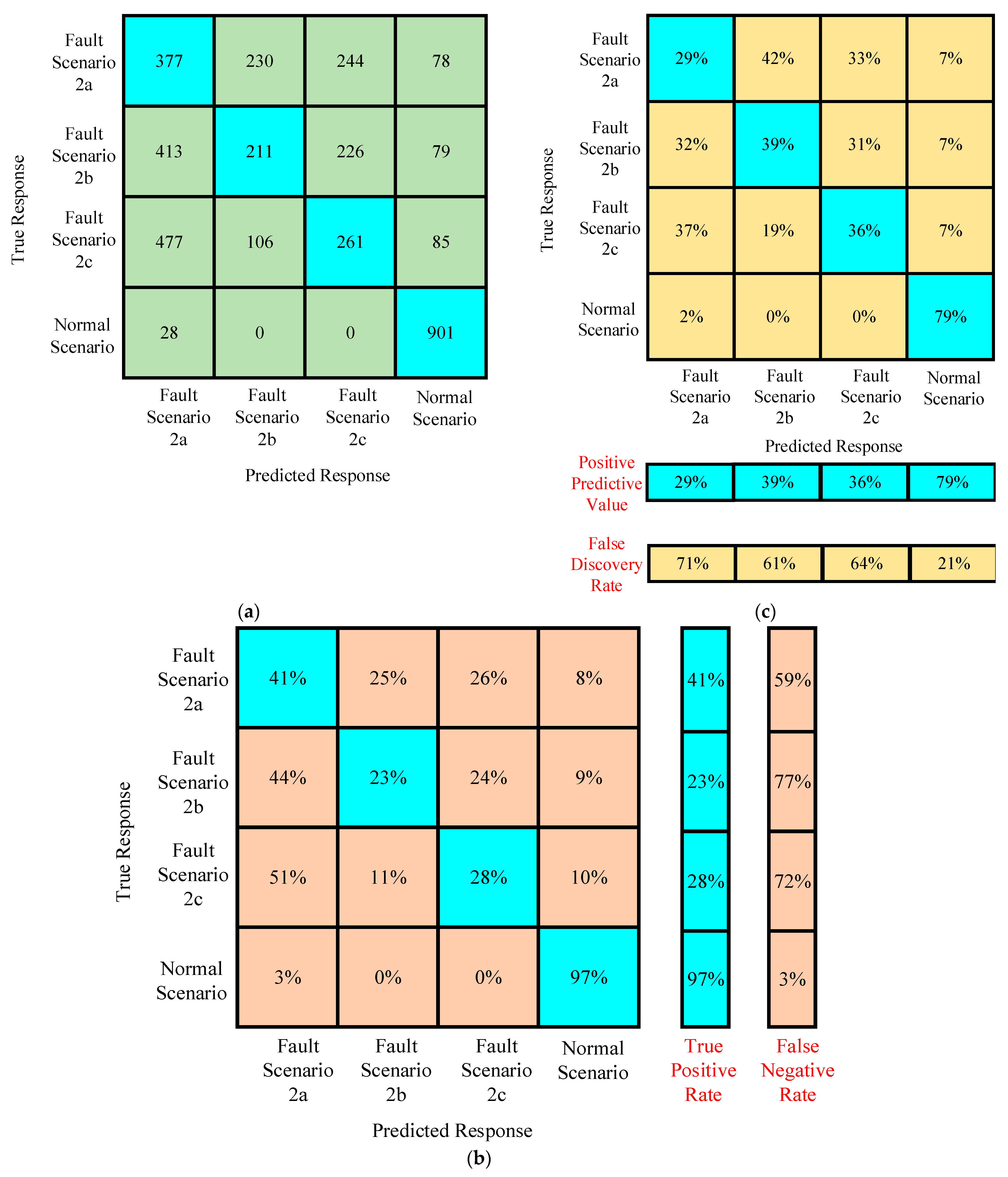
Confusion Matrices for Testing Algorithm Under Preprocessed Featured Data of Case III
4.4. Research Limitations
4.5. Annotations of Research for Protection
- The accuracy of fault classification is improved significantly without adding challenging computational overheads.
- Preprocessing based on the simple computation of mean and differences has aided Gini’s index of diversity-based classification remarkably.
- Table 7 indicates that scenarios with high values of fault and ground resistances in the test system are associated with a significant improvement in accuracy.
- Less complexity offers a relatively better classification of faults based on location with easy interpretation.
4.6. Comparison with Existing Machine Learning Techniques
4.7. Computational Complexity Analysis of Proposed Technique
4.8. Real-Time Implementation Consideration of Proposed Technique
5. Conclusions
Possible Future Directions
- Pole-to-pole faults can be made part of the research under different fault and ground resistances and with a medium tree-based machine learning algorithm.
- The hybrid approach of machine learning techniques for fault diagnosis can be developed in which online fault diagnosis can be performed with the simplified machine learning algorithm, and offline in-depth fault studies can be performed with the advanced and computationally extensive machine learning algorithms.
- More methods of preprocessing can be explored so that the accuracy can be retained at higher values with the higher values of fault and ground resistances.
- Internal and external faults based on zones and protection can be analyzed for the multiterminal system. Fault diagnosis can be carried out with the medium tree-based machine algorithm which has the wonderful feature of avoiding overfitting and outliers.
- Relay coordination setup can be simulated with the medium tree-based machine learning algorithm because of its rapid response with less data and computational time.
Funding
Data Availability Statement
Acknowledgments
Conflicts of Interest
References
- Sneath, J.; Rajapakse, A.D. Fault Detection and Interruption in an Earthed HVDC Grid Using ROCOV and Hybrid DC Breakers. IEEE Trans. Power Deliv. 2016, 31, 973–981. [Google Scholar] [CrossRef]
- Wang, L.; Liu, H.; Dai, L.; Liu, Y. Novel Method for Identifying Fault Location of Mixed Lines. Energies 2018, 11, 1529. [Google Scholar] [CrossRef]
- Farshad, M.; Sadeh, J. A Novel Fault-Location Method for HVDC Transmission Lines Based on Similarity Measure of Voltage Signals. IEEE Trans. Power Deliv. 2013, 28, 2483–2490. [Google Scholar] [CrossRef]
- Muzzammel, R. Traveling Waves-Based Method for Fault Estimation in HVDC Transmission System. Energies 2019, 12, 3614. [Google Scholar] [CrossRef]
- Muzzammel, R.; Raza, A.; Hussain, M.R.; Abbas, G.; Ahmed, I.; Qayyum, M.; Rasool, M.A.; Khaleel, M.A. MT–HVdc Systems Fault Classification and Location Methods Based on Traveling and Non-Traveling Waves—A Comprehensive Review. Appl. Sci. 2019, 9, 4760. [Google Scholar] [CrossRef]
- Yang, J.; Fletcher, J.E.; O’Reilly, J. Short-Circuit and Ground Fault Analyses and Location in VSC-Based DC Network Cables. IEEE Trans. Ind. Electron. 2012, 59, 3827–3837. [Google Scholar] [CrossRef]
- Ye, X.; Lan, S.; Xiao, S.; Yuan, Y. Single Pole-to-Ground Fault Location Method for MMC-HVDC System Using Wavelet Decomposition and DBN. IEEJ Trans. Electr. Electron. Eng. 2021, 16, 238–247. [Google Scholar] [CrossRef]
- Swetapadma, A.; Agarwal, S.; Chakrabarti, S.; Chakrabarti, S.; El-Shahat, A.; Abdelaziz, A.Y. Locating Faults in Thyristor-Based LCC-HVDC Transmission Lines Using Single End Measurements and Boosting Ensemble. Electronics 2022, 11, 186. [Google Scholar] [CrossRef]
- Ashouri, M.; da Silva, F.F.; Bak, C.L. On the Application of Modal Transient Analysis for Online Fault Localization in HVDC Cable Bundles. IEEE Trans. Power Deliv. 2020, 35, 1365–1378. [Google Scholar] [CrossRef]
- Zhai, S.; Cui, Y.; Li, F.; Wang, R.; Su, W.; Tang, H. VSC-HVDC Fault Location Method Based on Effective Feature and Depth Belief Network. J. Phys. Conf. Ser. 2022, 2409, 012027. [Google Scholar] [CrossRef]
- Chen, Q.; Wu, J.; Li, Q.; Gao, X.; Yu, R.; Guo, J.; Peng, G.; Yang, B. Long Short-Term Memory Network-Based HVDC Systems Fault Diagnosis under Knowledge Graph. Electronics 2023, 12, 2242. [Google Scholar] [CrossRef]
- Li, K.-Q.; Yin, Z.-Y.; Zhang, N.; Liu, Y. A Data-Driven Method to Model Stress-Strain Behaviour of Frozen Soil Considering Uncertainty. Cold Reg. Sci. Technol. 2023, 213, 103906. [Google Scholar] [CrossRef]
- Angra, S.; Ahuja, S. Machine Learning and Its Applications: A Review. In Proceedings of the 2017 International Conference on Big Data Analytics and Computational Intelligence (ICBDAC), Chirala, Andhra Pradesh, India, 23–25 March 2017; IEEE: Piscataway, NJ, USA; pp. 57–60. [Google Scholar]
- Li, L.; Wu, Y.; Ou, Y.; Li, Q.; Zhou, Y.; Chen, D. Research on Machine Learning Algorithms and Feature Extraction for Time Series. In Proceedings of the 2017 IEEE 28th Annual International Symposium on Personal, Indoor, and Mobile Radio Communications (PIMRC), Montreal, QC, Canada, 8–13 October 2017; IEEE: Piscataway, NJ, USA; pp. 1–5. [Google Scholar]
- Kumar, Y.; Kaur, K.; Singh, G. Machine Learning Aspects and Its Applications Towards Different Research Areas. In Proceedings of the 2020 International Conference on Computation, Automation and Knowledge Management (ICCAKM): Dubai, United Arab Emirates, 9–10 January 2020; IEEE: Piscataway, NJ, USA; pp. 150–156. [Google Scholar]
- Li, K.; Horton, R.; He, H. Application of Machine Learning Algorithms to Model Soil Thermal Diffusivity. Int. Commun. Heat Mass Transf. 2023, 149, 107092. [Google Scholar] [CrossRef]
- Luo, G.; Yao, C.; Tan, Y.; Liu, Y. Transient Signal Identification of HVDC Transmission Lines Based on Wavelet Entropy and SVM. J. Eng. 2019, 2019, 2414–2419. [Google Scholar] [CrossRef]
- Chen, M.-J.; Lan, S.; Chen, D.-Y. Machine Learning Based One-Terminal Fault Areas Detection in HVDC Transmission System. In Proceedings of the 2018 8th International Conference on Power and Energy Systems (ICPES), Colombo, Sri Lanka, 21–22 December 2018; IEEE: Piscataway, NJ, USA; pp. 278–282. [Google Scholar]
- Lan, S.; Chen, M.-J.; Chen, D.-Y. A Novel HVDC Double-Terminal Non-Synchronous Fault Location Method Based on Convolutional Neural Network. IEEE Trans. Power Deliv. 2019, 34, 848–857. [Google Scholar] [CrossRef]
- Hossam-Eldin, A.; Lotfy, A.; Elgamal, M.; Ebeed, M. Artificial Intelligence-based Short-circuit Fault Identifier for MT-HVDC Systems. IET Gener. Transm. Amp; Distrib. 2018, 12, 2436–2443. [Google Scholar] [CrossRef]
- Unal, F.; Ekici, S. A Fault Location Technique for HVDC Transmission Lines Using Extreme Learning Machines. In Proceedings of the 2017 5th International Istanbul Smart Grid and Cities Congress and Fair (ICSG), Istanbul, Turkey, 19–21 April 2017; IEEE: Piscataway, NJ, USA; pp. 125–129. [Google Scholar]
- Hossam-Eldin, A.; Lotfy, A.; Elgamal, M.; Ebeed, M. Combined Traveling Wave and Fuzzy Logic Based Fault Location in Multi-Terminal HVDC Systems. In Proceedings of the 2016 IEEE 16th International Conference on Environment and Electrical Engineering (EEEIC), Florence, Italy, 7–10 June 2016; IEEE: Piscataway, NJ, USA; pp. 1–6. [Google Scholar]
- Dudve, R.; Goad, S. A Review on Automated Techniques for Fault Location in HVDC Systems. IJSREM 2022, 6, 1–5. [Google Scholar] [CrossRef]
- He, Z.; Liao, K.; Li, X.; Lin, S.; Yang, J.; Mai, R. Natural Frequency-Based Line Fault Location in HVDC Lines. IEEE Trans. Power Deliv. 2014, 29, 851–859. [Google Scholar] [CrossRef]
- Muzzammel, R. Machine Learning Based Fault Diagnosis in HVDC Transmission Lines. In Intelligent Technologies and Applications; Bajwa, I.S., Kamareddine, F., Costa, A., Eds.; Communications in Computer and Information Science; Springer: Singapore, 2019; Volume 932, pp. 496–510. ISBN 978-981-13-6051-0. [Google Scholar]
- Luo, G.; Yao, C.; Liu, Y.; Tan, Y.; He, J.; Wang, K. Stacked Auto-Encoder Based Fault Location in VSC-HVDC. IEEE Access 2018, 6, 33216–33224. [Google Scholar] [CrossRef]
- Razzaghi, R.; Paolone, M.; Rachidi, F.; Descloux, J.; Raison, B.; Retiere, N. Fault Location in Multi-Terminal HVDC Networks Based on Electromagnetic Time Reversal with Limited Time Reversal Window. In Proceedings of the 2014 Power Systems Computation Conference, Wroclaw, Poland, 18–22 August 2014; IEEE: Piscataway, NJ, USA; pp. 1–7. [Google Scholar]
- Triveno, J.P.; Dardengo, V.P.; De Almeida, M.C. An Approach to Fault Location in HVDC Lines Using Mathematical Morphology. In Proceedings of the 2015 IEEE Power & Energy Society General Meeting, Denver, CO, USA, 26–30 July 2015; IEEE: Piscataway, NJ, USA; pp. 1–5. [Google Scholar]
- Yi-ning, Z.; Yong-hao, L.; Min, X.; Ze-xiang, C. A Novel Algorithm for HVDC Line Fault Location Based on Variant Travelling Wave Speed. In Proceedings of the 2011 4th International Conference on Electric Utility Deregulation and Restructuring and Power Technologies (DRPT), Weihai, China, 6–9 July 2011; IEEE: Piscataway, NJ, USA; pp. 1459–1463. [Google Scholar]
- Abdollahzadeh, H. A New Approach to Eliminate Impacts of High-Resistance Faults by Compensation of Traditional Distance Relays’ Input Signals. Electr. Power Syst. Res. 2021, 194, 107098. [Google Scholar] [CrossRef]
- Ma, J.; Xiao, Z.; Cheng, P. A Pilot Protection Scheme for Flexible HVDC Transmission Lines Based on Modulus Power. Int. J. Electr. Power Energy Syst. 2022, 137, 107849. [Google Scholar] [CrossRef]
- Sorrentino, E.; Ayala, C. Measurement of Fault Resistances in Transmission Lines by Using Recorded Signals at Both Line Ends. Electr. Power Syst. Res. 2016, 140, 116–120. [Google Scholar] [CrossRef]
- Gurucharan, M.K. Gini Index Formula: A Complete Guide for Decision Trees and Machine Learning. Artif. Intell. 2025. [Google Scholar]
- Liu, Y.; Yang, S. Application of Decision Tree-Based Classification Algorithm on Content Marketing. J. Math. 2022, 2022, 6469054. [Google Scholar] [CrossRef]


| Sr. No. | Equipment/Parameters | Information/Ratings |
|---|---|---|
| 1 | Rectifier Stations | VSC (RS-I and RS-II) |
| 2 | Inverter Stations | VSC (IS-I and IS-II) |
| 3 | Wind Farms | WF-I and WF-II |
| 4 | AC Conventional System | AC Grid I and AC Grid II |
| 5 | DC Transmission Links | L1 = 300 km, L2 = 200 km, L3 = 300 km and L4 = 200 km |
| 6 | DC Voltage | 100 KV |
| 7 | Converter Stations | IGBT-Based Voltage Source Converters |
| Sr. No. | Parameters | Converter Stations | |||
|---|---|---|---|---|---|
| 1 | Converter Stations | RS—I | RS—II | IS—I | IS—II |
| 2 | Type | Rectifier (IGBT-Based) | Rectifier (IGBT-Based) | Inverter (IGBT-Based) | Inverter (IGBT-Based) |
| 3 | AC Voltage (kV) | 230 | 230 | 230 | 230 |
| 4 | DC Voltage (kV) | 100 | 100 | 100 | 100 |
| 5 | Source Connected | Thermal | Hydel | Wind Farm | Wind Farm |
| 6 | AC Filters (MVAR) | 40 | 40 | 40 | 40 |
| 7 | Transformer (MVA and KVA) | 200 and 230:100 | 200 and 230:100 | 200 and 230:100 | 200 and 230:100 |
| 8 | Smoothing Reactor (mH) | 8 | 8 | 8 | 8 |
| 9 | DC Capacitors (μF) | 70 | 70 | 70 | 70 |
| 10 | DC Third Harmonic Filter (μF, mH) | 12, 47 | 12, 47 | 12, 47 | 12, 47 |
| Scenario | Fault Location | Fault Resistance (FR) and Ground Resistance (GR) |
|---|---|---|
| 1 | Fault at 0 km | FR = 0.001 Ω, GR = 0.1 Ω |
| 2 | Fault at 100 km | FR = 0.1 Ω, GR = 1 Ω |
| 3 | Fault at 200 km | FR = 1 Ω, GR = 100 Ω |
| Sr. No. | Data Features | ||
|---|---|---|---|
| 1 | Time | ||
| 2 | Normal Scenario | ||
| 3 | Fault Case Scenario 1a | Fault Case Scenario 2a | Fault Case Scenario 3a |
| 4 | Fault Case Scenario 1b | Fault Case Scenario 2b | Fault Case Scenario 3b |
| 5 | Fault Case Scenario 1c | Fault Case Scenario 2c | Fault Case Scenario 3c |
| Cases | Training Cases | Accuracy | Testing Cases | Accuracy |
|---|---|---|---|---|
| Case I | Scenario I | 88.7% | Scenario II | 45.53% |
| Scenario III | 45.53% | |||
| Case II | Scenario II | 60% | Scenario I | 33.85% |
| Scenario III | 47.09% | |||
| Case III | Scenario III | 57.1% | Scenario I | 37.22% |
| Scenario II | 49.14% |
| Cases | Training Cases | Accuracy | Testing Cases | Accuracy |
|---|---|---|---|---|
| Case I | Scenario I | 99.5% | Scenario II | 71.56% |
| Scenario III | 71.56% | |||
| Case II | Scenario II | 84.1% | Scenario I | 77.99% |
| Scenario III | 77.99% | |||
| Case III | Scenario III | 77.8% | Scenario I | 69.54% |
| Scenario II | 69.54% |
| Sr. No. | Case | Training Scenario | Testing Scenario | Improvement in Accuracy |
|---|---|---|---|---|
| 1 | Case I | Scenario I | Scenario I | 10.80% |
| 2 | Scenario II | 26.03% | ||
| 3 | Scenario III | 26.03% | ||
| 4 | Case II | Scenario II | Scenario I | 44.24% |
| 5 | Scenario II | 24.10% | ||
| 6 | Scenario III | 30.90% | ||
| 7 | Case III | Scenario III | Scenario I | 32.32% |
| 8 | Scenario II | 20.40% | ||
| 9 | Scenario III | 20.70% |
| Sr. No. | Parameters | Proposed Medium Tree-Based ML Algorithm | Advanced ML (SVM, RF, NN) Algorithms |
|---|---|---|---|
| 1 | Accuracy for Fault Classification | High accuracy with low ground and fault resistances, but preprocessing is required for retaining accuracy higher than moderate values in the case of high fault and ground resistances. | High accuracy can be obtained by data normalization and augmentation or by entropy or traveling waves-based features. |
| 2 | Robustness | Medium tree-based algorithm ignores outliers resulting from noise or electromagnetic interference when developing boundary decisions by restricting depth, and thereby is less sensitive to system spikes. | ML algorithms, like SVM, handle noise or EMI well with hyperparameter selection and tuning, but neural networks behave adversely under system spikes during fault diagnosis. |
| 3 | Interpretation Capability | Because of simpler decision rules, the interpretation of traces for fault diagnostic logic is easier. | Complex feature spaces in SVM and RF and complex weight matrices along with hidden layers in NN make the interpretation quite complicated. |
| 4 | Training Time | Training time is lower because of just inputting the data splits and medium value selection. | Training time is lower in RF depending upon the tree depth, but large in SVM because of the optimization of a polynomial function, and large in NN because of the influence of layers, neurons, epochs, and optimization function. |
| 5 | Computational Overhead | Less computational overhead because of the simplified Gini’s index and split boundary required for fault diagnostic logic. The preprocessing requires only the mean and difference calculations. | Relatively large computation overhead because indices used to diagnose faults are complex expressions. |
| 6 | Scalability | High because of simple decision rule based on index value, irrespective of large or small datasets. Further, low sensitivity against outliers enables the development of decision boundaries under data variations, thereby supporting effectiveness in a scalable environment. | Scalability compromises in the case of SVM because of complex kernels involved for large data sets handling, but scalability performs well for offline classification. RF is highly scalable because of parallelism, and NN is highly scalable because of the feature of batching. |
| 7 | Realization | More realization as decision boundaries are easy and quick to trace for fault diagnostic logic. Economical processing assembly will be required. | Less realization because of the involvement of complex expressions for decisions in fault diagnostic logic. Sensitive and costly assembly will be required for processing. |
| 8 | Data for Training | Fewer data with limited labels is sufficient. | SVM and RF require less data as compared to NN, but compromise accuracy. |
| 9 | Diligence Toward System Changes | Less intelligent. Retraining will be required to retain accuracy. | More intelligent and can update according to system changes without going for extensive retraining |
| 10 | Memory Requirements | Fewer memory requirements. CPUs are good enough to retrain processing features when the system’s parameters change. | Comparatively more memory requirements. GPU will be required for extensive and deep training and testing. |
| 11 | Outlier Resolution | The medium tree is independent of the effects of outliers thereby resolution is not required. | Outlier resolutions will be required in the case of SVM but RF and NN are relatively better than SVM in the case of data affected by outliers. |
Disclaimer/Publisher’s Note: The statements, opinions and data contained in all publications are solely those of the individual author(s) and contributor(s) and not of MDPI and/or the editor(s). MDPI and/or the editor(s) disclaim responsibility for any injury to people or property resulting from any ideas, methods, instructions or products referred to in the content. |
© 2025 by the author. Licensee MDPI, Basel, Switzerland. This article is an open access article distributed under the terms and conditions of the Creative Commons Attribution (CC BY) license (https://creativecommons.org/licenses/by/4.0/).
Share and Cite
Muzzammel, R. Comprehensive Exploration of Limitations of Simplified Machine Learning Algorithm for Fault Diagnosis Under Fault and Ground Resistances of Multiterminal High-Voltage Direct Current System. J. Sens. Actuator Netw. 2025, 14, 29. https://doi.org/10.3390/jsan14020029
Muzzammel R. Comprehensive Exploration of Limitations of Simplified Machine Learning Algorithm for Fault Diagnosis Under Fault and Ground Resistances of Multiterminal High-Voltage Direct Current System. Journal of Sensor and Actuator Networks. 2025; 14(2):29. https://doi.org/10.3390/jsan14020029
Chicago/Turabian StyleMuzzammel, Raheel. 2025. "Comprehensive Exploration of Limitations of Simplified Machine Learning Algorithm for Fault Diagnosis Under Fault and Ground Resistances of Multiterminal High-Voltage Direct Current System" Journal of Sensor and Actuator Networks 14, no. 2: 29. https://doi.org/10.3390/jsan14020029
APA StyleMuzzammel, R. (2025). Comprehensive Exploration of Limitations of Simplified Machine Learning Algorithm for Fault Diagnosis Under Fault and Ground Resistances of Multiterminal High-Voltage Direct Current System. Journal of Sensor and Actuator Networks, 14(2), 29. https://doi.org/10.3390/jsan14020029