A Proactive Charging Approach for Extending the Lifetime of Sensor Nodes in Wireless Rechargeable Sensor Networks

Abstract

Although wireless sensor networks (WSNs) have a wide range of applications, their efficient utilization is still limited by the sensor node battery life. To overcome this issue, wireless power transfer technology (WPT) has recently been used to wirelessly charge sensor nodes and extend their lifespan. This technique paved the way to develop a wireless rechargeable sensor network (WRSN) in which a mobile charger (MC) is employed to recharge the sensor nodes. Several wireless charging technologies have been proposed in this field, but they are all tied up in two classes: periodic and on-demand strategies. This paper proposes a proactive charging method as a new charging strategy that anticipates the node’s need for energy in advance based on factors such as the node’s remaining energy, energy consumption rate, and the distance to the MC. The goal is to prevent sensor nodes from depleting their energy before the arrival of the MC. Unlike conventional methods where nodes have to request energy, the proactive charging strategy identifies the nodes that need energy before they reach a critical state. Simulation results have demonstrated that the proactive charging approach using a single MC can significantly improve the network lifespan by 500% and outperform the Nearest Job Next with Preemption (NJNP) and First Come First Serve (FCFS) techniques in terms of the number of survival nodes by 300% and 650%, respectively.

1. Introduction

Sensors have become an integral part of the technological advancements in various fields such as healthcare, environmental monitoring, and disaster detection, among others [1]. Through the utilization of the wireless sensor network (WSN) system, these low-power devices can wirelessly communicate and process data from monitoring sites. However, the short lifespan of the batteries places a limit on the network lifetime. The WSN system has faced significant challenges because of this limitation. To address this challenge, two primary strategies have been proposed: energy conservation including clustering and routing [2,3], cross-layer resource allocation [4], data aggregation and information fusion [5,6], mobile data collection [7,8,9], and sleep scheduling [10], and energy provisioning. While energy conservation has significantly increased the network lifetime, it cannot guarantee permanent operation due to the batteries’ finite life span. However, there have been advancements in energy provisioning methods like wireless power transfer (WPT) [11] and renewable energy harvesting (REH) [12] that have been developed to recharge a sensor’s batteries periodically or as needed for continual running. Wireless rechargeable sensor networks (WRSNs) have been developed, where sensor nodes obtain renewable energy from environmental sources or electrical power from chargers in WPT with the help of a mobile charger (MC), where magnetic coupling techniques are used to transfer energy wirelessly.

There are two categories of charging strategies in WRSNs, depending on the MC’s charging cycle: on-demand schemes and periodic-based schemes. The periodic-based schemes operate under the assumption that the charging period, path, and sequence remain constant for each cycle. This approach, however, is not feasible for complex and dynamic WRSNs where the energy demands of sensors are highly unpredictable. In contrast, the on-demand schemes adjust the charging plan in each cycle according to the sensor node’s energy needs. However, to ensure that the nodes with urgent energy needs are adequately charged before they die, there is a requirement to prioritize parallel charging requests. Another challenge associated with on-demand methods is charging latency, whereby there is a time gap between when a node sends its request for energy and when the MC begins charging it.

According to the number of concurrently charged nodes, there are two types of charging models: one-to-one and one-to-multiple. In the one-to-one charging model, only a single sensor node can be charged at any given time whereas, in the one-to-multiple charging model, a group of nodes within the charger’s charging range can be charged at once. The one-to-one charging model is expensive and inefficient for charging a large number of sensor nodes. On the other hand, the one-to-multiple charging model reduces the count of inactive nodes and enhances the efficiency of the charging process [13].

Regarding the amount of energy released by the charger, there are two charging methods used in different schemes: full and partial charging. In the full charging method, each time a sensor node sends a charging request, it will be charged until it is full. The long-term dependability of the charged node can be ensured by full charging. However, lengthy charging times may result in other nodes dying before being charged. Therefore, a partial charging method is proposed to reduce the charging delay and increase the sensor node survival rates. In partial charging, a sensor node can be charged partially more than once. However, partial charging could result in an unfair charging schedule, which may lead to a low benefit of charging and the use of excessive energy for travel. As a result, determining the charging time seems to become critical.

In this paper, in order to prevent the majority of nodes from running out of energy before the MC arrives, a new charging mechanism is proposed. The proposed approach is called “proactive charging”, where the recharging process is addressed in advance by the base station (BS) which determines the time of a node’s need for recharging energy. Instead of requesting recharging energy by the sensor nodes, the MC will be notified by the BS to recharge the nodes that require energy before they reach a critical state. This would make the charging delay that typically occurs in on-demand systems be eliminated and at the same time account for variations in the amount of energy usage, which is not found in periodic schemes.

A single MC is used to charge the sensor nodes with the energy they need by using a one-to-multiple charging model and exploiting both full and partial charging mechanisms. The proposed approach divides the network area into hexagonal cells and deals with each cell as a single entity regarding the sensor nodes’ attributes inside the cell such as the total residual energy for all the sensor nodes inside the cell. Figure 1 shows the application scenario of the proposed approach, where the bounded cells in red are visited by the MC after receiving an order from the BS. The proposed approach can be applied in different WSN applications especially in urban areas such as air pollution monitoring [14].

The contributions of this paper can be summarized as follows:

• A novel method for efficiently recharging sensor nodes in WRSN is proposed. The BS proactively identifies energy-starved nodes, eliminating the requirement for the sensor nodes to send out separate request messages for recharging their consumed power.
• The proposed recharging process is carried out collaboratively in a distributed manner by the WRSN system’s three components: the BS, MC, and sensor nodes. As a result, three algorithms are proposed, each of which determines the work of each component.
• Extensive simulation-based experiments are conducted to evaluate the effectiveness of the proposed approach using several performance metrics.

The remainder of the paper is organized as follows. Section 2 discusses the previous research, Section 3 describes the system model, and Section 4 presents the proposed approach. Section 5 presents the performance evaluation and results. Section 6 presents some discussion of the results and Section 7 concludes the paper.

2. Literature Review

A lot of research has been conducted recently aiming to prolong the lifetime of WRSNs using various charging and scheduling strategies. The majority of these related works use the WPT charging method due to its comfort, portability, ease of performance expansion, and other characteristics. Tomar et al. [15] proposed a fuzzy logic-based scheduling algorithm for charging sensor nodes where a one-to-one charging model was used to charge each sensor node taking into consideration different network parameters, such as sensor node residual energy, distance to MC, and critical node density, in order to make the scheduling decision. Xu et al. [16] investigated the utilization of several mobile chargers rather than just one to accelerate the charging process. Lin et al. [17] developed a global optimization algorithm that takes temporal and spatial features into account in order to increase energy efficiency while extending the network lifetime. After compiling charging requests, an MC will first choose a practical solution for mobility. Subsequently, a straightforward path-planning algorithm is employed to modify the charging sequence in order to enhance efficiency. A method for node deletion is then developed to eliminate charging nodes with poor efficiency. The mortality of neglected nodes is then avoided by using a node insertion technique.

Chen et al. [18] proposed a scheduling technique that uses full and adaptive charging methods depending on the amount of charging requests. The objective of their study is to achieve a balance between maximizing the efficiency of charging energy and maximizing charging throughput. A Multi-node Time-Space Partial Charging technique was proposed by [19] to optimize energy efficiency and minimize the presence of inactive nodes. Lyu et al. [20] proposed an algorithm that chooses the charging path which minimizes the amount of time the MC must take off to refill at the station. In order to decrease the number of MCs used while ensuring that no sensor stops functioning before receiving energy charging, Jiang et al. [21] jointly take depot positioning and charging tracking into consideration. Ma et al. [22] proposed an algorithm for finding a charging path that will either enhance the MC’s cumulative utility gain from charging or cut down on its energy usage while traveling.

In order to cut down on pointless trips to nodes with enough energy, Hu et al. [23] presented a periodic recharging time planning system based on slots. The authors designed a balanced charging job allocation method to prevent charging starvation. To use several MCs simultaneously, a trajectory-based charging algorithm is also described. Since lifespan enhancement was not stated, the primary aim of their proposed work was to minimize energy wastage which has a detrimental effect on network performance. A Fair Energy Division Scheme (FEDS) that uses several MCs to charge the normal nodes and cluster heads independently was proposed in [24]. The proposed scheme was used to permanently extend the functioning period of cluster heads and member nodes. The nodes receive an equal share of the MC energy so that they do not go out in the middle of a cycle and, according to each node’s energy consumption rate, the percentage of its energy is determined. An approach was put forth by Nguyen et al. [25] to solve the periodic energy replenishment with minimal mobile charger (PERMMC) issue. Every sensor node was given a score and then an algorithm known as the Mobile Charger Scheduling Algorithm (MCSA) with a promise of fairness was then suggested.

Lin et al. [26] proposed a framework for transferring energy taking into account the angle and the distance between the charger’s orientation and the sensor node. The problem of cutting down the total charging delay for all nodes was also considered in the proposed approach. Through the use of linear programming, the authors reached a conclusion. The periodic method cannot adjust to the sensors’ varying energy usage because the charging schedule is always constant.

On the other hand, several articles have been published where on-demand schemes are used. Zhu et al. [27] discussed the sensor node failure issue with on-demand charging. They initially proposed that the probability of recharging be used to determine the next charging node. Additionally, they proposed a recharging node-selected approach to decrease the number of nodes that encounter energy depletion. Lin et al. [28] proposed a recommendation to utilize a “double warning threshold charging” method for optimal charging throughput. This involves the activation of two dynamic warning thresholds based on the remaining power of the sensors. Cao et al. [29] proposed the charging reward metric, as a means of evaluating the effectiveness of a deep reinforcement learning-based on-demand charging methodology. An on-demand, multi-node, and partial charging approach using multiple charging vehicles (MCVs) was proposed in [30]. The proposed approach first generates charging schedules for the MCVs using optimal halting points combining a non-dominated sorting genetic algorithm and a multi-attribute decision-making approach. Then, the charging time for the sensor nodes is decided at each halting point using a partial charging timer.

Tomar and Jana [31] proposed an approach that determines the charging schedule of the sensor nodes based on several attributes including residual energy, distance to the MC, energy consumption rate, and neighborhood energy weightage. To improve the charging performance, the authors considered the MC energy and the uneven energy consumption rates of the nodes. A charging schedule is generated for each sensor node. If the schedule fits the proposed criteria for feasibility, the node is charged and the schedule is altered. Otherwise, the procedure advances to the next suitable node. A method for charging sensor nodes using a vehicle in WRSN was proposed in [32]. The problem was formulated as a bi-objective charging scheduling, and offline and online algorithms were proposed to solve the problem. The offline algorithm was used for handling the charging requests assuming all requests were known in advance. The steps of the offline algorithm were also employed in the online algorithm with an updated step used to send a message to the BS if the selected node to charge was not reachable.

Goyal and Tomar in [33] proposed a dynamic multi-node charging scheme that utilizes the traffic load of sensor nodes and energy load of MCs to estimate the optimal number of MCs and computes the progressive threshold for sensor nodes to improve the charging efficiency. The proposed approach aims at enhancing the survivability rate of sensor nodes and decreasing the traveling path followed by MCs. In [34], the authors proposed a partial recharging approach that aims at minimizing both the average dead duration and the number of dead sensor nodes. First, the sensor nodes to be charged are distributed among the MCs taking into consideration the energy requirement of the sensor nodes and the MC’s movement. Then, a multi-node partial recharging scheme is used to recharge the sensor nodes.

Table 1. Comparison between related charging schemes.

Ref.	Number of MCs	Charging Model	Charging Method	Charging Strategy
[15]	Single	One-to-One	Full	On-demand
[16]	Multiple	One-to-Multi	Full	On-demand
[17]	Single	One-to-One	Full	On-demand
[18]	Single	One-to-One	Full+Partial	On-demand
[19]	Single	One-to-Multi	Partial	On-demand
[20]	Single	One-to-One	Full	Periodic
[21]	Multiple	One-to-One	Full	Periodic
[22]	Single	One-to-Multi	Full	On-demand
[23]	Single	One-to-One	Full	Periodic
[24]	Multiple	One-to-Multi	Partial	Periodic
[25]	Multiple	One-to-Multi	Full	Periodic
[26]	Single	One-to-Multi	Partial	Periodic
[27]	Single	One-to-One	Full	On-demand
[28]	Multiple	One-to-One	Full	On-demand
[29]	Single	One-to-One	Full	On-demand
[30]	Multiple	One-to-One	Partial	On-demand
[31]	Single	One-to-One	Full	On-demand
[32]	Multiple	One-to-Multi	Full	Both
[33]	Multiple	One-to-Multi	Partial	On-demand
[34]	Multiple	One-to-Multi	Partial	On-demand
ours	Single	One-to-Multi	Full+Partial	Proactive

compares the related charging schemes discussed in this section in terms of the charging model, method, and strategy. This paper addresses the challenges that periodic and on-demand charging schemes encounter and proposes a new recharging scheme that anticipates the sensor nodes that require recharging before their residual energy reaches a critical level and then makes them close to failure nodes. It is worth noting that the initial findings of this work were published in [35]. However, in this paper, deep analysis, more details of the proposed approach, and discussion of more related works are presented. Moreover, new findings and comparisons using more performance metrics with other related works are presented.

3. System Model

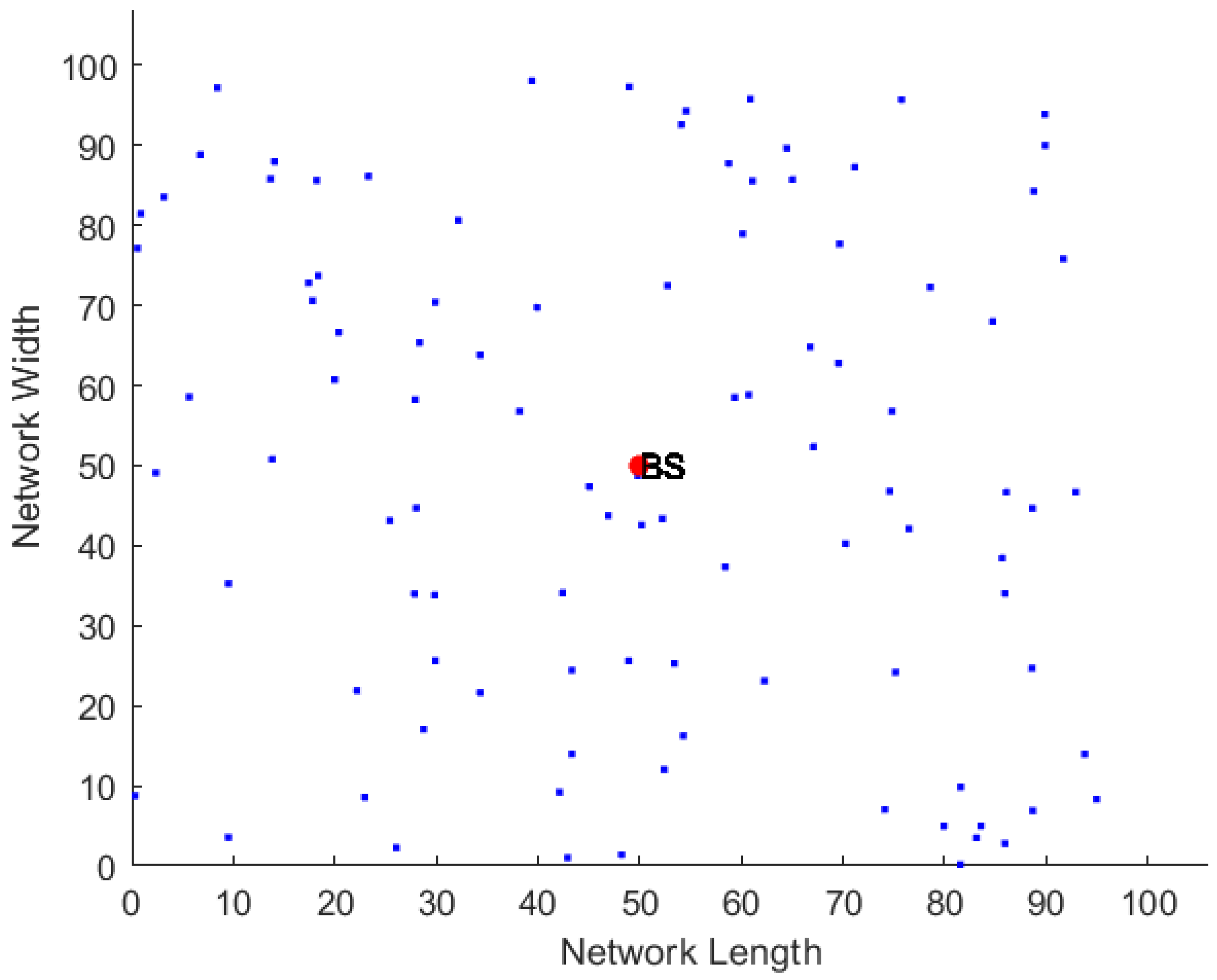
In this section, we discuss the different models that represent the proposed proactive approach. We consider a WRSN of area A in which there is a set S of N sensor nodes, $S=\{s_1,s_2,s_3,..,s_N\}$, that are deployed randomly and these nodes are responsible for sensing and monitoring A. All sensor nodes start their tasks with initial maximum energy $E_{in}$.

3.1. Network Model

We assume a WRSN which is composed of a BS, a set of N homogeneous rechargeable sensor nodes randomly deployed in the sensing field, and a single MC that is used to recharge the sensor nodes using a multi-node charging mode. The sensing area A shown in Figure 2 is divided into hexagonal cells as shown in Figure 3, where each cell can contain any number of sensor nodes. The figure depicts the network area, which is partitioned into hexagonal cells to ensure that any sensor node within its cell can receive charging power from the MC when it stops at the center of that cell. This approach was verified in [36] where it was demonstrated that, by visiting the center of the cell, the MC can charge all the sensor nodes within it, given that the length of the hexagonal cell side is equivalent to the charging range of the MC. It is worth emphasizing that the segmentation of the area into hexagonal cells is performed virtually by the BS and it does not depend on the BS location or any other factors such as the distribution density of nodes. Segmentation is used to determine the center point (location) of each cell to which the MC should move to recharge the nodes of that cell. For example, hexagonal cells can be centered in the BS and spread over the concerned region, and this will not have an effect on the functionality of the proposed approach.

It is assumed that the BS has sufficient energy and communication capabilities to transmit any data directly to the MC. The MC, as a mobile robot, is equipped with communication and processing components, in addition to a wireless power transmission mechanism that allows it to be powered by a rechargeable battery at the service station (SS). It is assumed that every sensor node has a stationary position that is known by the BS. Moreover, a wireless power receiver is built within each sensor node to receive the electricity delivered by the MC for recharging. Furthermore, it is assumed that the MC and the sensor nodes use GPS to determine their locations.

After the sensor nodes start communication with each other, every sensor node i can calculate at any time how much power it uses ($PCRi$) and it transmits this value to the BS when it sends the sensed data to the BS every determined period $T_d$ which is assumed to be 1 s in this study. The BS provides the MC with the coordinates of each cell’s center, as it already possesses all the necessary information about the geo-locations of the cells and their members, as will be explained in the upcoming sections.

3.2. Energy Consumption Model

The proposed method makes use of the multi-hop routing model defined in [37]. The multi-hop routing in wireless sensor networks refers to the process of transmitting data between sensor nodes through intermediate nodes rather than directly to a central base station. This approach allows for more efficient communication over longer distances, as data can be relayed through multiple nodes, thereby extending the network’s range and improving connectivity. In this model, which is also explained in more detail in [38], the power consumption rate for transmission by a given node when it forwards a flow rate $F_{ij}$ from node i to node j, is given as follows:

$$T{R}_i=C_{ij}\times F_{ij}$$

(1)

where $C_{ij}$ is the one unit of data transmission cost from node i to node j in terms of energy usage, and it is modeled as follows:

$$C_{ij}=\beta 1+(\beta 2\times D_{ij}^{\alpha })$$

(2)

where $\beta 1$ is a constant term independent of distance, $\beta 2$ is a coefficient of the term that depends on distance, $\alpha$ is the path-loss index, and $D_{ij}$ is the distance between i and j. The value of $F_{ij}$ used here is a random value between 1 and 10 kbps.

If the sending node i is the nearest among its neighbors to the BS, the power consumption rate at node i for transmitting its own flow rate $F_{iB}$ to the BS is calculated as follows:

$$T{R}_i=C_{iB}\times F_{iB}$$

(3)

where $C_{iB}$ is how much energy is used to send one unit of data from node i to the BS.

The power consumption rate for reception at node i ($R{R}_i$) is calculated as follows:

$$R{R}_i=\rho \times \sum _{k\in N}^{k\ne i}\left(F_{ki}\right)$$

(4)

where $\rho$ is the power consumption coefficient for receiving data [38]. Then, the overall power consumption rate during transmission and reception $PC{R}_i$ at node i is given as follows:

$$PC{R}_i=R{R}_i+T{R}_i$$

(5)

3.3. Charging Model

In this paper, the charging model proposed in [39] is also used as follows:

$$P_r={\displaystyle \frac{G_s{G}_r\eta }{L_p}}{\left({\displaystyle \frac{\gamma }{4\pi (d+\beta )}}\right)}^2{P}_0$$

(6)

where $P_r$ is the received power, $P_0$ is the source power, $G_s$ and $G_r$ are the source and receiver antenna gain, respectively, $\eta$ is the rectifier efficiency, $L_p$ is polarization loss, $\gamma$ is the wavelength, d is the distance between the charger and the receiver, and $\beta$ is a variable that modifies the Friis’ free space equation for transmission over short distances, in a standard commercial RFID reader. $G_s$, $G_r$, $\eta$, $\gamma$, and $L_p$ have the values 8 dBi, 2 dBi, $0.125$, $0.33$ m, and 3 dB, respectively.

All parameters in Equation (6) are constant values based on the device settings and the environment, except the d value. Experimental evidence has demonstrated that this model, which is based on Friis’ free space equation, is a good description of charged energy [39]. This charging model was simplified in [40] for easy description as in the following equation:

$$Ch{R}_i={\displaystyle \frac{\lambda }{{(D_{m{c}_i}+\beta )}^2}}$$

(7)

The charging rate for sensor node i, denoted as $Ch{R}_i$, represents the amount of energy that the sensor node can be charged per second when the MC is stationary at a distance $D_{m{c}_i}$ from the sensor node. The value of $\lambda$ represents the constant environmental parameters including $P_0$, $G_s$, $G_r$, $L_p$, $\eta$, and $\gamma$. The value of $\beta$ is the same as in Equation (6).

Using the $Ch{R}_i$ value, the time required to fully charge a single node i depends on its residual energy value ${E_{res}}_i$ and the maximum energy capacity $E_{in}$ as follows:

$${T_F}_i={\displaystyle \frac{(E_{in}-{E_{res}}_i)}{Ch{R}_i}}$$

(8)

Furthermore, the duration for which node i remains operational (${T_S}_i$) is subject to a certain threshold value ($E_{th}$). The ${T_S}_i$ value is calculated using the following equation:

$${T_S}_i={\displaystyle \frac{({E_{res}}_i-E_{th})}{PC{R}_i}}$$

(9)

The value of $E_{th}$ is predetermined and it represents the energy value at which the sensor node is considered to be in a critical situation and close to energy depletion. It is the same value that is used in on-demand systems such that when the sensor node reaches this threshold, it sends a charging request to be recharged.

4. The Proposed Proactive Charging Strategy

The proposed proactive charging strategy is motivated by various goals, including minimizing the node energy depletion, decreasing the node failure rate, reducing the overhead control messages within the network by eliminating the need for energy requests, and preventing charging latency.

After deploying the sensor nodes randomly in the sensing area, the required routing and topology information are constructed using the multi-hop routing protocol [37], wherein each sensor node is considered as a relay node which uses its neighboring nodes to relay the data to the BS. Then, the nodes start their task by sensing the surroundings and transmitting the sensed data to the BS. At the beginning of network operation, the MC is assumed to be located at the service center, while the BS is at the center of the network region.

The amount of data that passes via each sensor node i determines how much power it will consume ($PC{R}_i$), which is used by the sensor node to compute its residual energy (${E_{res}}_i$). The sensor node then uses the ${E_{res}}_i$ value to calculate the time-space that allows it to stay alive (${T_S}_i$) before its remaining energy reaches a predetermined threshold value ($E_{th}$). The ${E_{res}}_i$ and ${T_S}_i$ values are sent to the BS by appending them to the sensed data; therefore, the sensor nodes avoid using extra overhead control messages to send the ${E_{res}}_i$ and ${T_S}_i$ values.

After receiving the $E_{res}$ values from all sensor nodes, the BS utilizes them to calculate the time (${T_F}_i$) that is necessary for each sensor node i to achieve complete charging depending on its distance from the cell’s center, which in turn controls the rate of charge it will receive from the charger ($Ch{R}_i$). These calculations enable the BS to determine which cell the MC is going to visit next in order to recharge its sensor nodes. The decision will not be based on a single node but rather on all the calculated values for all nodes in the entire cell.

Proactive Charging Process

The proposed proactive charging method operates on the premise that the BS identifies sensor nodes that require charging before they reach a critical state, thus eliminating the need for the nodes to request charging from the MC. The following steps make up the proactive process:

• Each node i defines its power consumption rate $PC{R}_i$ once network communication has begun according to Equation (5). Then, it uses its $PC{R}_i$ value to compute its residual energy value ${E_{res}}_i$ according to the following equation:

  $${E_{res}}_i=E_P-(PC{R}_i\times T_p)$$

  (10)

  where $E_p$ is the previous value of the residual energy and $T_p$ is the time passed since the last calculation of ${E_{res}}_i$. The sensor node will use the residual energy value to calculate the period of time that permits it to remain safe (${T_S}_i$) above the energy threshold value according to Equation (9). After that it sends its ${E_{res}}_i$ and ${T_S}_i$ values to the BS.
• The BS uses the ${E_{res}}_i$ and ${T_s}_i$ values it has received from all nodes to determine the following values:
  • ${T_F}_i$: The amount of time required to fully charge each node i using Equation (8).
  • ${C_{T_D}}_j$: The time that each cell j needs to be charged. The ${C_{T_D}}_j$ value is calculated by averaging all the ${T_F}_i$ values for its $m_j$ members as follows:

    $${C_{T_D}}_j={\displaystyle \frac{{\displaystyle \sum _{i=1}^m}{T_F}_i}{m_j}}$$

    (11)
  • ${C_{T_S}}_j$: The time that allows each cell j to stay above the threshold value (time-space to stay safe) by taking the average of all ${T_S}_i$ values for its $m_j$ members as follows:

    $${C_{T_S}}_j={\displaystyle \frac{{\displaystyle \sum _{i=1}^{m_j}}{T_S}_i}{m_j}}$$

    (12)
  Then, the BS begins selecting the next cell ($C_N$) to visit and recharge its nodes. This cell is the one that has the shortest amount of time to be safe before encountering a critical condition in which one of its members might enter the dead state, as follows:

  $$C_N=\underset{\forall s\in S_j}{min}{C_{T_S}}_j$$

  (13)
  After making the decision to select the next cell, the BS sends the following information about $C_N$ to the MC:
  • The coordinates of its center ($X{c}_N$, $Y{c}_N$).
  • Its charging duration need ${C_{T_D}}_N$.
  The BS then determines the scheduling time for recharging the next cell $T_{sch}$, which is determined by the period needed for the MC to travel to and recharge the target cell as in the following equation:

  $$T_{sch}=T_r+{C_{T_D}}_N$$

  (14)

  where ${C_{T_D}}_N$ is the charging duration for the chosen cell and $T_r$ is the time the MC needs to arrive at this cell, where $T_r$ is calculated as follows:

  $$T_r={\displaystyle \frac{D_N}{Vel}}$$

  (15)

  where $D_N$ is the distance between the MC’s present position and the center of the next cell, and $Vel$ is the MC’s velocity.
• After acquiring the required information from the BS, the MC will use the cell center coordinates to know its next destination cell and use the charging duration value to know how long it will stay charging that cell.

By doing this, the BS prevents nodes from reaching critical energy levels before they become a problem, and it avoids the need to relay messages or requests from nodes whose energy has reached or is on the verge of reaching critical energy levels.

Algorithms 1, 2 and  3 show the pseudo-codes for the operation of a sensor node i, the BS, and the MC, respectively.

Algorithm 1 Sensor node i Working Process

Input: $T_d$      Output: $MESSAGE$ 1: $T\leftarrow$ Start node i timer 2: $k=1$ 3: $F_{iB}\leftarrow$ sense the environment 4: $C_{iB}\leftarrow$ Energy to send one unit of data from node i to BS 5: while True do 6:     if $(T=k.T_d)$ then 7:         $k=k+1$ 8:         $MESSAGE\leftarrow$ Prepare Data to send(FiB) 9:         $\mathit{TNR}=\mathit{0}$ 10:         for   each neighbor node l of i do 11:             if There is a message from l then 12:                $MESSAGE\leftarrow \mathit{Append}($Fli) 13:                $TNR=TNR+F_{li}$ 14:            end if 15:         end for 16:         $T_{Ri}=C_{iB}\times F_{iB}$ 17:         $R{R}_i=\rho \times TNR$ 18:         $PC{R}_i=R{R}_i+T_{Ri}$ 19:         $T_{Si}$ = ${\displaystyle \frac{(E_{resi}-E_{th})}{PC{R}_i}}$ 20:         $E_{resi}=E_p-(PC{R}_i\times T_p)$ 21:         $MESSAGE\leftarrow \mathit{Append}($Eresi,TSi) 22:         send MESSAGE to the next relay node 23:     end if 24: end while

Algorithm 2 BS Working Process

1: Divide the network into hexagonal cells 2: $M\leftarrow$ Number of Cells 3: for k = 1 to M do 4:     $m_k\leftarrow$ Number of sensor nodes in Cell k 5:     $(X_k,Y_k)\leftarrow$ Center location of Cell k 6: end for 7: while True do 8:     Wait Until Receiving data from all nodes 9:     for i = 1 to N do 10:         $T_F\left(i\right)\leftarrow \mathit{find}$ TF $for node$ i $using$ Equation (8) 11:     end for 12:     for k = 1 to M do 13:         $TS=0$ 14:         $TD=0$ 15:         for j = 1 to N do 16:            if j is a member in Cell k then 17:                $TS=TS+T_S\left(j\right)$ 18:                $TD=TD+T_F\left(j\right)$ 19:            end if 20:            $C_{T_S\left(k\right)}$ = ${\displaystyle \frac{TS}{m_k}}$ 21:            $C_{T_D\left(k\right)}$ = ${\displaystyle \frac{TD}{m_k}}$ 22:         end for 23:     end for 24:     find the next time to choose a cell $T_{sch}$ by Equation (14) 25:     Send ($X{c}_N$, $Y{c}_N$) and ${C_{T_D}}_N$ to the MC 26: end while

Algorithm 3 MC Working Process

1: $(X,Y)\leftarrow \mathit{Next} \mathit{location} \mathit{of} \mathit{the} \mathit{MC}$ 2: Wait for a message from the BS 3: $Message\leftarrow$ MC Receives a message from the BS 4: if $Message$ contains $C_N$ $information$ then 5:     $(X,Y)\leftarrow (X{c}_N,Y{c}_N)$ 6:     move to (X,Y) 7:     start charging nodes in $C_N$ for a period of ${C_{T_D}}_N$ s 8: end if 9: Goto step 1

5. Experiment and Performance Evaluation

In this section, the effectiveness of the proposed approach is evaluated, and the results are thoroughly studied and presented. The recharging process is performed every $T_d$ seconds. Firstly, we discuss the metrics that are used to evaluate the proposed approach. Then, we discuss the charging techniques that we compare our approach with. After that, we discuss the experiment setup and present the simulation results.

5.1. Performance Metrics

To evaluate how successfully charging plans perform in a WRSN, different metrics can be employed. A charging strategy often seeks to maximize and/or minimize one or more metrics while also satisfying some restrictions that serve as limitations. It is important to remember that some metrics are inherently contradictory. For instance, if the sensor nodes desire to experience a small charging delay, the MC’s service cost might increase. Moreover, using fewer MCs could shorten the network lifetime [41]. The following metrics are used to evaluate the performance of the proposed proactive recharging strategy:

• Network Lifetime: Because the sensor nodes have tiny batteries, the network lifetime is a crucial performance metric. The work in [42] proposed several definitions for the network lifetime. It could be defined, for instance, as how long it will take before the first sensor node, the last sensor node, or a predetermined percentage of sensor nodes die. In this paper, the network lifetime is expressed by the following sub-metrics:
  • The period until the death of the first node.
  • The overall number of alive nodes after a certain number of rounds.
  • The total remaining energy in all sensor nodes after a certain number of rounds.
• Service Cost (SC): The authors of [43] evaluated the efficiency of the charging technique using the service cost metric which is defined as the sum of the MC’s charging-related travel distances. The SC typically increases with an increase in the number of MCs, sensor nodes, and network size. Since the energy used for travel is regarded as overhead, it is preferred to use a low-service cost strategy. Assume the MC will charge $Nr$ sensor nodes, the $SC$ is represented by the path length the MC will use to recharge these sensor nodes and it is calculated as follows:

  $$SC={\displaystyle \sum _{i=1}^{Nr}}T{T}_i\times Vel$$

  (16)

  where $T{T}_i$ is the traveling time of the MC to move from its current location to the location of sensor node i, and $Vel$ is the MC velocity.
• Energy Usage Efficiency (EUE): It is generally recognized that the most efficient method for recharging depleted sensor nodes is one with a high energy usage efficiency rating. Therefore, and since the MC carries limited energy in each cycle, EUE is considered an important metric to measure how any proposed recharging strategy is efficient [44]. EUE is defined as the ratio of the energy used for charging the sensor nodes to the total energy of the MC. EUE is calculated as follows:

  $$EUE={\displaystyle \frac{Ep}{Ep+Eo}}$$

  (17)

  where $Ep$ is the payload energy which represents the overall amount of energy that the MC transmitted to the sensor nodes for charging them during the charging process. $Eo$ is the overhead energy which represents the consumed energy during the MC traveling to all recharged sensor nodes.
• Failure Rate (FR):The failure rate reflects a charging technique’s ability to recover energy to keep sensor nodes from running out of energy [45]. For prolonging the network lifetime, it is preferable to use a recharging strategy with little failure. The FR metric is calculated as follows:

  $$FR={\displaystyle \frac{N_d}{N}}$$

  (18)

  where $N_d$ is the number of dead sensor nodes and N is the total number of sensor nodes.
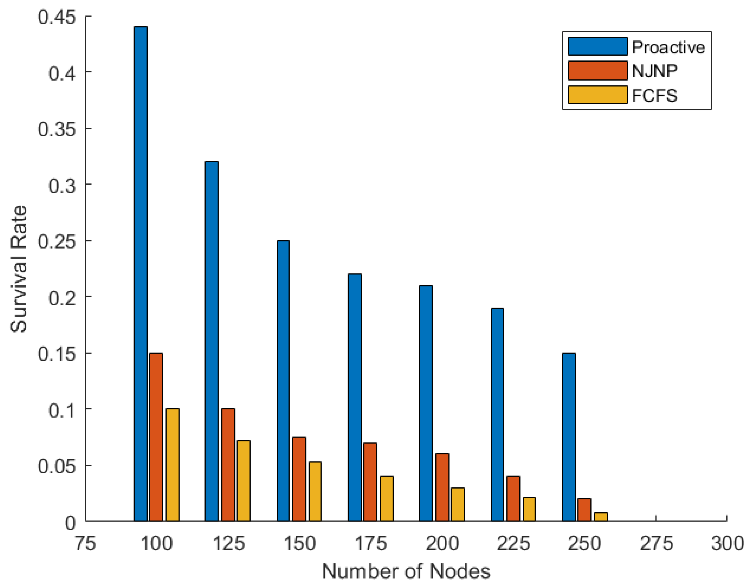
• Survival Rate (SR): This is a metric used to evaluate the effectiveness of the charging system [46]. The SR refers to the proportion of active sensor nodes to all nodes. It is recommended to use a charging system that has a high rate of survival to guarantee an extended operational duration for the network. The SR is usually measured after running the network over a duration of time and is calculated as follows:

  $$SR={\displaystyle \frac{N_s}{N}}$$

  (19)

  where $N_s$ is the number of surviving nodes and N is the total number of sensor nodes. The FR and SR values are opposite and complement each other; therefore, $FR$+ $SR$ = 1.

5.2. Charging Techniques Used in the Comparison

The performance of the proactive approach was compared against two main common on-demand techniques: First Come First Serve (FCFS) [47] and Nearest Job Next with Preemption (NJNP) [48]. In FCFS, charging requests from nodes are satisfied in the order in which they arrive, whereas, in NJNP, the MC selects the subsequent charging node which is the spatially nearest demanding sensor node, as explained in the following sub-sections.

5.2.1. First Come First Serve (FCFS) Technique

The FCFS algorithm is a straightforward scheduling method used in wireless rechargeable sensor networks. In this approach, sensor nodes send charging requests when their energy levels drop below a predefined threshold, typically around 20%. These requests are stored in a queue and processed in the order they are received. The MC travels to the location of each sensor node to perform the charging, which occurs for a fixed duration. While FCFS is easy to implement and ensures that all requests are eventually addressed, it may lead to inefficiencies, as urgent requests can be delayed if they arrive after less critical ones. In the FCFS technique, the charging requests are handled depending on their arrival time. In particular, the FCFS technique only uses temporal parameters to establish the charge schedule for incoming charging requests. Unfortunately, because the charging schedule of the MC is established by neglecting the geographic locations of the nodes that ask for recharging, the MC might have to move across the spatial domain unnecessarily. Therefore, this could worsen the charging delay and shorten the network’s lifetime.

It is worth noting that a modification has been applied to the operation of the FCFS in our paper in order to provide fairness when it is compared to our proposed proactive approach. The original version of the FCFS algorithm was proposed based on the one-to-one charging model in which the MC charges each node alone. However, the model that is used in our proposed method is a one-to-multiple charging model. Therefore, the FCFS algorithm has been used in this paper using the one-to-multiple model. This means that whenever a node in a given cell requests energy from the MC and the node’s time of the request is ready to be fulfilled, the MC moves to that node’s cell and starts charging all the sensor nodes in that cell.

5.2.2. Nearest Job Next with Preemption (NJNP) Technique

To resolve the issues with FCFS, the authors of [48] proposed the NJNP algorithm which enhances the charging process by incorporating priority levels for sensor nodes based on their remaining energy and the criticality of their tasks. Similar to FCFS, sensor nodes send requests when they reach a reasonable energy threshold. However, NJNP prioritizes the nearest high-priority sensor when the charging vehicle is ready to service a request, minimizing the travel distance and reducing service interruptions. This algorithm requires more complex implementation due to the need for dynamic priority management but offers improved efficiency by addressing urgent needs promptly.

In the NJNP technique, the next-to-be-charged node can be switched out for the closest requesting node by the MC. In other words, the MC chooses a new node to charge based on the geographical positions of the requesting nodes once a sensor node i has been fully charged or after it has received a new charging request. Incorporating the concept of preemption during the charging process has effectively resolved the drawbacks associated with the FCFS technique.

However, preemption can introduce new challenges in this process, such as the difficulty of the sensor’s starvation as a result of numerous preemption procedures. Moreover, there is the issue of technique inconsistency for large-scale WRSNs. It should be noted that the same modification that was considered on the FCFS algorithm was also considered on the NJNP algorithm in the proposed experiment in terms of applying the technique to the one-to-multiple charging model instead of the one-to-one model.

5.3. Design of the Experiment

To assess the effectiveness of the proposed proactive charging strategy, a set of experiments was conducted on a PC running Microsoft Windows 10 with 8 GB Memory and an Intel Core i3 processor using the MATLAB R2019 simulation tool for implementing the codes of the proposed proactive, the FCFS, and the NJNP approaches. For evaluation of the proactive scheme, 100 to 250 sensor nodes are dispersed at random in a sensing field of area A = $100\times 100$ m² with an increase of 25 nodes per step. One MC is assumed to refuel the energy for the nodes and has a service station at location (0,0) in A. The BS is located at the center of the sensing field.

The parameter values for the power consumption model, $\rho$, $\beta 1$, $\beta 2$, and $\alpha$, in addition to the hexagonal side length of the MC’s charging range $R_{MC}$ that were used in [36] are also used in this study. The values of the charging model’s parameters $\lambda$ and $\beta$ that were used in [40] are also used in this paper. Furthermore, the parameter values related to the MC such as its velocity $Vel$, the overload energy $E_o$, and the payload energy $E_p$ are used the same as in [40]. The communication range of the sensor nodes, $R_c$, was chosen to be 50 m. The parameters and their values used in the simulation are listed in

Table 2. The parameters used with their values.

Parameter	Description	Value
N	Total number of nodes	100–250
A	Area size	$100\times 100$ m2
$\rho$	The power consumption coefficient for receiving data	50 nJ/b
$\beta 1$	Constant in Equation (2)	50 nJ/b
$\beta 2$	Constant in Equation (2)	0.0013 pJ/b/m4
$\alpha$	Path-loss index	4
$\lambda$	Constant in Equation (6)	36 J.m2/s
$\beta$	Constant in Equation (6)	30 m
$F{R}_i$	Data flow rate for sensor i	[1,10] kb/s
$E_{in}$	Initial energy for each sensor	2 J
$R_{MC}$	Charging range of the MC	3 m
$R_c$	Sensor’s communication range	50 m
$E_{th}$	Energy threshold value	0.6 J
$Vel$	Velocity of MC	5 m/s
$E_O$	MC’s overhead energy	0.1 J/m
$E_p$	MC’s payload energy	10 J/s
$E_{MC}$	MC’s initial energy	400 J
$TST$	Total simulation time	5000 s

. For configuring the experiments with the energy threshold value $E_{th}$, which is used in calculating the ${T_S}_i$ value as given in Equation (9), $E_{th}$ was set to 30% of the maximum energy of the sensor node as this ratio was used in [15].

5.4. Experiment Results

The results of the simulation experiment are reported in this section. As previously stated, the primary goal of implementing a recharging technique in a given WRSN is to prolong the network operation. However, the performance of the recharging approach is influenced by the path that the MC takes while recharging the sensor nodes. As a result, multiple metrics are presented to assess the impact of the MC path on the recharging approach.

When the BS determines which cell will be recharged next, the MC begins moving to visit that cell and then stops at its center location and starts charging the nodes inside that cell. The path length of the MC is calculated starting when it moves from the service station to the center of the first chosen cell, then to the center of the next cell, and so on.

5.4.1. Network Lifetime

In comparison to the FCFS and NJNP strategies, the following measures are utilized to represent how well the proposed proactive strategy performs in terms of network lifetime:

• The period until the death of the first node.
  The duration from the beginning of the network operation until the death of the first node is used as a measure of the network lifetime. Figure 4 shows the network lifetime when the proposed proactive approach is used in comparison to the FCFS and NJNP approaches and when the network operates without using any charging method.
  Table 3. The percentage of improvement of the proactive, FCFS, and NJNP approaches over the no-charging approach.

  Number of Nodes	Proactive	NJNP	FCFS
  100	752%	118%	109%
  125	610%	103%	81%
  150	540%	93%	80%
  175	497%	69%	62%
  200	472%	59%	48%
  225	388%	22%	19%
  250	297%	6%	6%

  shows the percentage of improvement of the proactive, FCFS, and NJNP approaches in reference to the no-charging method during the period until the death of the first node. The improvement is calculated as follows:

  $$Improvement={\displaystyle \frac{T_N-T_R}{T_R}}\times 100\%$$

  (20)

  where $T_N$ is the time of the first dead node in the proactive, NJNP, or FCFS approach and $T_R$ is the time of the first dead node in the reference technique (no charging). The findings presented in the table demonstrate that the major contribution of the proactive approach in extending the network lifetime measured by the time until the death of the first sensor node outperforms the FCFS and NJNP approaches significantly. For example, the proactive approach reports a 752% improvement when the number of deployed sensor nodes is 100, whereas the FCFS and NJNP approaches report 118% and 109%, respectively.
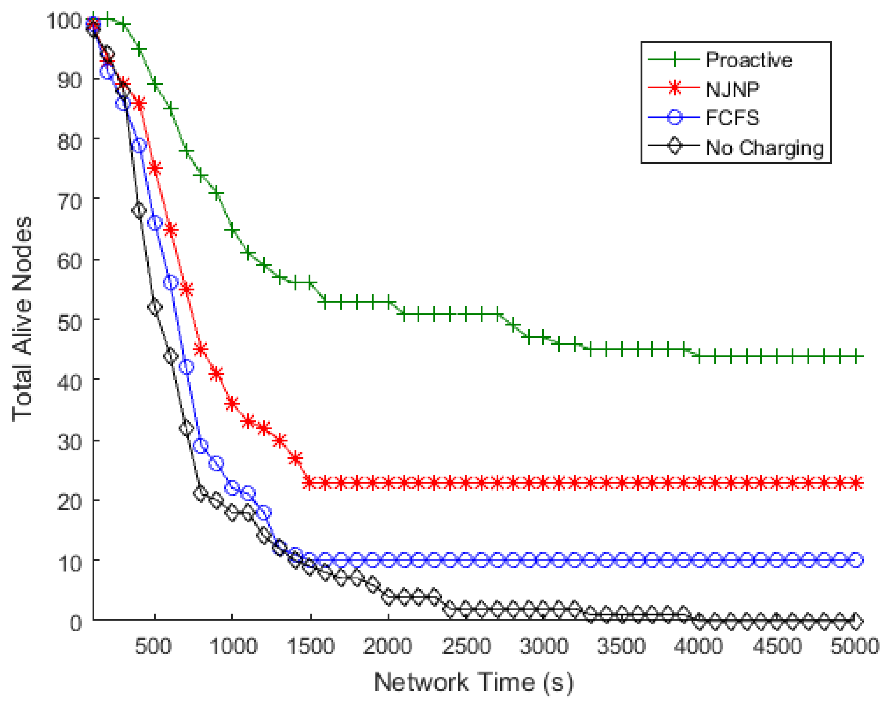
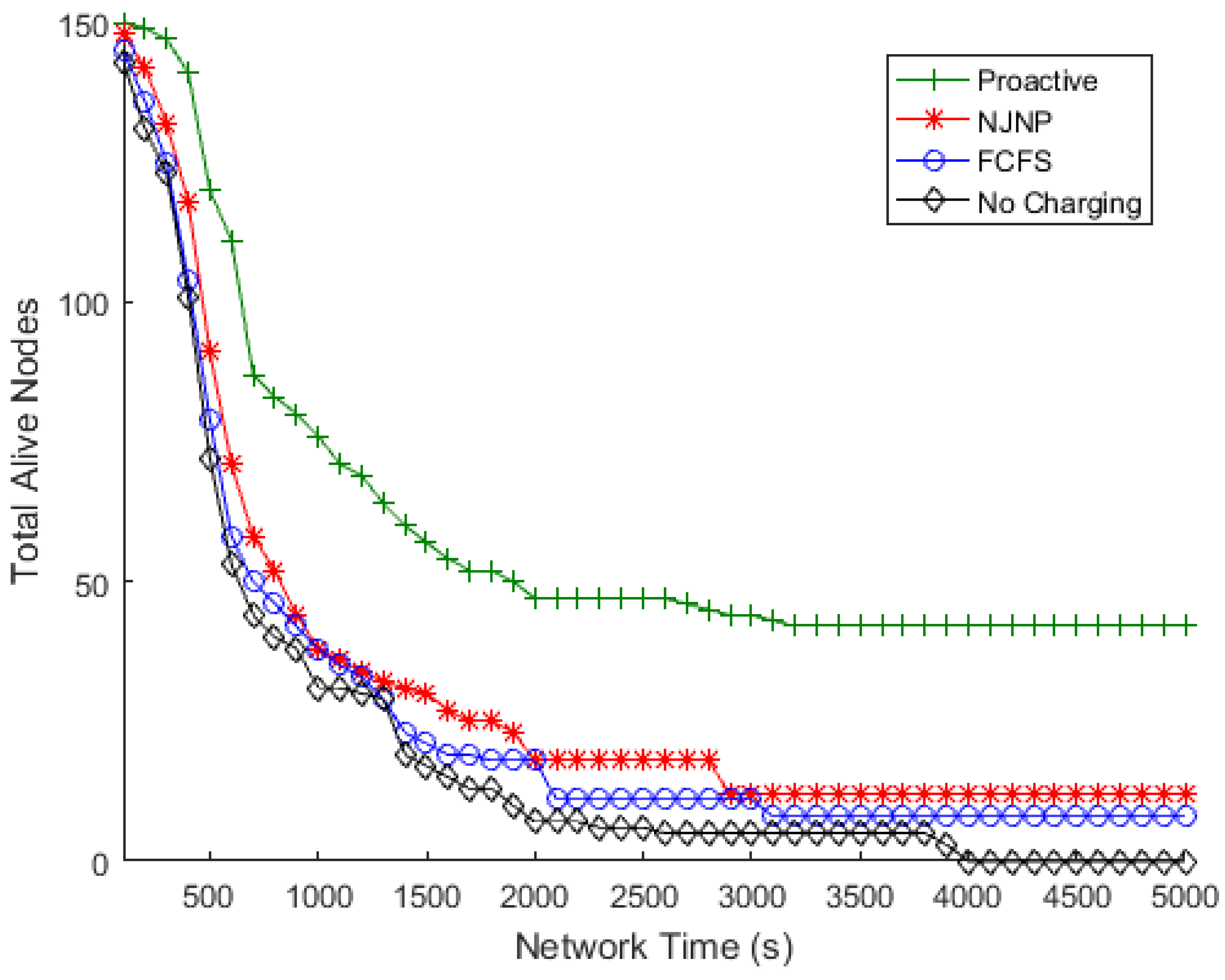
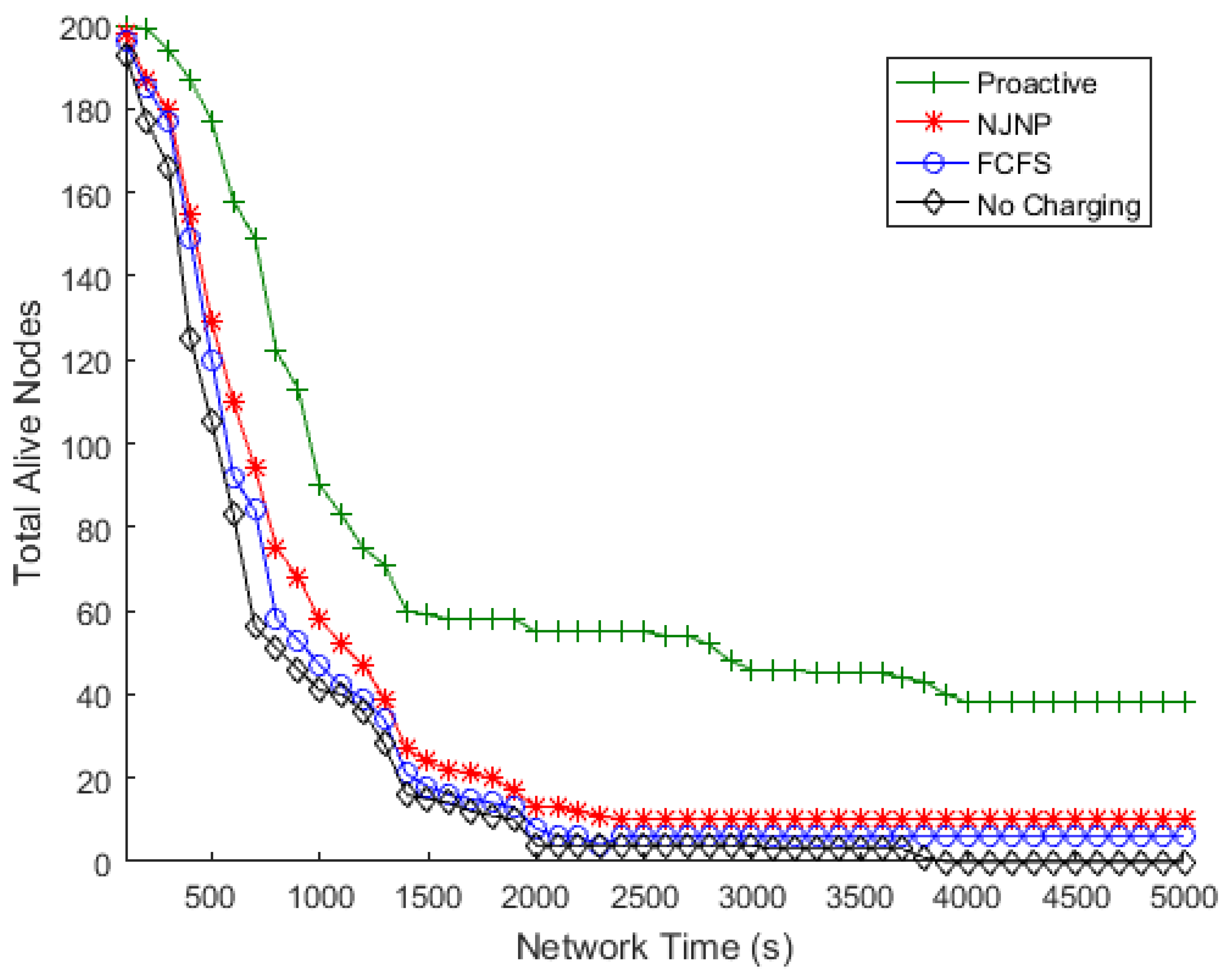
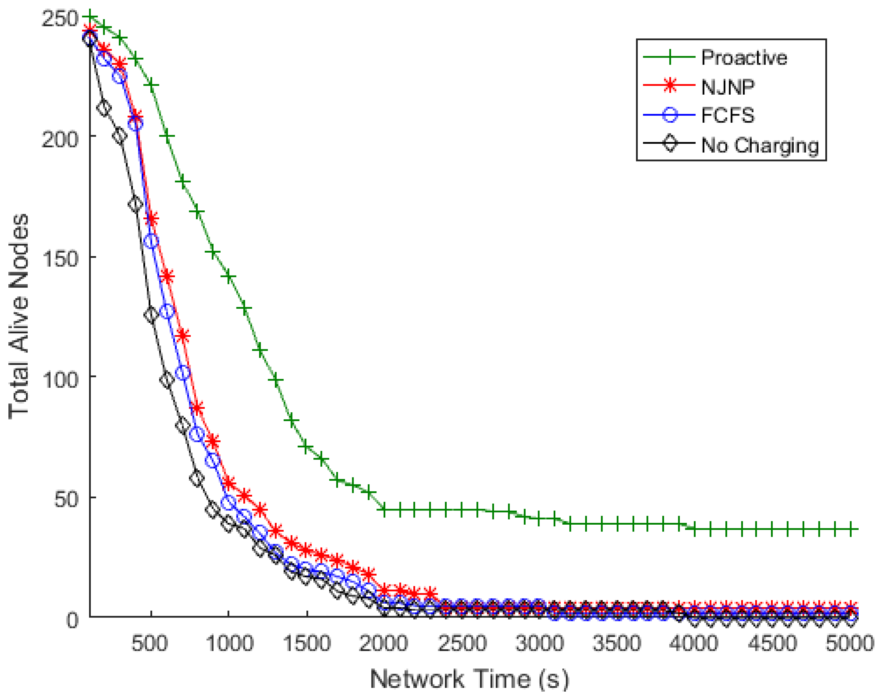
• Total number of alive nodes.
  The number of nodes that remain alive at the end of the simulation demonstrates the network’s capacity to live longer. Figure 5, Figure 6, Figure 7 and Figure 8 show the numbers of alive nodes over time when the number of deployed sensor nodes (N) is 100, 150, 200, and 250, respectively.
  Figure 9 depicts the overall number of nodes that were still alive after the end of the simulation versus the number of deployed sensor nodes using the proactive approach compared to the FCFS and NJNP methods. It is worth noting that, when no charging was used, all nodes were dead by the end of the simulation. Figure 9 also shows that, despite the number of deployed nodes, the proactive approach succeeds in maintaining a high level of surviving nodes compared to the NJNP and FCFS charging techniques.
  Figure 9 shows that the total number of alive nodes decreases as the number of nodes increases. This trend can be attributed to several factors inherent to WSNs with densely deployed sensor nodes. First, as the number of nodes grows, the total energy demand of the network increases significantly due to higher data transmission and sensing activities. While the proactive charging strategy anticipates and addresses energy needs, the limited capacity of the MC makes it challenging to meet the energy demands of all nodes in densely populated WSNs, leading to some nodes depleting their energy before being recharged. Second, the higher node density results in increased competition for the MC’s charging resources, causing delays for nodes that are farther from the MC or in less frequently visited cells. Additionally, the service cost (SC), which represents the MC’s travel distance, increases with the number of nodes, reducing the MC’s energy usage efficiency (EUE) and leaving less energy available for charging. Finally, the threshold-based approach used by the proactive charging strategy may struggle to handle the simultaneous energy demands of many nodes in densely populated WSNs, leading to a higher number of nodes dying before they are recharged. Despite this trend, the proactive charging strategy consistently outperforms the baseline methods (FCFS and NJNP) in terms of the number of alive nodes, demonstrating its effectiveness even in densely populated WSNs.
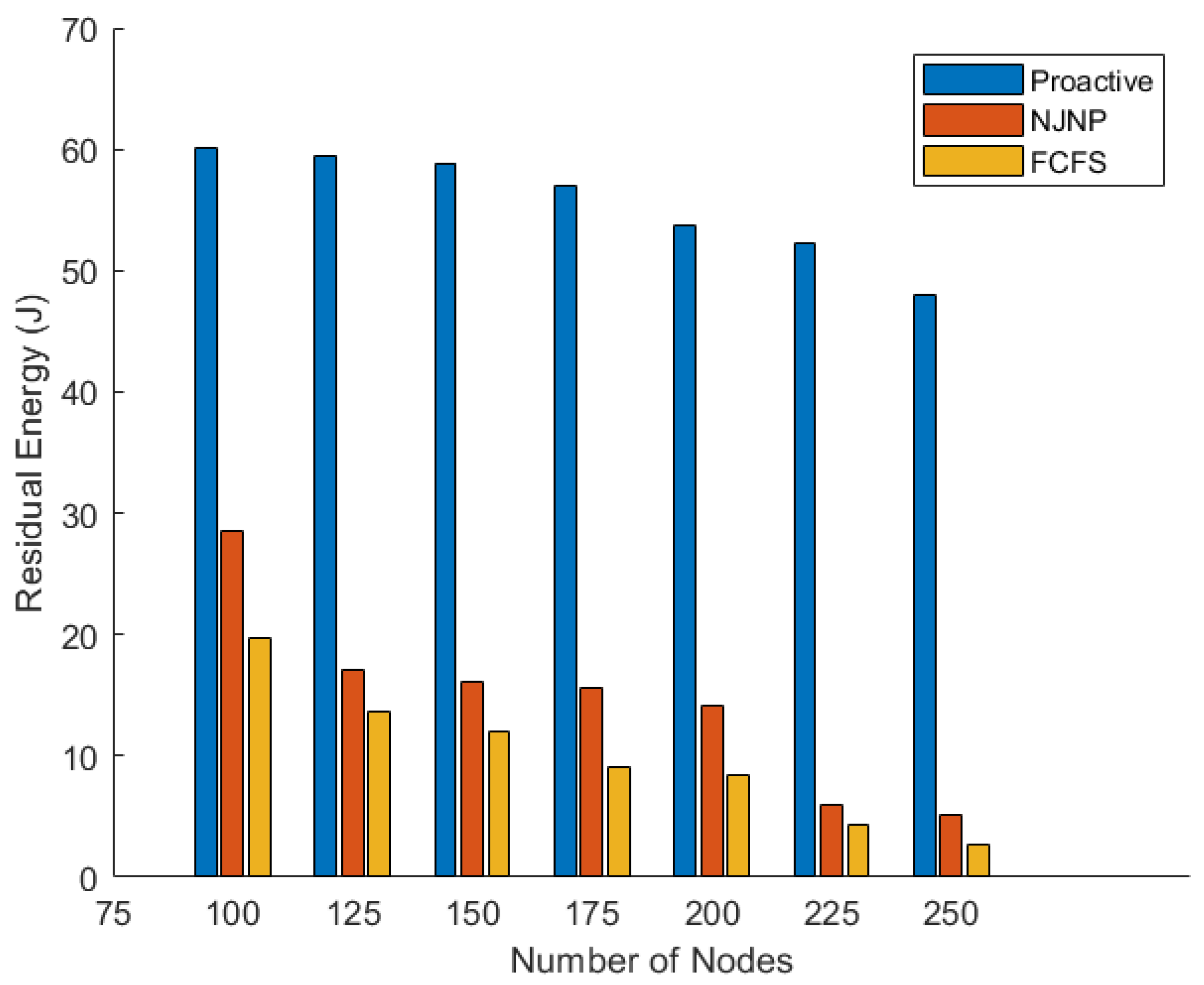
• Total amount of residual energy.
  The level of residual energy in sensor nodes reflects another point of view for the time that the network can remain operational. Figure 10 depicts the total residual energy in the sensor nodes at the end of the simulation. In comparison to the NJNP and FCFS techniques, the findings shown in the figure show that the proposed approach was able to keep the most energy in the nodes that remained alive and thus capable of continuing to operate.

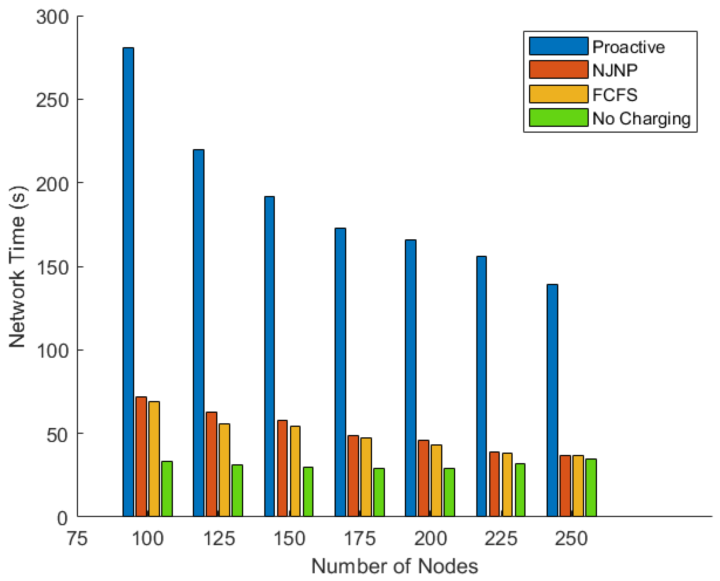
5.4.2. Service Cost (SC)

The service cost represents the total distance that the MC travels during the network operation in order to recharge the sensor nodes. The SC was evaluated for the first 1000 s of the simulation time. Figure 11 shows the SC of the MC in the proactive charging approach compared to the FCFS and NJNP approaches when the number of nodes was 100, 125, 150, 175, 200, 225, and 250. The figure shows that the SC of the MC in the proactive approach is high compared with the NJNP and FCFS approaches. This can be justified because the MC in the proactive approach begins moving from one cell to another to recharge the nodes in advance. However, in the NJNP and FCFS approaches, the MC does not move unless a request is received from a node.

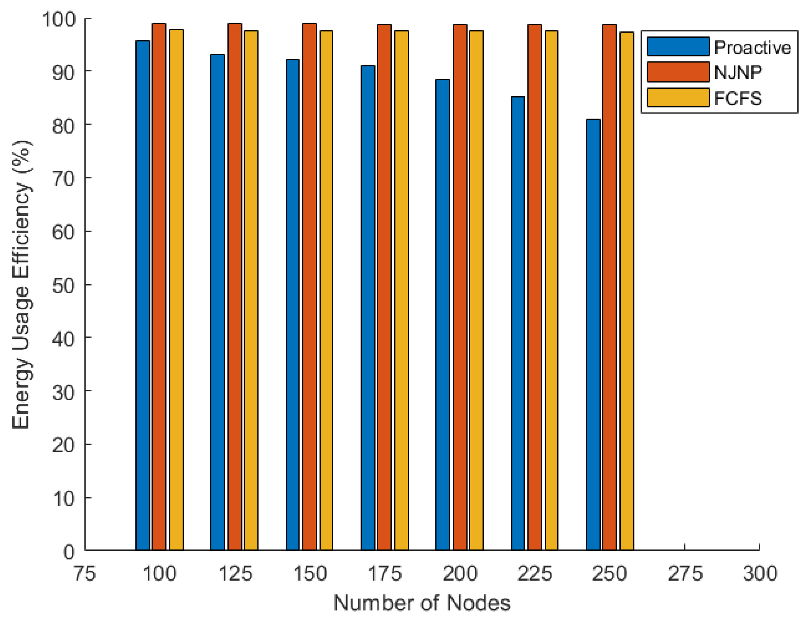
5.4.3. Energy Usage Efficiency (EUE)

Figure 12 shows the EUE metric of the proposed approach compared with the FCFS and NJNP approaches at different numbers of the deployed sensor nodes. This metric is recorded at the end of the simulation (after 5000 s). The figure shows that the MC efficiency in terms of EUE in the proactive approach is lower compared with the FCFS and NJNP approaches. This can be justified because the MC in the proactive approach begins moving and charging early despite the fact that the nodes did not lose a large amount of energy. Therefore, it spends some of its energy moving from one cell to another, putting a moderate amount of energy in all cells to keep a large number of cells alive. However, in the NJNP and FCFS systems, the MC will move to a given cell only when a node inside that cell requires a large amount of energy, which means the MC will use more energy in charging compared to the amount of energy used in traveling. The figure also indicates that the MC efficiency is highest in the NJNP approach. This is because, in the NJNP approach, the MC moves towards the nearest cell and thus it travels a shorter distance compared with that traveled by the MC in the FCFS approach.

5.4.4. Failure and Survival Rates

Figure 13 shows the FR versus the number of deployed sensor nodes where this metric is calculated at the end of the simulation (after 5000 s). As shown in the figure, the minimum FR is in the proactive approach which indicates its ability for keeping a large number of nodes active compared with the FCFS and NJNP approaches. NJNP is the second approach that has a lower FR followed by the FCFS approach. This conclusion is also emphasized in Figure 14 which shows the SR versus the number of sensor nodes.

6. Discussion

The results reveal that the proposed approach significantly increases the network’s lifespan. After computing the enhancement rate for each case of the number of deployed sensor nodes, beginning with 100 sensors and increasing to 250 sensors, the proposed proactive scheme increased the time before the first sensor failure by around 500%. Furthermore, the proposed system performed better than the compared related works in terms of how many nodes continue to function over time. In particular, it preserved nearly 300% more nodes compared to the NJNP approach, and it preserved around 650% more nodes compared to the FCFS strategy when employing 100 to 250 nodes and calculating the enhancement rate for all cases. This demonstrates the significant improvement in network lifetime and node preservation that our proposed approach provides. Similarly, the results have shown that the proposed approach could preserve more remaining energy at the end of time, around 400% when compared to the NJNP approach and approximately 550% when compared to the FCFS strategy after calculating the rate of improvement for each experiment beginning with 100 nodes and ending with 250 nodes.

In this study, the number of sensor nodes is varied from 100 to 250 to evaluate the scalability of the proposed proactive charging strategy. While a direct comparison between networks of different sizes may not be entirely fair due to differences in energy demands and network dynamics, we ensured a meaningful comparison by normalizing performance metrics and maintaining consistent experimental conditions. Specifically, the network area was kept constant (100 × 100 m²) across all experiments, and parameters such as MC velocity, charging range, and energy consumption rates were held constant. This allowed us to isolate the impact of node density on the strategy’s performance. The results demonstrate that the proactive charging strategy consistently outperforms the baseline methods (FCFS and NJNP) across all network sizes, highlighting its scalability and robustness. We acknowledge that larger networks inherently present greater challenges, such as increased service cost and energy demands, but the strategy’s ability to maintain high survival rates and extend the network lifetime even in larger networks underscores its applicability to a wide range of real-world scenarios. Future work will further explore the strategy’s performance in even larger networks (e.g., 500–1000 nodes) and under varying node distributions to provide a more comprehensive evaluation of its scalability.

The above-mentioned results show the system’s usefulness and numerous advantages. Still, it is important to realize that there are some constraints and difficulties that can reduce its efficiency, particularly when working with performance indicators that may naturally compete with each other. For instance, the charger’s operational pattern in the proposed system requires it to begin its motions earlier than in previous systems. As a result, it covers larger distances as a usual practice, resulting in higher costs for the services it provides throughout its active duration within the network. This prolonged movement and charging procedure affects the energy balance between the energy transferred to the sensor nodes and the energy consumed for overall motion and charging. As a result, the previously discussed energy usage efficiency values are reduced, creating a barrier to obtaining the system’s appropriate efficiency levels compared with related works.

7. Conclusions and Future Work

In this paper, the problem of recharging sensor nodes in WRSNs is considered. We propose a new charging approach called “proactive charging” in which the node’s energy replenishment is determined by the BS in advance using many factors including the nodes’ varying rates of power consumption, the nodes’ remaining energy, and their charging rates. The network area is divided virtually into hexagonal cells where a single MC is used to recharge a set of sensor nodes grouped in each cell. Moreover, the proposed approach eliminates one of the most significant barriers to obtaining energy, charging latency, which is frequently affected by the order of requests and how they are handled. The proposed system is characterized by the idea of dispensing and sending requests from nodes that need energy. Instead, the BS identifies the starved-energy nodes before they enter a critical state. Therefore, the proposed strategy ensures that the majority of nodes will not run out of power before the MC arrives.

According to the simulation results, the proposed proactive charging approach is effective at extending the network lifetime and reducing failure rates. The MC’s transit distance to the cells, however, is greater than that of other recharge techniques. In the future, we aim to reduce the path length of the MC and improve the charger’s energy efficiency. This objective can be accomplished by utilizing multiple MCs and BSs. For example, in large area WSNs, multiple MCs and BSs can be used to reduce the cost of using a single MC and increase the efficiency of the recharging process. The total area can be divided into a set of regions and each region can be assigned one BS and a number of MCs to recharge the sensor nodes in that region. In this case, heuristic or machine learning-based algorithms could be used to find the best area and the number of MCs in each region. Furthermore, different issues will be investigated in order to validate the efficiency of the proposed approach in different conditions. For example, different clustering strategies for sensor nodes could also be investigated. The robustness of the proposed strategy under some extreme working conditions will also be investigated. Moreover, we aim to compare our proposed approach with more related methods.