Low-Complexity Ultrasonic Flowmeter Signal Processor Using Peak Detector-Based Envelope Detection

Abstract

Ultrasonic flowmeters are essential sensor devices widely used in remote metering systems, smart grids, and monitoring systems. In these environments, a low-power design is critical to maximize energy efficiency. Real-time data collection and remote consumption monitoring through remote metering significantly enhance network flexibility and efficiency. This paper proposes a low-complexity structure that ensures an accurate time-of-flight (ToF) estimation within an acceptable error range while reducing computational complexity. The proposed system utilizes Hilbert envelope detection and a differentiator-based parallel peak detector. It transmits and collects data through ultrasonic transmitter and receiver transducers and is designed for seamless integration as a node into wireless sensor networks (WSNs). The system can be involved in various IoT and industrial applications through high energy efficiency and real-time data transmission capabilities. The proposed structure was validated using the MATLAB software, with an LPG gas flowmeter as the medium. The results demonstrated a mean relative deviation of 5.07% across a flow velocity range of 0.1–1.7 m/s while reducing hardware complexity by 78.9% compared to the conventional FFT-based cross-correlation methods. This study presents a novel design integrating energy-efficient ultrasonic flowmeters into remote metering systems, smart grids, and industrial monitoring applications.

1. Introduction

Wireless sensor networks (WSNs) are crucial in monitoring the environmental conditions in various settings and transmitting the data to central nodes [1]. These networks are increasingly utilized in applications such as smart cities, Industry 4.0, and smart agriculture, serving as a fundamental technology for the Internet of Things (IoT) [2,3,4]. Remote metering has become critical in modern smart grids and industrial systems [5,6]. It allows utilities to monitor and manage consumption in real time, which helps reduce operational costs while improving flexibility in network management. For example, remote consumption data will enable utilities to detect losses, optimize energy distribution, and enhance billing accuracy by eliminating estimation errors [7]. In water and gas networks, remote metering addresses key challenges such as inaccessible locations and outdated electromechanical meters [8,9]. As a non-invasive and highly accurate measurement solution, ultrasonic flowmeters enable such systems. The power consumption of ultrasonic flowmeters varies with ambient temperature, fluid type, and measurement frequency. Generally, the minimum power consumption of commercial ultrasonic flowmeters ranges from 1 to 3 W. However, in a WSN environment, nodes rely on energy harvesting or are driven by batteries. Therefore, it is essential to reduce power consumption in $\mu$W units [10]. This is implemented through a low-power signal processing hardware design. Such designs allow ultrasonic flowmeters to sustain battery life over extended periods and be effectively utilized in smart meters and IoT-based applications. Flow measurement is fundamental to industrial process management, intelligent water networks, and environmental monitoring systems [11,12].

However, traditional ultrasonic flowmeters suffer when integrated into WSN nodes due to their high computational complexity. Existing cross-correlation-based time-of-flight (ToF) estimation methods provide high accuracy but are computationally intensive, which increases power consumption [13]. Conversely, lightweight methods such as zero-crossing and thresholding achieve lower complexity but are sensitive to signal degradation and noise [14,15]. These challenges limit their applicability in remote metering systems, where low-power operation and reliable accuracy are paramount.

To address these challenges, this study proposes a novel ultrasonic flowmeter design that enhances real-time processing and energy efficiency through a low-complexity approach. The proposed system ensures accurate ToF estimation while significantly reducing computational complexity.

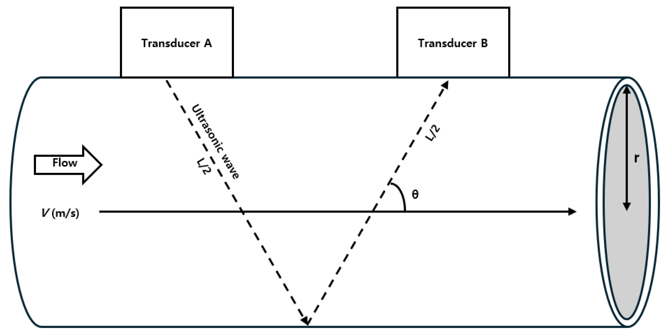
2. Principles and Measurement Model

Figure 1 shows the diagram of the clamp-on ultrasonic flowmeter, illustrating the path of the ultrasonic signals and the placement of the transducers [16,17]. This ultrasonic flowmeter can calculate the flow velocity using the following equation. Here, L represents the length of the path of ultrasonic propagation, v is the velocity of the flow, $\theta$ denotes the angle between the direction of the fluid flow and the propagation of the ultrasonic signal, and c indicates the speed of sound in the fluid.

The ultrasonic signal is first transmitted downstream from transducer A to transducer B, with the propagation time denoted as $t_{BA}$, as follows [18]:

$$t_{BA}={\displaystyle \frac{L}{c-vcos\theta }}$$

(1)

Subsequently, the signal is transmitted upstream from transducer B to transducer A, with the propagation time denoted as $t_{AB}$, as follows:

$$t_{AB}={\displaystyle \frac{L}{c+vcos\theta }}$$

(2)

We define the propagation time difference, $\Delta ToF$, as follows:

$$\Delta \mathit{ToF}=t_{BA}-t_{AB}$$

(3)

The flow velocity follows the following equation:

$$v={\displaystyle \frac{\Delta ToF·c^2}{2·L·cos\theta }}$$

(4)

Using the calculated flow velocity, the flow rate Q can be expressed as follows:

$$Q=K·A·v$$

(5)

where A represents the pipe’s cross-sectional area and K is a calibration factor accounting for flow profiles and sensor characteristics.

3. Proposed Algorithm

This study proposes a low-complexity time-of-flight (ToF) estimation algorithm that combines Hilbert transform-based envelope detection and differentiator-based peak detection in a parallel structure (Algorithm 1). This algorithm focuses on overcoming the limitations of the existing ultrasonic flowmeters in wireless sensor network (WSN) environments where energy efficiency is critical. The Hilbert transform enables accurate envelope extraction [19]. On the other hand, differentiator-based peak detection efficiently identifies the local maximum and minimum values of the signal [20]. Focusing on reducing noise and distortion, this approach enables stable ToF estimation even in energy-sensitive environments. Designed to allow both processes to operate simultaneously through a parallel processing structure, the algorithm significantly increases computational efficiency and stability. At the same time, it is suitable for resource-constrained environments such as WSN by reducing hardware complexity and computational time through selectively handling only the significant peaks within the envelope. This design reduces latency while maintaining high accuracy in noisy and distorted environments, meeting the requirements of real-time ToF estimation.

Algorithm 1: Parallel Peak Detector-Based Envelope Detection

The algorithm works based on two key steps for ToF estimation. First, it extracts an envelope from the input signal and then finds the most critical peak in a specific range to maintain high efficiency and reliability.

In the first step, we compute the input signal’s envelope $x\left[n\right]$, utilizing the Hilbert transform. The Hilbert transform $H\left[x\right[n\left]\right]$ of each signal sample $x\left[n\right]$ is derived from the following expression:

$$H\left[x\left[n\right]\right]={\displaystyle \frac{1}{\pi }}{\int }_{-\infty }^{\infty }{\displaystyle \frac{x\left(\tau \right)}{t-\tau }}d\tau$$

(6)

When the Hilbert transformation is complete, the envelope $E\left[n\right]$ is calculated in the following way:

$$E\left[n\right]=\sqrt{x{\left[n\right]}^2+{\left(H\left[x\left[n\right]\right]\right)}^2}$$

(7)

This allows for the effective extraction of the signal’s amplitude information and a stable representation that mitigates the effects of noise and distortion. The extracted envelope is used as a key factor in peak detection and ToF calculation at a later stage.

The second stage identifies local maxima and minima using a differentiator-based peak detection method. The difference between the consecutive signal values is calculated as follows:

$$x^{\prime }\left[n\right]=x\left[n\right]-x[n-1]$$

(8)

A local maximum is detected when the following conditions are achieved:

$$x^{\prime }[n-1]>0\mathrm{and}{x}^{\prime }\left[n\right]\le 0$$

(9)

Similarly, a local minimum is detected when the following conditions are achieved:

$$x^{\prime }[n-1]<0\mathrm{and}{x}^{\prime }\left[n\right]\ge 0$$

(10)

The detected peak index stores the maximum and minimum values in a separate register to track the peak accurately. This step provides the basis for identifying the most significant peaks within a valid signal range, which the algorithm determines in parallel. This range is centered around the sample with a maximum envelope value $E_{\max \_\mathrm{index}}$, within the $\pm 1$-cycle range $E_{\mathrm{range}}$. It includes samples. The most significant peak, $P_{\mathrm{selected}}$, is the highest peak value within this range. As a result, only the most essential peaks within the signal are selected, reducing noise impact and computational effort. The algorithm returns $P_{\mathrm{selected}}$ as the detected peak, which is used as a key factor for ToF estimation. The proposed method efficiently and systematically combines the envelope and the differentiator-based peak detection to provide a stable and reliable performance even in noisy environments. The two-stage approach reduces computational complexity, making it suitable for resource-constrained systems like wireless sensor networks.

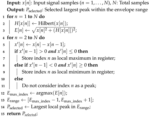
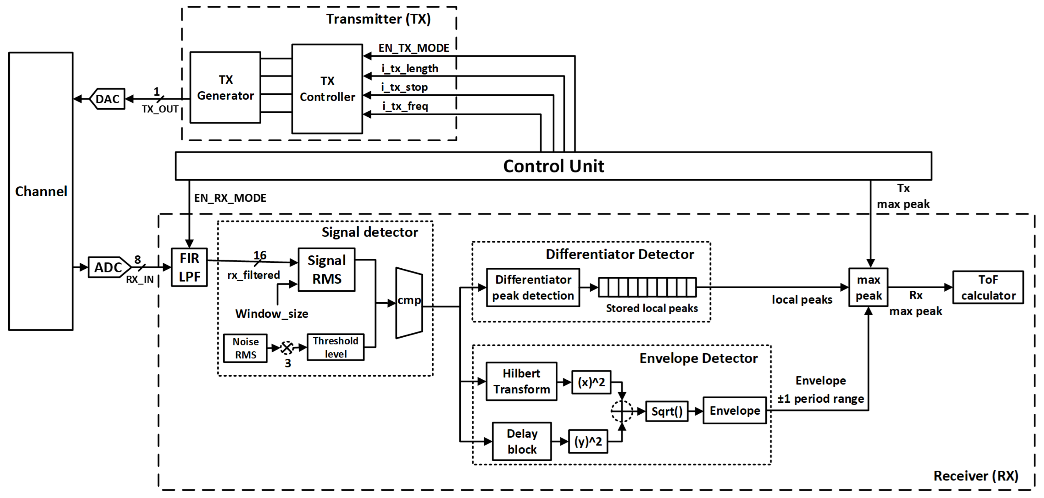
4. System Architecture

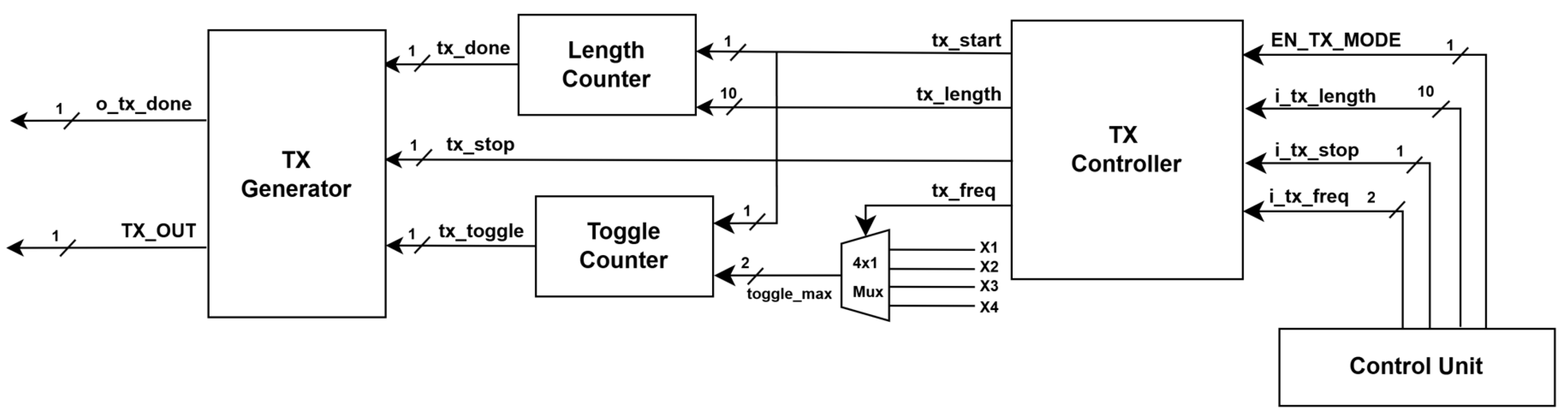
Figure 2 shows the block diagram of the proposed ultrasonic flowmeter system. The system consists of the following two main components: a transmitter and a receiver. The transmitter generates digital signals using a TX Generator and TX Controller. Then, it converts the digital signals into analog signals through a Digital-to-Analog converter (DAC) for transmission via the channel. The receiver captures the analog signals from the channel and converts them into digital signals using an Analog-to-Digital converter (ADC). The receiver pre-processes the received digital signals and estimates the ToF using digital signal-processing algorithms.

4.1. Transmitter

The transmitter in the system is responsible for generating and transmitting ultrasonic signals. Figure 3 shows the block diagram of the transmitter. It consists of a TX controller and a TX generator.

The TX controller is activated by an external control signal EN_TX_MODE and manages the transmission’s start tx_start and termination tx_stop signals. In addition, the TX controller provides the tx_length and tx_freq signals, which control the transducer’s frequency and transmission length through counters. The toggle counter adjusts the toggle count of the transmitter based on the set frequency, while the transmission length counter tracks the number of bits transmitted. Once the preset transmission length is reached, the transmission is terminated. The TX generator receives control signals and counter outputs from the TX controller to generate digital ultrasonic signals. These signals are converted into actual analog ultrasonic signals via a digital-to-analog converter (DAC) and transmitted. The transmitted signal is represented as a sine wave modulated using Gaussian pulses, and the equation is as follows:

$$s\left(t\right)=exp\left(-{\left(f_0·(t-3·T_0)\right)}^2\right)·sin({\omega }_0·t)$$

(11)

where $f_0$ is the central frequency, $T_0$ is the period, and ${\omega }_0$ is the angular frequency. The design of the transmitter enables precise frequency generation and flexible signal control, resulting in an effective response to various flow measurement conditions. To achieve this, the TX controller utilizes parameter registers to configure control signals dynamically. The primary control signals include EN_TX_MODE, i_TX_STOP, i_TX_LENGTH, and i_TX_FREQ. Specifically, EN_TX_MODE reduces energy consumption by making it active only on transmission. In addition, i_TX_STOP allows for precise control by permitting an immediate shutdown when it wants to stop transmission. i_TX_LENGTH reduces unnecessary signal output by dynamically adjusting the length of the transmission signal. Meanwhile, i_TX_FREQ allows for real-time adjustments of the transmission frequency to generate signals suited to the characteristics of the ultrasonic sensor. This allows for the selective utilization of sensors that operate optimally within specific frequency ranges. This design supports various flow measurement conditions in wireless sensor network (WSN) environments and reduces energy consumption, making it suitable for resource-constrained WSN applications.

4.2. Receiver

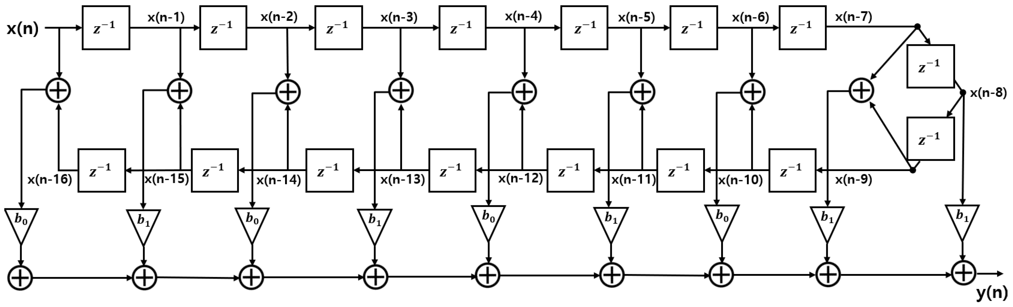
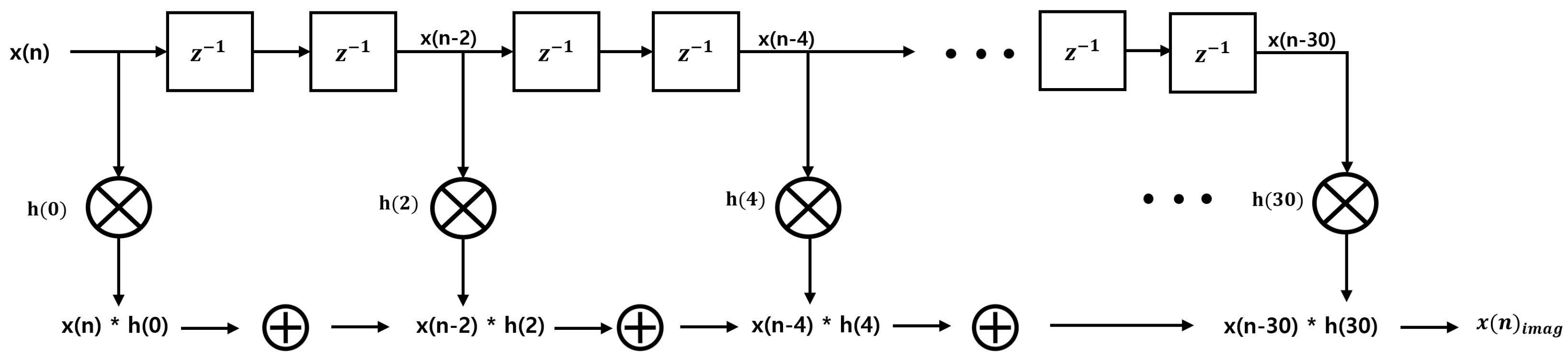
4.2.1. Pre-Processing

The signal received may be affected by high-frequency noise and electromagnetic interference during propagation through the medium. This system employs a digital low-pass filter (LPF) to mitigate these effects. The LPF allows only low-frequency signals below a cut-off frequency of 2.5 MHz to pass and is implemented based on a 17-tap FIR filter. Figure 4 shows the VLSI architecture of the 17-tap LPF, designed for efficient hardware implementation in this system [21]. Utilizing a symmetric structure reduces the number of multipliers by half, lowering the hardware complexity. Furthermore, the LPF maintains a fixed cutoff frequency, ensuring that the filter’s design complexity does not increase even when the frequency of the transmitted signal changes.

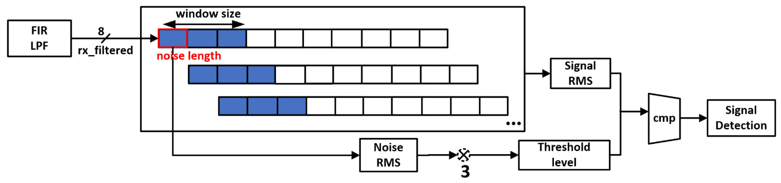
4.2.2. Power Detection Based on Windowing Method

After pre-processing with the low-pass filter (LPF) to reduce noise and interference, the next step involves detecting the presence of the signal received. In this system, a windowing-based power detection method is applied to determine the presence of the signal received [22]. Figure 5 illustrates the windowing-based power detection process. The received signal is sequentially input sample by sample through a shift register. After storing samples equal to the defined window size, the energy within that interval is calculated to detect the signal.

The energy calculation is performed based on the root mean square (RMS), and the energy of the samples within the window size is defined as follows [23]:

$$rx\_rms\left(i\right)=\sqrt{{\displaystyle \frac{1}{W}}\sum _{j=0}^{W-1}rx\_adc{[i+j]}^2}$$

(12)

where $rx\_adc\left[i\right]$ represents the input samples within the window, and W represents the length of the window. As a result of analyzing the waveform characteristics of the transmitted signal, it was observed that the amplitude was low in the 1–2-cycle section, making it difficult to distinguish it from noise. At the same time, the energy was concentrated in the 3-cycle interval, making it the most suitable for signal detection.

The window size is set according to the number of samples in the 3-cycle interval to maximize signal detection performance. The window size is calculated as follows:

$$N_{\mathrm{window}}=3·N_{\mathrm{period}}$$

(13)

where $N_{\mathrm{period}}$ is the number of samples per cycle of the transmitted signal, defined by the period $T_0$ and the sampling interval $T_s$.

$$N_{\mathrm{period}}={\displaystyle \frac{T_0}{T_s}}$$

(14)

In addition, since the amplitude of the transmitted signal is zero during the initial interval (one cycle), only noise exists in this section. Therefore, the noise RMS is calculated based on this interval. The signal detection threshold is set using the noise RMS value, which is defined as follows [24]:

$$\mathrm{Threshold}=3\times \mathrm{Noise}\mathrm{RMS}$$

(15)

The energy of the input signal is measured and compared to a threshold calculated based on the noise RMS to detect the presence of the signal.

Figure 6 shows the RMS profile of the received signal, with the threshold level on the left and the corresponding waveform received on the right, where the signal detection point is marked with a red asterisk. This approach ensures reliable signal detection even in noisy environments.

4.2.3. Proposed Architecture

Following signal detection, the proposed VLSI architecture utilizes Hilbert transform-based envelope detection and differentiator-based parallel peak detection. This architecture optimizes the previously described algorithm from a hardware implementation perspective, aiming for real-time signal processing with low complexity. To implement the Hilbert transform for envelope extraction, the architecture uses a 31-tap FIR filter, as shown in Figure 7. The FIR filter leverages the symmetry of its coefficients, where $h\left[n\right]=h[N-1-n]$, allowing the architecture to use only half the number of multipliers while maintaining the same performance. This optimization significantly reduces computational complexity and conserves hardware resources.

In parallel, the proposed hardware architecture for the differentiator-based peak detector is shown in Figure 8 [25]. This architecture efficiently identifies the local maxima and minima by processing the input signal samples sequentially. It is suitable for environments with limited resources as it is lightweight due to the low use of hardware resources such as comparators, latches, and D flip-flops. Each sample is compared to the previous sample to determine whether it is a local maximum or minimum, and the results are stored in the latch to ensure accuracy. D flip-flops align input signal samples to the clock to ensure stable sequential processing and reduce hardware complexity for real-time signal analysis. Parallel design can simultaneously perform envelope extraction and peak detection, improving the efficiency and real-time performance of the time-of-flight (ToF) estimation system and minimizing computational load.

The selected peak $P_{\mathrm{selected}}$ represents the point with the highest energy among the detected peaks in the valid region. This peak is then used for the ToF estimation. By combining the differentiator’s and the envelope’s valid ranges, the proposed method achieves robust and accurate ToF estimation, even in noisy or attenuated signal environments. This approach also minimizes computational overhead by focusing only on the most significant features of the signal.

5. Results and Discussion

5.1. Simulation Experiment Setup

The performance of the proposed system was validated through LPG simulations conducted using the MATLAB software. The transmitted signal is defined in Equation (11), where the center frequency of the transmitted signal is set to 2 MHz, and the sampling frequency is set to 50 MHz. The propagation time difference is defined in Equation (3), and the flow velocity is calculated using Equation (4). In these equations, c denotes the speed of sound, which is 200 m/s. The ultrasonic path length L is calculated as $D/sin\theta$, and the angle $\theta$ is set to 45°. The pipe has a diameter D of 80 mm and a wall thickness of 0.75 mm, resulting in a radius r of 39.25 mm. The z-coordinate is defined from the center of the pipe, where $z=0\mathrm{m}$, to the wall, where $z=\pm 0.03\mathrm{m}$. The fluid flow conditions were simulated to define the flow velocity distribution and calculate the Reynolds number (Re) using the following equation [26]:

$$\mathrm{Re}={\displaystyle \frac{\rho ·V·D}{\mu }}$$

where $\rho =2.35{\mathrm{kg}/\mathrm{m}}^3$ is the density of LPG, V is the fluid velocity ranging from $0.1\mathrm{m}/\mathrm{s}$ to $1.7\mathrm{m}/\mathrm{s}$, and $\mu =9.5\times {10}^{-6}\mathrm{Pa}·\mathrm{s}$ is the dynamic viscosity of LPG. The Re for each velocity point was then used to classify the flow regime as laminar or turbulent.

Table 1. Background flow in two fluid states based on Reynolds number.

Fluid Velocity (m/s)	Reynolds Number (Re)	Flow Regime
0.10	1979	Laminar
0.30	5937	Turbulent
0.50	9895	Turbulent
0.70	13,853	Turbulent
0.90	17,811	Turbulent
1.10	21,768	Turbulent
1.30	25,726	Turbulent
1.50	29,684	Turbulent
1.70	33,642	Turbulent

provides the Re and flow regimes corresponding to each velocity point in the simulation. As shown, flow is classified as laminar at $0.1\mathrm{m}/\mathrm{s}$ and transitions to turbulent at higher velocities. In the laminar flows, the velocity profile follows a parabolic distribution as follows:

$$v\left(z\right)=v_{\max }·\left(1-{\left({\displaystyle \frac{z}{r}}\right)}^2\right)$$

where $v_{\max }$ represents the maximum flow velocity and is set to 1.7 m/s. For turbulent flows, the velocity profile follows the 1/7 power law as follows:

$$v\left(z\right)=v_{\max }·{\left(1-\left|{\displaystyle \frac{z}{r}}\right|\right)}^{1/7}$$

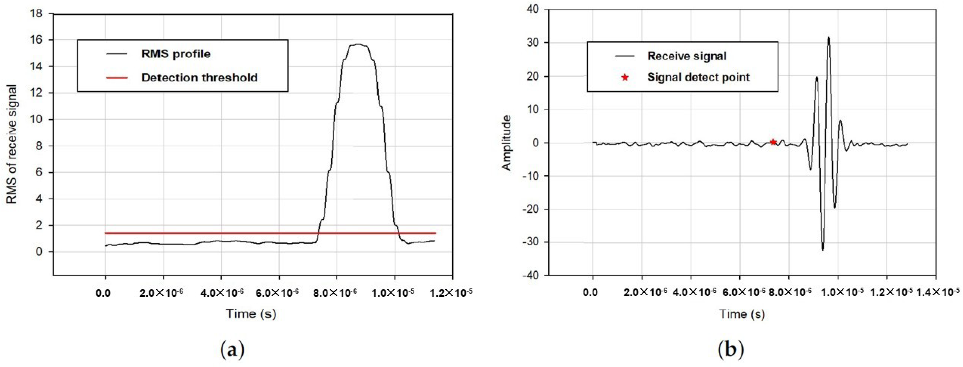
5.2. Performance of the Proposed Method

The efficiency of the proposed algorithm was analyzed within a flow velocity range of 0.1 to 1.7 m/s. For each velocity point, the system calculated the relative deviation using the following formula:

$$\mathrm{Relative}\mathrm{Deviation}(\%)={\displaystyle \frac{\mathrm{Actual}\mathrm{Velocity}-\mathrm{Velocity}\mathrm{Point}}{\mathrm{Velocity}\mathrm{Point}}}\times 100$$

Table 2. Performance of the proposed method based on velocity point, relative deviation, and Reynolds number.

Velocity Point (m/s)	Detected Velocities (m/s)	Relative Deviation (%)	Reynolds Number (Re)	Flow Type
0.10	0.0850	−15.00	1979	Laminar
0.30	0.2750	−8.33	5937	Turbulent
0.50	0.4758	−4.83	9895	Turbulent
0.70	0.6738	−3.75	13,853	Turbulent
0.90	0.8740	−2.89	17,811	Turbulent
1.10	1.0740	−2.36	21,768	Turbulent
1.30	1.2750	−1.92	25,726	Turbulent
1.50	1.4770	−1.53	29,684	Turbulent
1.70	1.6750	−1.47	33,642	Turbulent

summarizes the simulation results. Weak signal strength in the low-velocity region at $0.1\mathrm{m}/\mathrm{s}$ was caused by attenuation [27]. This resulted in a high relative deviation of $-15.00\%$. As the flow velocity increased, the transition to turbulent flow improved signal strength and stability. This reduced the relative deviation to $-1.53\%$ and $-1.47\%$ in the high-velocity region from $1.5\mathrm{m}/\mathrm{s}$ to $1.7\mathrm{m}/\mathrm{s}$. The proposed algorithm demonstrated consistent accuracy in turbulent conditions, where increased flow velocity improved signal strength and stability. The uniformity of the velocity profile further supported this. The method achieved reliable time-of-flight (ToF) estimation in diverse flow conditions.

5.3. Comparison of Performance and Hardware Complexity with Other Methods

The hardware complexity and performance of the proposed method were evaluated based on the relative deviation (%), the number of multipliers (Mul), and the number of adders (Add).

Table 3. Comparisons with other methods: computational complexity and mean relative deviation (N: number of samples).

Method	Signal Processing	Complexity		Mean Relative Deviation (%)
		Mul	Add
Proposed	Signal Detector	75	74	5.07
	17-tap FIR LPF	9	17
	31-tap FIR Hilbert	16	15
	Differentiator Peak Detector	0	0
	Total	305	309
FFT-based correlator [28]	Total	1445	1319	3.47
Multiple zero-crossing detection [29]	DC Removal	0	251	11.67
	Zero-Crossing	0	0
	Energy Calculation	212	106
	Frequency Normalization	106	106
	Energy Normalization	106	106
	Probability Calculation	106	0
	Total	530	569
Dynamic weighted average filter [30]	Weighted Recursive Filter	882	756	3.12
	Dynamic Threshold	0	126
	Total	882	882

summarizes the results of the comparison with the methods proposed by other researchers. For a fair comparison, the performance of the proposed and comparative methods was evaluated in the same velocity range. Additionally, simulation parameters such as transmitted signal characteristics, flow profiles, and attenuation were standardized under identical conditions. The proposed method, with an average relative deviation of 5.07%, demonstrated high accuracy while achieving low complexity, requiring only 305 multiplications and 309 additions. The FFT-based correlator method achieved the lowest mean relative deviation of 3.47% [28]. However, it required the highest hardware complexity, with 1445 multiplications and 1319 additions due to computationally intensive FFT operations. This makes it unsuitable for energy-sensitive environments. The multiple zero-crossing method showed the highest average relative deviation of 11.67%, low detection accuracy, and was sensitive to noise [29]. Additionally, this method required 530 multiplications and 569 additions, which include operations such as energy computation and normalization, further hindering its real-time processing efficiency. The dynamic weighted average filter method demonstrated excellent precision, with an average relative deviation of 3.12% [30]. However, due to the complex filter structure, the multiplication and addition operations had to be performed 882 times each, which significantly burdened energy efficiency. The proposed algorithm combines envelope detection utilizing Hilbert transform-based envelope detection and differentiator-based peak detection to reduce computational complexity while maintaining excellent accuracy. Notably, differentiator-based peak detection can significantly reduce hardware resources because there are no multiplication operations. In addition, the parallel structure enables real-time processing and makes the method suitable for energy-efficient applications like wireless sensor networks (WSNs).

6. Conclusions

This study proposes a low-complexity signal processing approach to the time-of-flight (ToF) estimation suitable for resource-constrained environments such as wireless sensor networks (WSNs). The proposed method demonstrated a structure that can increase computational efficiency while maintaining performance by combining Hilbert transform-based envelope detection and differentiator-based peak detection. The algorithm showed competitive accuracy with a mean relative deviation of 5.07% while significantly reducing hardware complexity, requiring only 305 multiplication and 309 addition operations. These results highlight its suitability for energy-efficient real-time applications, enabling reliable flow measurement with reduced power consumption and extended battery life in sensor networks. Furthermore, the ultrasonic flowmeter’s measurable flow rate range is between $4.11\times {10}^{-4}{\mathrm{m}}^3/\mathrm{s}$ and $8.11\times {10}^{-3}{\mathrm{m}}^3/\mathrm{s}$. This range is calculated using Equation (5) based on the measured flow velocity points, where K is set to one. This result highlights the flowmeter’s capability to effectively measure flow rates within this range, ensuring its adaptability to various industrial and environmental applications. Future research will implement the proposed algorithm on the FPGA platform to verify real-time performance and review its applicability in different operating environments, such as intelligent water resource networks and industrial monitoring systems. These studies will further enhance the algorithm’s practicality and contribute to developing a robust and practical framework for next-generation flow measurement.

References

1. Priyadarshi, R. Energy-efficient routing in wireless sensor networks: A meta-heuristic and artificial intelligence-based approach: A comprehensive review. Arch. Comput. Methods Eng. 2024, 31, 2109–2137. [Google Scholar] [CrossRef]
2. Karthick Raghunath, K.; Koti, M.S.; Sivakami, R.; Vinoth Kumar, V.; NagaJyothi, G.; Muthukumaran, V. Utilization of IoT-assisted computational strategies in wireless sensor networks for smart infrastructure management. Int. J. Syst. Assur. Eng. Manag. 2024, 15, 28–34. [Google Scholar] [CrossRef]
3. Sivakumar, S.; Logeshwaran, J.; Kannadasan, R.; Faheem, M.; Ravikumar, D. A novel energy optimization framework to enhance the performance of sensor nodes in Industry 4.0. Energy Sci. Eng. 2024, 12, 835–859. [Google Scholar] [CrossRef]
4. Khernane, S.; Bouam, S.; Arar, C. Renewable Energy Harvesting for Wireless Sensor Networks in Precision Agriculture. Int. J. Networked Distrib. Comput. 2024, 12, 8–16. [Google Scholar] [CrossRef]
5. Mitra, S.; Chakraborty, B.; Mitra, P. Smart meter data analytics applications for secure, reliable and robust grid system: Survey and future directions. Energy 2024, 289, 129920. [Google Scholar] [CrossRef]
6. Ferrigno, L.A.; Morello, R.; Paciello, V.; Pietrosanto, A. Remote metering in public networks. Metrol. Meas. Syst. 2013, 20, 705–714. [Google Scholar] [CrossRef]
7. Matani, A.G. Internet of things (IoT) in renewable energy utilities towards enhanced energy optimization. In Deregulated Electricity Structures and Smart Grids; CRC Press: Boca Raton, FL, USA, 2022; pp. 113–123. [Google Scholar]
8. Lozano, D.; Mateos, L. Field evaluation of ultrasonic flowmeters for measuring water discharge in irrigation canals. Irrig. Drain. 2009, 58, 189–198. [Google Scholar] [CrossRef]
9. Chen, Q.; Li, W.; Wu, J. Realization of a multipath ultrasonic gas flowmeter based on transit-time technique. Ultrasonics 2014, 54, 285–290. [Google Scholar] [CrossRef] [PubMed]
10. Kaga, Y.; Johguchi, K. A 180 nm CMOS smart ultrasonic water flow meter circuit for IoT smart society. Jpn. J. Appl. Phys. 2021, 60, SBBL05. [Google Scholar] [CrossRef]
11. Rajita, G.; Mandal, N. Review on transit time ultrasonic flowmeter. In Proceedings of the 2016 2nd International Conference on Control, Instrumentation, Energy & Communication (CIEC), Kolkata, India, 28–30 January 2016; IEEE: Piscataway, NJ, USA, 2016; pp. 88–92. [Google Scholar]
12. Munasinghe, N.; Paul, G. Ultrasonic-based sensor fusion approach to measure flow rate in partially filled pipes. IEEE Sens. J. 2020, 20, 6083–6090. [Google Scholar] [CrossRef]
13. Bourke, P. Cross Correlation. Cross Correlation”, Auto Correlation—2D Pattern Identification. 1996. Available online: https://paulbourke.net/miscellaneous/correlate/ (accessed on 28 December 2024).
14. Hsue, S.Z.; Soliman, S.S. Automatic modulation classification using zero crossing. IEE Proc. F Radar Signal Process. 1990, 137, 459–464. [Google Scholar] [CrossRef]
15. Law, T. Elementary signal detection and threshold theory. In Stevens’ Handbook of Experimental Psychology and Cognitive Neuroscience, Methodology; Wiley: Hoboken, NJ, USA, 2018; Volume 5, p. 161. [Google Scholar]
16. Han, J.; Liu, H.; Zhou, Y.; Zhang, R.; Li, C. Studies on the transducers of clamp-on transit-time ultrasonic flow meter. In Proceedings of the 2014 4th IEEE International Conference on Information Science and Technology, Shenzhen, China, 26–28 April 2014; IEEE: Piscataway, NJ, USA, 2014; pp. 180–183. [Google Scholar]
17. Afandi, A.; Khasani; Deendarlianto; Catrawedarma, I.G.N.B.; Wijayanta, S. The development of the ultrasonic flowmeter sensors for mass flow rate measurement: A comprehensive review. Flow Meas. Instrum. 2024, 97, 102614. [Google Scholar] [CrossRef]
18. Iooss, B.; Lhuillier, C.; Jeanneau, H. Numerical simulation of transit-time ultrasonic flowmeters: Uncertainties due to flow profile and fluid turbulence. Ultrasonics 2002, 40, 1009–1015. [Google Scholar] [CrossRef] [PubMed]
19. Ulrich, T. Envelope Calculation from the Hilbert Transform; Technical Report; Los Alamos National Laboratory: Los Alamos, NM, USA, 2006. [Google Scholar]
20. Kaur, A.; Kumar, S.; Agarwal, A.; Agarwal, R. An efficient R-peak detection using Riesz fractional-order digital differentiator. Circuits Syst. Signal Process. 2020, 39, 1965–1987. [Google Scholar] [CrossRef]
21. Bose, S.; De, A.; Chakrabarti, I. Area-delay-power efficient VLSI architecture of FIR filter for processing seismic signal. IEEE Trans. Circuits Syst. II Express Briefs 2021, 68, 3451–3455. [Google Scholar] [CrossRef]
22. Prabhu, K.M. Window Functions and Their Applications in Signal Processing; Taylor & Francis: Abingdon, UK, 2014. [Google Scholar]
23. Chai, T.; Draxler, R.R. Root mean square error (RMSE) or mean absolute error (MAE). Geosci. Model Dev. Discuss. 2014, 7, 1525–1534. [Google Scholar]
24. Barshan, B. Fast processing techniques for accurate ultrasonic range measurements. Meas. Sci. Technol. 2000, 11, 45. [Google Scholar] [CrossRef]
25. Jordanov, V.T.; Hall, D.L. Digital peak detector with noise threshold. In Proceedings of the 2002 IEEE Nuclear Science Symposium Conference Record, Norfolk, VA, USA, 10–16 November 2002; IEEE: Piscataway, NJ, USA, 2002; Volume 1, pp. 140–142. [Google Scholar]
26. Smits, A.J.; McKeon, B.J.; Marusic, I. High–Reynolds number wall turbulence. Annu. Rev. Fluid Mech. 2011, 43, 353–375. [Google Scholar] [CrossRef]
27. Joshi, S.; Zaitsev, B.; Kuznetsova, I. Miniature high efficiency transducers for use in ultrasonic flow meters. J. Appl. Phys. 2009, 105, 034501. [Google Scholar] [CrossRef]
28. Ren, R.; Wang, H.; Sun, X.; Quan, H. Design and implementation of an ultrasonic flowmeter based on the cross-correlation method. Sensors 2022, 22, 7470. [Google Scholar] [CrossRef] [PubMed]
29. Fang, Z.; Su, R.; Hu, L.; Fu, X. A simple and easy-implemented time-of-flight determination method for liquid ultrasonic flow meters based on ultrasonic signal onset detection and multiple-zero-crossing technique. Measurement 2021, 168, 108398. [Google Scholar] [CrossRef]
30. Zhou, J.; Wang, P.; Wang, R.; Niu, Z.; Zhang, K. Signal processing method of ultrasonic gas flowmeter based on transit-time mathematical characteristics. Measurement 2025, 239, 115485. [Google Scholar] [CrossRef]
Figure 1. Diagram of the clamp-on ultrasonic flowmeter.
Jsan 14 00012 g001
Figure 2. Block diagram of the proposed method.
Jsan 14 00012 g002
Figure 3. Block diagram of the transmitter. The transmitter is activated by EN_TX_MODE, and the output signal is delivered through TX_OUT.
Jsan 14 00012 g003
Figure 4. The 17-tap low-pass FIR filter VLSI architecture.
Jsan 14 00012 g004
Figure 5. Windowing-based power detection process.
Jsan 14 00012 g005
Figure 6. (a) RMS profile of the received signal with threshold level; (b) waveform of the received signal with detection point marked. The system allows the TX controller to adjust the transmission signal frequency f 0 , enabling dynamic window size adjustments.
Jsan 14 00012 g006
Figure 7. The 31-tap Hilbert transform FIR filter VLSI architecture.
Jsan 14 00012 g007
Figure 8. Architecture of the differentiator-based peak detector.
Jsan 14 00012 g008