Article

Helicopters Turboshaft Engines Neural Network Modeling under Sensor Failure

by
Serhii Vladov
1,*,
Anatoliy Sachenko
2,3,*,
Valerii Sokurenko
1,
Oleksandr Muzychuk
1 and
Victoria Vysotska
4,5
1
Kharkiv National University of Internal Affairs, 27, L. Landau Avenue, 61080 Kharkiv, Ukraine
2
Research Institute for intelligent Computer Systems, West Ukrainian National University, 11, Lvivska Street, 46009 Ternopil, Ukraine
3
Department of Teleinformatics, Kazimierz Pulaski University of Radom, 29, Malczewskiego Street, 26-600 Radom, Poland
4
Information Systems and Networks Department, Lviv Polytechnic National University, 12, Bandera Street, 79013 Lviv, Ukraine
5
Institute of Computer Science, Osnabrück University, 1, Friedrich-Janssen-Street, 49076 Osnabrück, Germany
*
Authors to whom correspondence should be addressed.
J. Sens. Actuator Netw. 2024, 13(5), 66; https://doi.org/10.3390/jsan13050066
Submission received: 15 September 2024 / Revised: 7 October 2024 / Accepted: 8 October 2024 / Published: 10 October 2024

Abstract

:
This article discusses the development of an enhanced monitoring and control system for helicopter turboshaft engines during flight operations, leveraging advanced neural network techniques. The research involves a comprehensive mathematical model that effectively simulates various failure scenarios, including single and cascading failure, such as disconnections of gas-generator rotor sensors. The model employs differential equations to incorporate time-varying coefficients and account for external disturbances, ensuring accurate representation of engine behavior under different operational conditions. This study validates the NARX neural network architecture with a backpropagation training algorithm, achieving 99.3% accuracy in fault detection. A comparative analysis of the genetic algorithms indicates that the proposed algorithm outperforms others by 4.19% in accuracy and exhibits superior performance metrics, including a lower loss. Hardware-in-the-loop simulations in Matlab Simulink confirm the effectiveness of the model, showing average errors of 1.04% and 2.58% at 15 °C and 24 °C, respectively, with high precision (0.987), recall (1.0), F1-score (0.993), and an AUC of 0.874. However, the model’s accuracy is sensitive to environmental conditions, and further optimization is needed to improve computational efficiency and generalizability. Future research should focus on enhancing model adaptability and validating performance in real-world scenarios.

1. Introduction

1.1. Relevance of the Research

In modern helicopter operations equipped with turboshaft engines (TEs), ensuring the reliable performance engines under sensor failure conditions is of paramount importance. Sensor failure can significantly impact flight stability and safety, as sensor data is crucial for engine control and condition monitoring [1]. Traditional data processing methods often fall short in detecting anomalies and recovering accurate information, necessitating the use more advanced technologies [2,3]. A promising approach involves neural network modeling of the performance helicopter TE capable of handling sensor signals and restoring lost information [4].
The relevance of developing neural network-based models for helicopter TEs, particularly under sensor failure conditions, lies in the need for enhanced reliability and safe helicopter operations [5]. Neural networks, with their ability to train and adapt, can effectively model complex dynamic processes and provide high accuracy in prediction and anomaly detection [6]. This is especially crucial in scenarios where sensor failure could lead to critical situations, requiring prompt data recovery for real-time decision-making. Thus, the development and implementation of neural network models for processing and recovering data under sensor failure is not only a timely task but essential for ensuring flight safety and extending the operational life of aviation engines.

1.2. State-of-the-Art

Contemporary research on the helicopter TE modeling using neural networks is actively advancing and encompasses a broad range of tasks aimed at improving the aviation systems reliability and safety [7]. A key focus is the development of a model that can predict engine behavior under sensor failure and restore missing data [4]. Machine learning methods, such as recurrent neural networks (RNN) [8,9] and long short-term memory (LSTM) [10,11], have demonstrated high effectiveness in processing time series data and detecting anomalies in engine performance. Currently, research is centered on integrating neural networks with traditional diagnostic and predicting methods [12,13], enabling the creation of hybrid systems that combine the physically strengths-based models and adaptive training algorithms.
Of particular interest is developing autonomous diagnostic and control systems capable of operating under sensor failure without human intervention [14,15]. These systems utilize neural networks trained on extensive datasets and can adapt to changes in engine behavior while responding promptly to emerging issues. Integrating these systems into onboard helicopter control systems requires high reliability and fault tolerance [16]. Additionally, research includes creating models that account for various types of failure and their impact on engine operation, as well as employing generative models and probabilistic graphical approaches to predict rare but critical events [17,18,19].
Recent research also focus on the Internet of Things (IoT) technologies [20] and cloud computing [21] implementation to enhance real-time data collection and analysis about engine conditions. This approach significantly extends the capabilities of neural networks by leveraging distributed computing resources and processing data on remote servers. Such methods make monitoring and control systems more scalable and flexible, which is crucial for large aviation fleets. Thus, contemporary research aims to develop reliable, adaptive, and autonomous systems that not only improve flight safety but extend the operational life of aviation equipment, reducing maintenance and operational costs.
Existing research on modeling helicopter TEs often faces challenges related to accurate prediction of the engine behavior under varying operational conditions and sensor failure. Traditional models [12,13] may struggle with capturing the engines complex, non-linear dynamics, especially when dealing with multivariate time series data and non-stationary environments. These limitations result in the diagnostic and prognostic systems reduced accuracy and reliability. The necessity for employing a neural network autoregressive with exogenous inputs (NARX) model [22,23,24] arises from its capability to handle such complexities by effectively modeling the temporal dependencies and incorporating external influences.
Based on the above, the research aims to develop a helicopter TE neural network model to simulate its parameters in its sensor network for a sensor failure event. The object of the research is the helicopter TE sensor network. The subject of the research includes the helicopter TE sensor network diagnostic methods and means. To achieve this aim, the following scientific and practical tasks were solved:
  • Development of a mathematical model to determine the helicopter TE sensor network output signal in a sensor failure case.
  • Development of a neural network and its training algorithm to model helicopter TE parameters in a sensor network failure event.
  • Development of a test bench for the helicopter TE parameters in a sensor network for the semi-naturalistic modeling implementation of a sensor failure event.
  • Conduct a computational experiment consisting of model helicopter TE parameters during a gas-generator rotor speed sensor failure under various temperature conditions.
  • Assess the results obtained for quality using traditional metrics.
This research main contribution is the development of a helicopter TE sophisticated monitoring and control system using a detailed mathematical model and NARX neural network, achieving a high accuracy in detecting sensor disconnections and effectively simulating various failure scenarios, including single and cascading failure.

1.3. Paper Organization

This paper consists of an introduction, “Materials and Methods”, “Case Study”, and “Discussion” sections, a conclusion, and references. The introduction justifies the relevance behind the research, reviews existing studies, highlights unresolved research issues, and defines the aim, object, and subject behind this study. In the “Materials and Methods” section, a mathematical model was developed for helicopter TE dynamics in a sensor failure event, along with a neural network model that implements this dynamic. The “Case Study” section presents results from the research on the developed neural network model, simulating various types of sensor failure in helicopter TEs. The research included generating a training dataset, preprocessing it, and validating the neural network model on a developed semi-real simulation test bench. The “Discussion” section provides a comparative analysis of the proposed neural network model training algorithm with three types of genetic algorithms, as the closest analogous approach to training such neural networks. The section also outlines the achievements, the results limitations, and the prospects for further research. The conclusion summarize the key research findings.

2. Materials and Methods

The helicopter TE complex model as a control object based on a fundamental model is a component-based nonlinear thermogas-dynamic model [25] which simulates the engine operation in steady-state conditions within the applicable range as follows:
X = f X ¯ , V ¯ , U ¯ , Y = φ X ¯ , V ¯ , U ¯ ,
where X ¯ = n T C , n F T , T G * T is the state variables vector; f and φ are nonlinear operators.
The helicopter TE complex model, regarded as a control object, is based on a nonlinear thermogas-dynamic framework that simulates engine performance under steady-state conditions across a range of operational modes. The model is defined by two key nonlinear relations (1): the state equation X = f X ¯ , V ¯ , U ¯ and the output equation Y = φ X ¯ , V ¯ , U ¯ , where X ¯ represents the state variables, including gas-generator rotor r.p.m., free turbine rotor speed, and gas temperature before the compressor turbine. The dynamic variables V ¯ capture internal processes such as fuel dynamics and thermal inertia, while the control inputs U ¯ include variables like fuel flow rate. These nonlinear operators f and φ describe how the system state and its outputs evolve in response to internal dynamics and control inputs. This model serves as the foundation for understanding engine behavior, facilitating the advanced control and monitoring systems development that account for the helicopter TE nonlinear and time-varying characteristics.
The helicopter TE piecewise-linear model is derived from a fundamental model using a standard method [26]. This model includes the engine starting process, including ignition [27]. The helicopter TE fault scenarios are modeled to address phenomena such as compressor surge, failure to ignite, and flameout [28]. The helicopter TE systems encompass various subsystems, including fuel (pumps, metering units, drives, injector manifolds, and filters), starting (starter, fuel supply system, ignition, gas-generator mechanization, and electrical power), lubrication, bleed air, air, and drainage systems [29]. The references analysis [26,27,28] shows that in-flight monitoring and control models and algorithms involve continuous parameter and signal monitoring, checking allowable limits, engine mode identification, data preparation for ground control and predicting, engine operating time monitoring, diagnostic information processing, and starting control, shutdown, and combustion chamber processes, as well as fault signal generation. These models are designed to handle sensor failure by incorporating fault detection and recovery mechanisms, ensuring that characteristics are aligned across different levels, and maintain operational control even when sensor data is incomplete or unreliable. Representing these characteristics in a criterion-normalized form ensures that engine component models remain accurate and effective within comprehensive monitoring and operational control, including identification based on experimental data [30]. Moreover, the models include specialized algorithms to detect and compensate for sensor failure (Table 1), thereby mitigating their impact on critical flight parameters and maintain the reliability of in-flight engine performance monitoring [31].
The rows in the matrix denote failure modes, while the columns reflect various aspects of the system’s impact potential. The cells in the matrix show the extent or nature of each type of failure and its influence on the system specific aspects [31].
The task for the computer modeling system to address the helicopter TE and system failure is to simulate both single and “cascading” failure. This includes the automatic activation of failure in the engine, its systems, sensors, and actuators in a specified sequence. The dynamics for the helicopter TE and its systems, when simulating the i-th failure, are modeled using the differential equation:
x = (A + ∆iA) ∙ x(t) + (B + ∆iB) ∙ u(t).
The output signal is defined as follows:
x t = 0 t A + Δ i A x t + B + Δ i B u t d t .
The helicopter TE and system failure are simulated by modifying the coefficients in dynamic models. For sudden failure, this involves an abrupt change in coefficient A by ∆A and in coefficient B by ∆B. The magnitude of these changes is predetermined based on the engine and system model for each specific failure. For instance, if a compressor blade breaks, compressor efficiency decreases, which is reflected in corresponding changes to coefficients ∆A and ∆B in the dynamic model. Other types of engine failure, such as combustion chamber burnout or compressor turbine blade destruction, result in different changes to ∆A and ∆B. Failure in the helicopter TE systems is determined similarly within their respective models.
To expand the model significantly, the computer simulation system for the helicopter TE and system failure not only addresses single and “cascading” failure but incorporates time-varying failure, sensor noise, and system interactions, thereby enhancing the accuracy and robustness of the simulation. This model includes the automatic activation of failure in the engine, its systems, sensors, and actuators in a specified sequence, with failure reflecting in both an immediate and delayed effect.
The dynamics for the helicopter TE and its systems, when simulating the i-th failure, are described by the differential equation:
d x t d t = A + Δ i A x t + B + Δ i B u t + ϵ i t .
Here, ΔiA(t) and ΔiB(t) are time-dependent changes in the system matrices due to the i-th failure, and ϵi(t) represents external disturbances or sensor noise, which is modeled as a stochastic process.
The output signal is then defined by:
y t = C 0 t A + Δ i A x τ + B + Δ i B u τ d τ + D u t ,
where C and D are output matrices that may also change with the failure:
C = C0 + ΔiC(t), D = D0 + ΔiD(t).
The helicopter TE and system failure are thus simulated by modifying these coefficients in the dynamic models. For sudden failure, this involves an abrupt change in coefficients A, B, C, and D by their respective Δ values. These changes for magnitude and time course are predetermined based on the detailed engine models and the systems for each specific failure scenario.
For example, in the event of compressor blade breakage, the efficiency decreases, which is expressed in corresponding changes to the coefficients ΔiA(t) and ΔiB(t) in the dynamic model. Additionally, a gradual failure, such as the slow degradation of a fuel pump, are modeled with time-varying coefficients:
ΔiA(t) = ΔiA0 ∙ eλt, ΔiB(t) = ΔiB0 ∙ eλt,
where λ is a failure rate parameter that controls the degradation time scale.
Other types of engine failure, such as combustion chamber burnout or compressor turbine blade destruction, lead to different time-varying changes in ΔiA(t) and ΔiB(t). Failure in the helicopter TE systems, such as those in lubrication or fuel systems, are determined similarly within their respective models, allowing the simulation to capture the failure immediate and assess the long-term effect on overall engine performance.
The expanded model, which simulates helicopter TE and system failure by modifying time-dependent coefficients in dynamic equations, is well-suited for implementation using a neural network autoregressive with exogenous inputs (NARX) architecture. The NARX network excels at capturing the complex temporal dependencies and nonlinear relationships inherent in the dynamic system, allowing for accurate modeling of both sudden and gradual failure. By adjusting its internal weights based on time-series data, the NARX network can seamlessly integrate the time-varying changes in system coefficients, such as ΔiA(t) and ΔiB(t), and effectively simulate the impact of failure across various subsystems. This approach ensures that the model not only captures immediate effects but adapts to long-term degradation processes, making it a robust and easily implementable solution for real-time failure prediction and system monitoring.
The helicopter TE neural network model formation, assumed to be non-linear, is further interpreted as obtaining the helicopter movement original mathematical model neural network approximation, specified in one form or another, most often in the differential equations system form. The error signal ε, which guides the neural network model training, is the difference square between the control object yp and the neural network model ym output, which are under the control signal u influence. The trained neural network model implements a recurrent-type calculation scheme, in which the u values at time ti are used to calculate the output value for time ti+1. As the helicopter TE model is a dynamic object, the nonlinear autoregressive network (NARX type with external inputs) was chosen (Figure 1) as it corresponds to the nature of the engine control task under consideration [22,23,24].
The NARX model is a recurrent dynamic layered neural network model with delay elements at the network inputs and with feedback between layers [32,33]. The NARX model implements a dynamic mapping described by the following form difference equation:
y ^ t = ψ y ^ t 1 , y ^ t 2 , , y ^ t N y , u t 1 , u t 2 , , u t N u ,
where the output signal value y ^ t for a given time t is calculated based on the values y ^ t 1 , y ^ t 2 , , y ^ t N y of this signal for the previous time points sequence, as well as the input (control) signal values u t 1 , u t 2 , , u t N u external to the NARX model. In the general case, the history length for outputs and controls may not coincide, that is, N y N u .
Since the NARX network provides the greatest accuracy for solving identification problems [34], this network is chosen to solve the problem posed in the research. According to [35], the NARX model is presented in the form:
y j 1 n = f 1 b j 1 + i = 1 M 0 w i j 1 n i 1 + i = M 0 + 1 M 0 + M 1 y 2 n i ,   j 1 , N 1 ¯ ,
y 2 n = f 2 b 2 + i = 1 N 1 w i 2 y i 1 n ,
where N(k) is the neurons number in the k-th layer; M(k) is the delay in the k-th layer; w i j 1 n is the connection weight from a neuron at time n – (i – 1) to the j-th neuron in the first layer at time n; w i 2 n is the connection weight from the i-th neuron to the neuron in the second layer at time n; y j 1 n is the output weight the j-th neuron in the first layer; y(2)(n) is the neuron output in the second layer; f(k) is the neurons activation function of the k-th layer (logistic or hyperbolic tangent).
In this research, to train the model, a model adequacy criterion was chosen, which means choosing the parameters w i j 1 n and w i 2 n such values that provide the mean square error minimum (the difference between the output according to the model and the desired output):
F = 1 P p = 1 P y p d p 2 min w i j 1 , w i 2 ,
where P is the test implementations number; yp is the result obtained from the model; dp is the desired result.
Training the neural network model (9)–(11) is subject to criterion (11), for which a training algorithm based on the backpropagation algorithm is proposed [35]. Training iteration number n = 1, y 1 n i = 0 , i 1 , N 1 ¯ , initialization of all biases (thresholds) b j k n and network weights in layers w i j 1 n , i 1 , M 0 + M 1 ¯ , j 1 , N 1 ¯ , i 1 , N 1 ¯ , where N(1) is the neuron number in the first layer, M(k) is the delay in the k-th layer. The training set is specified x , d x μ R ,    d μ R , μ 1 , P ¯ , where xμ is the μ-th factors vector, dμ is the desired responses μ-th vector, P is the training set power. The current pair number from the training set is μ = 1. Calculate the output signal for each layer (forward stroke):
y 0 n i 1 = x μ i 1 ,   i 1 , M 0 ¯ ,   y j 1 n = f 1 s j 1 n ,   j 1 , N 1 ¯ , s j 1 n = i = 0 M 0 w i j 1 n y 0 n i 1 + i = M 0 + 1 M 0 + M 1 w i j 1 n y 2 n i , y 2 n = f 2 s 2 n , s 2 n = i = 0 N 1 w i 2 n y i 1 n .
It is believed that
w 0 j 1 n = b j 1 n , w 0 2 n = b 1 n , y 0 n = y 0 1 n = 1
.
The neural network results mean square error calculation:
E n = 1 2 e 2 n , e n = y 2 n d μ .
Setting up synaptic weights (reverse). To adjust the weighting coefficients, a recursive algorithm is used, which is first applied to the neural network output neurons, and then traverses the network in the opposite direction to the first layer. Synaptic weights are adjusted according to the expression:
w i j 1 n + 1 = w i j 1 n η E n w i j 1 n ,   w i j 2 n + 1 = w i j 2 n η E n w i 2 n ,
where η is the parameter that determines the training rate (with large η, training occurs faster, but the danger of obtaining an incorrect solution increases), 0 < η < 1. Then:
E n w i 2 n = y i 1 n g 2 n , E n w i j 1 n = y 2 n i g j 1 n ,   if   i > M 0   y 2 n i 1 g j 1 n ,   if   i M 0 g 2 n = f 2 s 2 n y 2 n d μ , g j 1 n = f 1 s j 1 n w j 2 n g 2 n .
Checking the termination condition. If the next training epoch is not completed, increase the iteration counter by 1 and move on to the next training example. If the next training epoch is completed and the average training error exceeds the specified threshold, then a new training epoch begins. And finally, if the next training epoch is completed and the average training error is less than a specified threshold, then training is completed.
An alternative to the backpropagation algorithm is the genetic algorithm. The weight vector is used as an individual in the genetic algorithm, and criterion (11) is used as the fitness function.
To enhance the NARX neural network robustness to sensor failure, several corrective mechanisms were integrated into the training algorithm.
When a sensor fails, omitting the data instead, interpolation or extrapolation methods can be used to restore missing values. Let x(t) represent the input data vector at time t, and xi(t) denote data from sensor i (where i is the failed sensor index). The following expression can be used for interpolation:
x ^ i t = 1 n j = 1 n x i t Δ t j ,
where Δtj represents the time intervals over which data from other sensors were collected.
If the output data from a sensor are incomplete or erroneous, weights in the neural network can be adjusted to reduce the impact of this data on training. The weight update expression is:
w n e w = w o l d η δ x t ,
where η represents the training rate, δ is the error (difference between predicted and actual values), and x(t) represents the input data.
To improve robustness to sensor failure, regularization techniques can be employed to penalize large weights. The regularization equation can be expressed as:
L w = 1 2 i λ i w i 2 ,
where λi represents the regularization coefficient for weight wi. This regularization helps the erroneous data influence to diminish by encouraging reliance on more reliable features.
During prediction, if data from some sensors is missing, a model can estimate probable values. The expression for estimating missing data is:
x ^ i t = ϕ x a v a i l a b l e t ,
where ϕ is a function based on available data that predicts values for the missing input data xavailable(t). The pseudocode of the NARX neural network (Figure 1) training is presented in Algorithm 1.
Algorithm 1: The pseudocode of the NARX neural network training (author’s research).
initialize_weights();
learning_rate = 0.01;
epochs = 1000;
N = length_of_training_data;
d_in = input_delay;
d_out = output_delay;
for epoch in range(epochs):
  total_error = 0;
  for i in range(d_in, N):
  x = get_input_sequence(i, d_in);
  y_true = get_true_output(i);
  y_pred = forward_pass(x);
  error = y_true − y_pred;
  total_error += error ** 2;
  gradients = backward_pass(error, x);
  update_weights(gradients, learning_rate);
print(f“Epoch {epoch + 1}, Total Error: {total_error}”);
if total_error < threshold:
  break.

3. Case Study

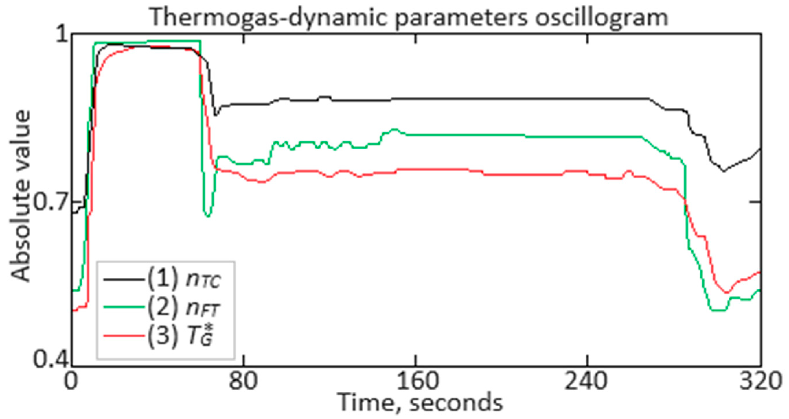
The research object in this work is the TV3-117 turboshaft engine, which serves as the powerplant for the Mi-8MTV helicopter and its various modifications. This engine is extensively utilized in both civil and military aviation [36,37,38]. Parameters recorded on board the helicopter are: T G * (t) is the gas temperature in front of the compressor turbine (a sensor consisting of 14 T-101 thermocouples is used), nTC(t) is the gas-generator rotor r.p.m. (a D-2M sensor is used), and nFT(t) is the free turbine rotor speed (a D-1M sensor is used). During the NARX neural network training, output data were recorded during the TV3-117 TE flight tests aboard the Mi-8MTV helicopter using the onboard control system. Data were collected was over a 320-s interval of an actual flight with a sampling period of 1 s.
Figure 2 illustrates an increase in the parameter values from 20 to 65 s by approximately 1.5 to 1.8 times, attributed to the engine’s transient operating mode. As noted in the introduction, the engine operates in steady state conditions about 85% of the time, while approximately 15% is spent in transient conditions. The values for nTC, nFT, T G * 256 were selected according to Figure 2 (Table 2). This dataset amount is justified by its ability to cover sufficient variations in the helicopter TE parameters, enabling the NARX neural network to effectively train and accurately identify the engine’s dynamic model under flight conditions. Additionally, a sample size of 256 is adequate to ensure normal distribution, which is essential for the statistical significance and reliability of the training set in the neural network for identifying the dynamic model of the helicopter TE.
To effectively construct the training dataset for the NARX neural network, a systematic approach is required to extract the relevant parameter values from the recorded data. This involves selecting 256 data points, which correspond to specific timestamps during the flight tests, ensuring a comprehensive representation of the engine’s operational characteristics. The following pseudocode (Algorithm 2) outlines the process for obtaining this training sample from the gathered parameter values.
Algorithm 2: The pseudocode describing how the sample sizes for the training and test datasets were obtained (author’s research).
sensor_data = get_sensor_data();
length = len(sensor_data);
sample_size = 256;
def get_training_sample(sensor_data, sample_size):
  if length < sample_size:
    raise ValueError(“Data are insufficient to obtain a dataset”);
  training_sample = [];
  for i in range(sample_size):
    index = select_index(length);
    training_sample.append(sensor_data[index]);
  return training_sample;
training_sample = get_training_sample(sensor_data, sample_size);
normalized_sample = normalize(training_sample);
train_model(normalized_sample).
To assess the training dataset homogeneity, the value χ2 = 24.918 is calculated according to [39], which is below the critical value χ c r i t i c a l 2 = 27.683 for df = 13 degrees of freedom at a significance level of α = 0.01. This indicates homogeneity based on the Fisher–Pearson criterion. To confirm this further, the N = 256 training sample is split into two equal subsamples of n1 = n2 = 128 elements each. According to [40], the value F = 5.573 is obtained, which is below the critical value Fcritical = 5.74. This confirms the homogeneity of the training set based on the Fisher–Snedecor criterion.
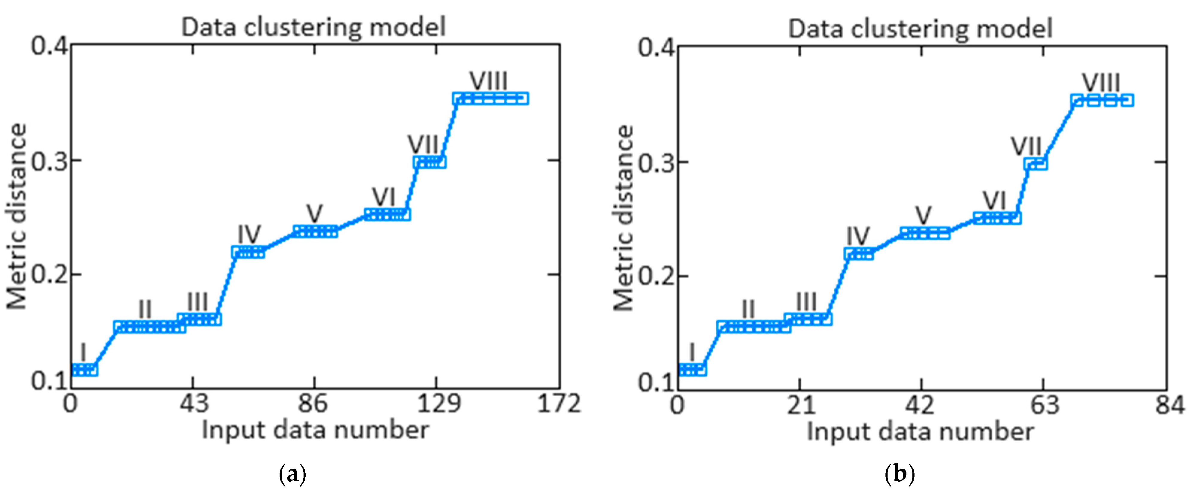
The representativeness of the training and test datasets were evaluated using cluster analysis, aimed at partitioning the input dataset x = (nTC, nFT, T G * ) (Table 2) into k distinct clusters, where k is predefined. Each cluster groups objects that are more similar to one another than to those in other clusters. The k-means method was employed, which minimizes the squared distances between objects and cluster centroids sum. Each object xi is assigned to the nearest centroid based on C i = arg min j x i μ j 2 , where μj represents initial centroids and x i μ j 2 is the Euclidean distance between xi and μj. Centroids are then recalculated as the average of objects within each cluster using μ j = 1 C j x i C j x i , where ∣Cj∣ denotes the object number in the j-th cluster. This process is repeated until centroid changes are minimal, or a specified number of iterations is reached [41,42]. The training data (Table 2) cluster analysis identified eight clusters (I–VIII). Following random selection, training and test samples were created in a 2:1 ratio (67 and 33%, respectively). Analysis of both datasets showed the presence of eight clusters in each, indicating a similar composition. The distances between clusters were nearly identical in both samples, confirming their similarity (Figure 3). Thus, the optimal sample sizes were determined as follows: training dataset is 256 elements (100%), control dataset is 172 elements (67% of the training dataset), and test dataset is 84 elements (33% of the training dataset).
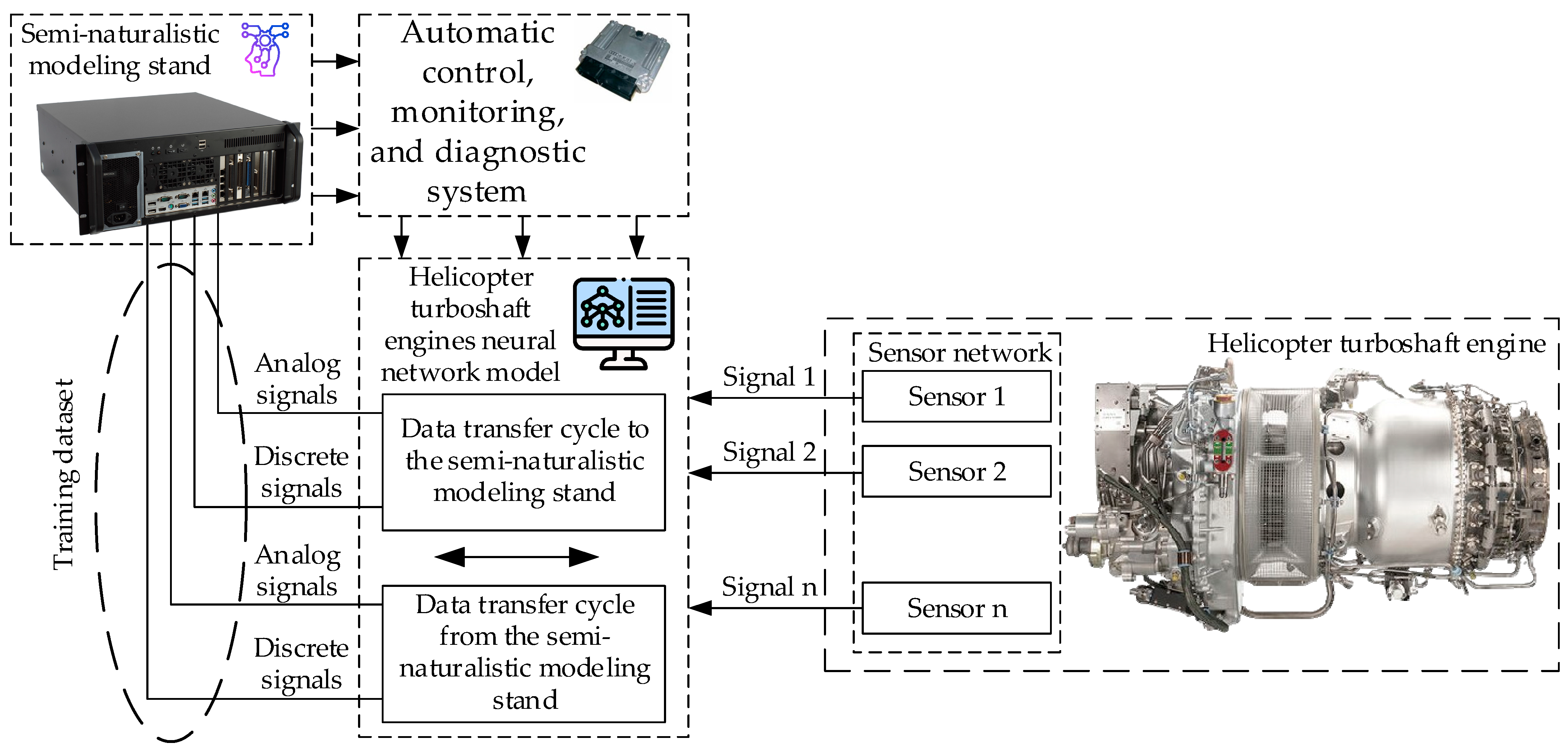
This study involved a computational experiment utilizing a developed semi-physical modeling (SPM) stand. The SPM stand is designed for the helicopter TE parameters real-time simulation, modeling the helicopter TE operating modes across various flight altitudes and speeds, interacting with higher-level systems through communication channels, and verifying the automatic control, monitoring, and diagnostic systems (ACMDS), among other tasks [43,44]. Figure 4 illustrates the interaction scheme between the helicopter TE neural network model and the SPM stand. The neural network model is divided into two-time cycles, each executed on the personal computer’s central processor separate core. The primary cycle, with the highest priority, handles data reception from the SPM stand and neural network operations. The secondary cycle, with lower priority, controls the transfer of computed model data to the SPM stand. This division into two-time cycles with different priorities is essential for ensuring real-time operation of the model. The SPM stand operates within the Matlab Simulink graphical simulation environment, which includes communication channels, a fuel injector emulator, visualization systems, recording, and other components (Figure 5). Integration of the trained helicopter TE neural network model into the Simulink format is achieved using built-in tools, which makes this procedure straightforward, justifying the choice of this package for model implementation.
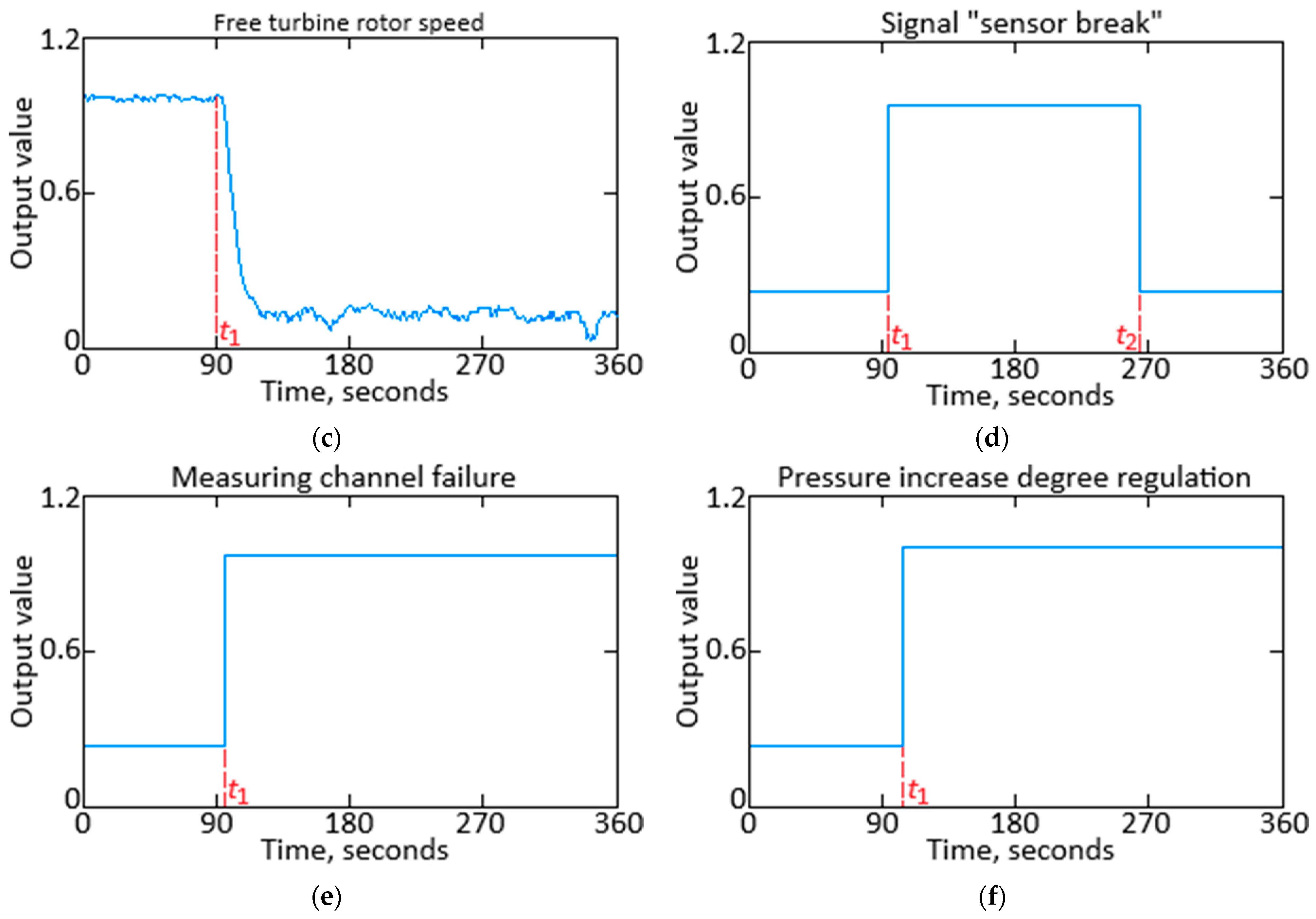
To verify the model physically is simulated in the sensor simulator output electrical circuit executive system, break, and short circuit. The logic for switching keys to simulate sensor failure, actuators and the engine is set by the operator using k(n + 6) signs in a software-controlled dial field [43,45,46,47]. When the gas-generator rotor r.p.m. nTC control circuit was operating, and the nTC sensor open circuit was simulated at time t1. The regulator detected a built-in control system break and issued a discrete signal “sensor break” SF. Next, the “measuring channel failure” signal MF was generated. In the failure countering process, the neural network model was reconfigured with a transition to regulating the pressure degree increase. At time t3, the failed sensor electrical circuit was restored. The restoration was detected by the built-in monitoring system, but the neural network model structure sensor did not change (in accordance with this model logic). In the process of fending off the failure, the gas-generator rotor r.p.m. nTC value from the failed sensor was “fixed” at the last reliable measurement nTC level for the failure period T = t1t2. Examples of experimental data results from these tests on the helicopter TE neural network model are shown in Figure 6.
During the reconfiguration process, a transition process is observed in fuel consumption GT and gas-generator rotor r.p.m. nTC in Figure 6. The reason is the discrepancy in the different control channels “setters” settings, identification of which is the helicopter TE neural network model control and monitoring algorithms joint development additional result [48,49,50,51,52].
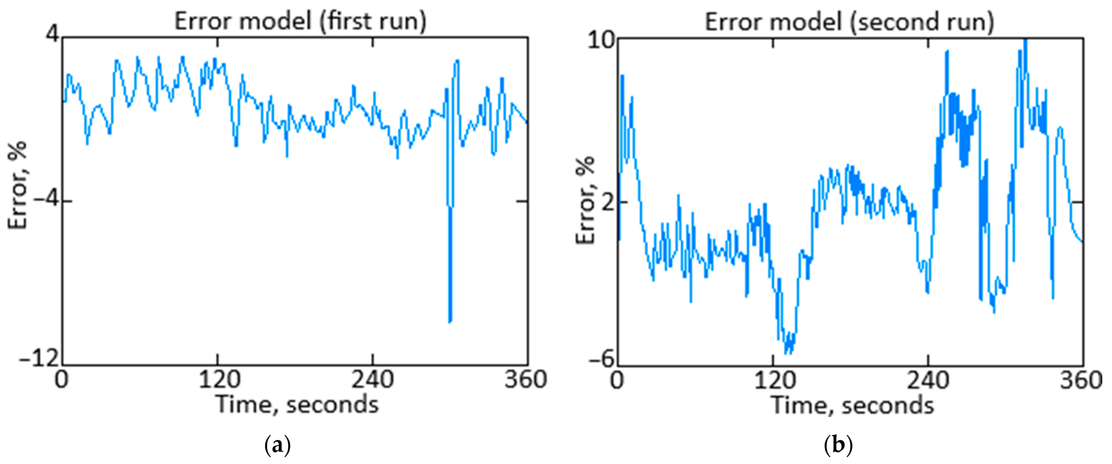
It is noted that the first engine start was carried out at an ambient temperature of 15 °C (288 K), and the second engine start was carried out at an ambient temperature of 24 °C (297 K). Figure 7 shows the model error value by time. The obtained model average error by simulation time at the first start was 1.035% (see Figure 7a), and at the second start was 2.576% (see Figure 7b).
At temperatures close to normal (288 K), the model demonstrated more accurate results compared to a temperature of 297 K. This discrepancy arises because the model was developed based on data obtained at 288 K. Additionally, adjusting parameters to standard conditions yields precise results only within a narrow range around normal conditions; greater deviations lead to increased computational errors. The adjusted parameters used in this case were justified as the tests were conducted with zero airflow velocity, at normal pressure, and within a small temperature range, resulting in minimal environmental impact on the simulation results. Model accuracy could be enhanced by conducting engine tests to generate additional curves for the gas-generator rotor acceleration. Further refinement may include expanding the temperature range and incorporating more detailed operational data.
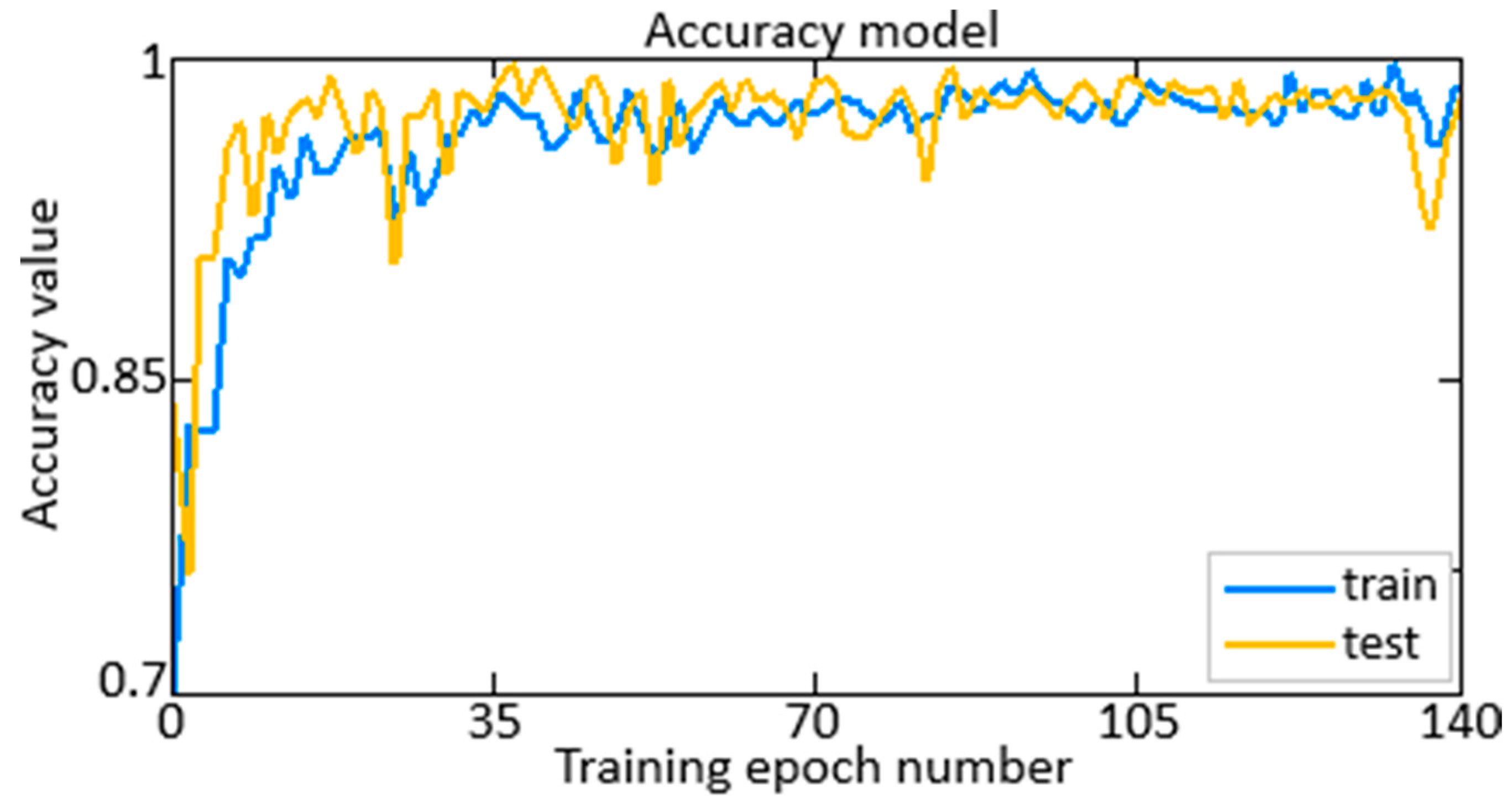
To validate the model, the following metrics were used: Accuracy, Precision, Recall, F1-measure, AUC-ROC [53,54,55,56,57]. The Accuracy metric is employed (see Figure 8) and is calculated at training epoch t using the following expression:
A c c u r a c y t = 1 N i = 1 N 1 y ^ i t = y t ,
where yi represents the i-th example true label, y ^ i t denotes the label predicted by the model for the i-th example, N signifies the examples total number in the dataset (whether training or validation), and 1 y ^ i t = y t is the indicator function that equals 1 if y ^ i t = y t and 0 otherwise.
The achieved accuracy of 99.3% in neural network modeling for sensor failure detection in helicopter TE systems indicates a high level of performance and reliability. This result reflects the model’s effectiveness in correctly identifying sensor failure and normal conditions, demonstrating its potential for accurate fault diagnosis and operational safety. The high accuracy underscores the robustness of the neural network in handling the complex patterns associated with sensor data.
Precision measures the correctly identified failure among all cases in proportion where the model predicted a failure. High precision means that the model rarely makes a mistake when predicting a failure. Recall measures the actual failure correctly detected by the model. High recall means that the model effectively finds most instances of real failure, although there may be false alarms. The F1-score is the precision and recall harmonic mean and provides a single metric for assessing both precision and recall. It is useful when it is important to account for both false alarms and missed instances of failure. Precision, Recall, and F1-measure are defined as:
P r e c i s i o n = T P T P + F P ,   R e c a l l = T P T P + F N ,   F 1 = 2 P r e c i s i o n R e c a l l P r e c i s i o n + R e c a l l ,
where TP (True Positives) is the correctly classified failure number, FP (False Positives) is the number of false alarms where the model incorrectly classified a normal condition as a failure, FN (False Negatives) is the instances of failure that were not detected by the model (Table 3) [58,59].
The metrics Precision = 0.987, Recall = 1.0, and F1-score = 0.993 in neural network modeling for sensor failure detection in helicopter TE systems indicate exceptional performance. A Precision = 0.987 signifies that the model maintains a high level of accuracy in predicting failure, while a Recall = 1.0 demonstrates complete sensitivity in identifying all actual instances of failure. The F1-score = 0.993 reflects a well-balanced performance, integrating both high precision and recall, which underscores the model’s robustness and reliability in fault detection.
A receiver operating characteristic (ROC) analysis is a crucial tool for evaluating the performance of a neural network model in detecting sensor failure in helicopter gas turbine engine systems. The ROC curve plots the true positive rate (TPR) against the false positive rate (FPR) at various threshold settings, providing a graphical representation of the model’s diagnostic ability across different decision thresholds. The TPR measures the proportion of actual failure correctly identified by the model. A high TPR indicates that the model effectively detects most instances of true failure. The FPR measures the proportion of normal conditions incorrectly classified as failure. A low FPR indicates that the model infrequently generates false alarms. TPR and FPR are defined as:
T P R = T P T P + F N ,   F P R = F P F P + T N .
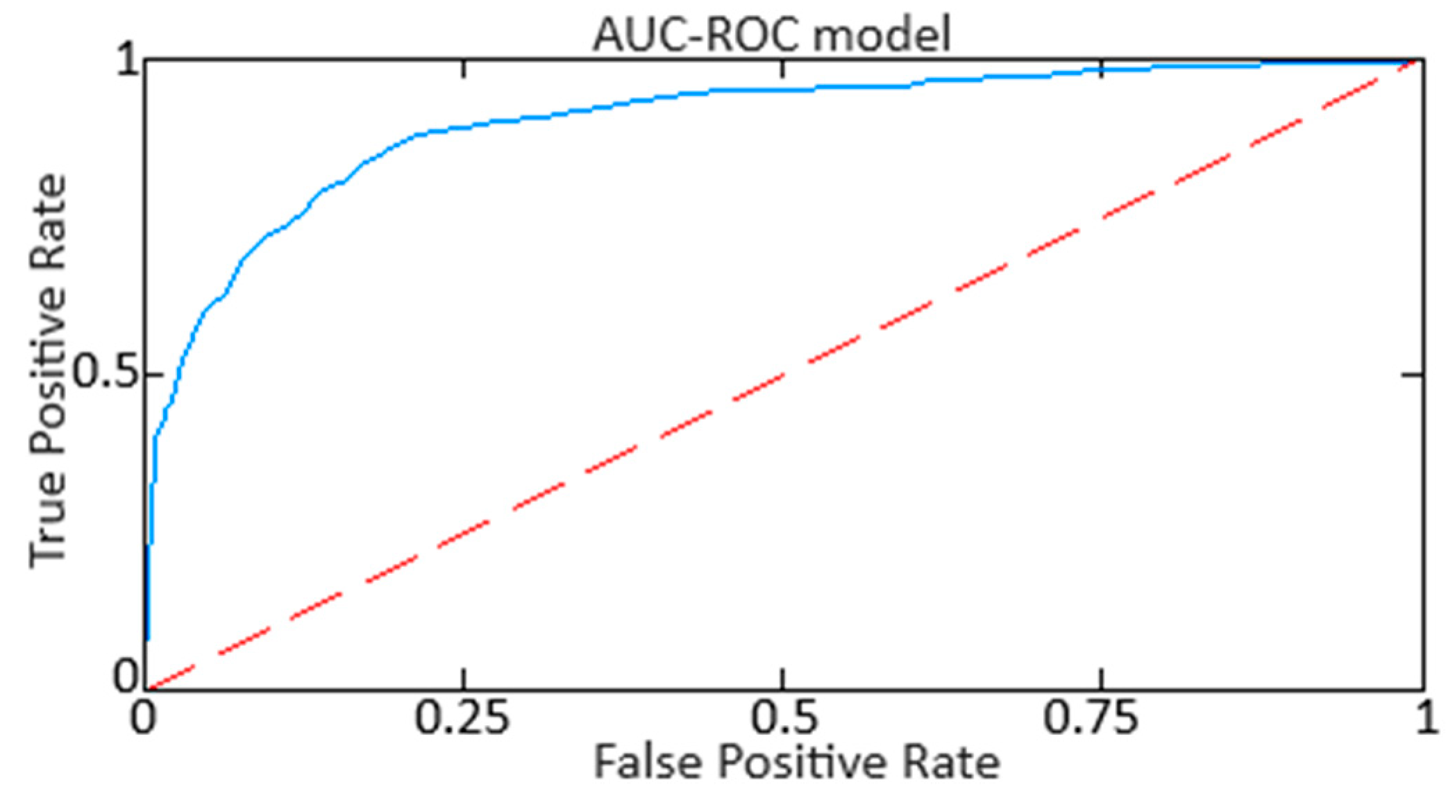
The AUC-ROC is a quantitative metric (see Figure 9) that signifies the likelihood that the model accurately identifies a randomly chosen positive instance as being more likely to be positive than a randomly chosen negative instance. The area under the ROC curve is expressed as:
A U C R O C = 0 1 T P R F P R 1 t d t ,
where TPR represents sensitivity, and FPR−1 is the false positive rate inverse (where 1 denotes specificity), with t denoting the classification threshold value ranging from 0 to 1.
The area under the ROC curve (AUC) of 0.874 in neural network modeling for sensor failure detection in helicopter TE systems indicates a strong performance in distinguishing between failure and normal conditions. An AUC = 0.874 suggests that the model demonstrates a correctly classifying high probability of a randomly selected failure as more likely to be a failure than a randomly selected normal condition. This value reflects the model’s effective discriminative ability and overall reliability in detecting sensor anomalies.

4. Discussion

The research focuses on advanced research in the helicopter TE neural network monitoring and control during flight operations. A method for the helicopter TE parameters neural network modeling during the gas-generator rotor r.p.m. failure (sensor disconnection) under various scenarios is proposed. A mathematical model (1)–(7) is developed to simulate TE failure in helicopters, encompassing both single and cascading failure. Model (1)–(7) employs differential equations to describe system dynamics, considering coefficient changes occurring during failure, such as compressor blade breakage or combustion chamber burnout. Additionally, model (1)–(7) incorporates time-varying coefficient changes and external disturbances, allowing for more accurate representation of both the immediate and long-term effects of failure.
The NARX neural network architecture choice is justified, and its training algorithm, based on the backpropagation algorithm, is developed. This NARX training algorithm application has achieved 99.3% accuracy (see Figure 8) in modeling the neural network for detecting failure (sensor disconnection) in the helicopter TE systems gas-generator rotor speed, demonstrating a high level of performance and reliability.
In research similar to the current study [60,61,62,63,64,65], three types of genetic algorithms were researched (Table 4). The first type explores the entire search space and is not directed, for which the best solutions may be lost and require significant search time. The second type is directional, for which it is possible to reach a local optimum. The third type is combined, that is, it combines the search focus with the entire search space research. To select the most effective training algorithm, numerical research was carried out, which results are presented in Table 5. To evaluate the effectiveness, criteria such as the number of iterations and identification accuracy number were chosen.
According to the comparison results (see Table 5), the genetic algorithm of all three types has the smallest number of iterations, however, the modeling for helicopter TE parameters neural network during the gas-generator rotor failure (sensor disconnection) solved by the task accuracy indicator when using the proposed algorithm is 4.19% higher than when using the genetic algorithm of type 3 (what is critical at helicopter flight mode), which gives the highest accuracy of all three types of genetic algorithms. A similar situation arises when comparing the loss indicator. Thus, the proposed algorithm in the neural network training task is most suitable for the network training procedure.
To validate a helicopter TE model based on a NARX neural network and mathematical model (1)–(7) for simulating helicopter engine failure, a hardware-in-the-loop simulation testbed (see Figure 4) was developed. This testbed operates within the Matlab Simulink graphical environment, featuring data exchange channels, a fuel metering valve simulator, a visualization and recording system, and other components (see Figure 5). For model verification, a sensor failure was simulated in the sensor simulator’s output electrical circuit; during the gas-generator rotor speed nTC control loop operation, an nTC sensor open circuit was simulated, detected by the built-in control system, and signaled as a “sensor break” (SB), followed by a “measuring channel failure” (MCF), which led to the neural network reconfiguration to regulate a pressure increase while fixing the sensor value at the last reliable level until the failure was resolved (see Figure 6). The first engine start at 15 °C (288 K) showed an average model error of 1.04% (see Figure 7a), and the second start at 24 °C (249 K) showed an error of 2.58% (see Figure 7), which is attributed to the model being created based on 288 K data, where deviations from normal conditions increase computational errors; however, in this case, parameter normalization was justified due to minimal environmental impact, and model accuracy can be improved through additional engine testing.
Computed metrics Precision = 0.987, Recall = 1.0, and F1-score = 0.993 demonstrate high accuracy, complete sensitivity, and balanced model performance, confirming its reliability in fault detection. Computed AUC = 0.874 (see Figure 9) shows strong model capability to distinguish between failure and normal conditions, confirming its effectiveness and reliability in anomaly detection.
The proposed helicopter TE neural network monitoring and control model, despite demonstrating high accuracy and reliability in fault detection as indicated by metrics such as Precision, Recall, F1-score, and AUC, is subject to several limitations. Firstly, the model’s accuracy is highly dependent on the environmental conditions used during its development, as evidenced by the increased error observed at temperatures deviating from the baseline of 288 K. This suggests that the model’s generalizability across varying operational environments may be limited. Additionally, the genetic algorithm comparison revealed that, while the proposed training algorithm outperforms in accuracy, it may require further optimization to reduce computational complexity and ensure robustness across a wider range of failure scenarios. Furthermore, the hardware-in-the-loop simulation, though effective for validation purposes, may not fully capture the intricacies of real-world operations, necessitating further testing and refinement in actual flight conditions.
Future research should focus on enhancing the model’s adaptability to diverse environmental conditions [68,69,70,71] and further optimizing the training algorithms to reduce computational complexity [72,73,74,75]. Additionally, validating the model in real-world flight scenarios will be crucial to ensure its robustness and applicability in operational environments.

5. Conclusions

The research presents a sophisticated approach to monitoring and controlling helicopter turboshaft engines during flight operations by employing neural network models to address gas-generator rotor failure, such as sensor disconnections. A detailed mathematical model was developed to simulate various failure scenarios, including both single and cascading failure. This model uses differential equations to represent system dynamics and incorporates time-varying coefficients and external disturbances, allowing for a nuanced depiction of failure effects like compressor blade breakage or combustion chamber burnout.
The NARX neural network architecture and its associated training algorithm choice, based on backpropagation, has demonstrated a high level of accuracy, achieving 99.3% in detecting sensor disconnections. This performance highlights the effectiveness of the NARX model in accurately modeling the gas-generator rotor r.p.m., contributing significantly to the reliability of fault detection systems in helicopter turboshaft engines.
In comparing different genetic algorithms for training the neural network, three types were analyzed: non-directional, directional, and combined. Numerical research revealed that the proposed algorithm surpasses the combined genetic algorithm type in accuracy by 4.19%, despite both having a similar iteration count. This indicates that the proposed training algorithm is more effective for the task, offering enhanced precision and reduced computational complexity compared to other methods.
A hardware-in-the-loop simulation testbed was developed to validate the NARX model and mathematical framework. The testbed, operating within the Matlab Simulink environment, successfully simulated sensor failure and demonstrated high model accuracy with an average error of 1.04% at 15 °C and 2.58% at 24 °C. Metrics such as Precision (0.987), Recall (1.0), F1-score (0.993), and AUC (0.874) confirm the model’s effectiveness in detecting failure and distinguishing between fault and normal conditions. However, limitations include sensitivity to environmental conditions and the need for further optimization and real-world validation to ensure robustness across various operational scenarios. Future research should focus on enhancing the model’s adaptability and optimizing the training algorithms to address these challenges.

Author Contributions

Conceptualization, S.V.; methodology, S.V. and V.V.; software, V.V.; validation, A.S. and V.V.; formal analysis, S.V.; investigation, A.S.; resources, V.S. and O.M.; data curation, A.S. and V.V.; writing—original draft preparation, S.V.; writing—review and editing, A.S.; visualization, V.V.; supervision, V.S. and O.M.; project administration, V.S. and O.M.; funding acquisition, A.S. All authors have read and agreed to the published version of the manuscript.

Funding

This research received no external funding.

Data Availability Statement

Data is contained within the article.

Acknowledgments

In this section, you can acknowledge any support given which is not covered by the author contribution or funding sections. This may include administrative and technical support, or donations in kind (e.g., materials used for experiments).

Conflicts of Interest

The authors declare no conflicts of interest.

References

  1. Lan, J.; Patton, R.J.; Punta, E. Fault-Tolerant Tracking Control for A 3-DOF Helicopter with Actuator Faults and Saturation. IFAC-PapersOnLine 2017, 50, 5250–5255. [Google Scholar] [CrossRef]
  2. Pérez-Ventura, U.; Fridman, L.; Capello, E.; Punta, E. Fault Tolerant Control Based on Continuous Twisting Algorithms of a 3-DoF Helicopter Prototype. Control Eng. Pract. 2020, 101, 104486. [Google Scholar] [CrossRef]
  3. Ma, Y.; Zhang, K.; Jiang, B. Practical Prescribed-Time Active Fault-Tolerant Control for Mixed-Order Heterogeneous Multiagent Systems: A Fully Actuated System Approach. Automatica 2024, 166, 111721. [Google Scholar] [CrossRef]
  4. Vladov, S.; Yakovliev, R.; Vysotska, V.; Nazarkevych, M.; Lytvyn, V. The Method of Restoring Lost Information from Sensors Based on Auto-Associative Neural Networks. Appl. Syst. Innov. 2024, 7, 53. [Google Scholar] [CrossRef]
  5. Zhu, X.; Li, D. Robust Fault Estimation for a 3-DOF Helicopter Considering Actuator Saturation. Mech. Syst. Signal Process. 2021, 155, 107624. [Google Scholar] [CrossRef]
  6. Kumar, S.R.; Devakumar, J. Recurrent Neural Network Based Sensor Fault Detection and Isolation for Nonlinear Systems: Application in PWR. Prog. Nucl. Energy 2023, 163, 104836. [Google Scholar] [CrossRef]
  7. Cheng, K.; Wang, Y.; Yang, X.; Zhang, K.; Liu, F. An Intelligent Online Fault Diagnosis System for Gas Turbine Sensors Based on Unsupervised Learning Method LOF and KELM. Sens. Actuators A Phys. 2024, 365, 114872. [Google Scholar] [CrossRef]
  8. Shen, Y.; Khorasani, K. Hybrid Multi-Mode Machine Learning-Based Fault Diagnosis Strategies with Application to Aircraft Gas Turbine Engines. Neural Netw. 2020, 130, 126–142. [Google Scholar] [CrossRef]
  9. Shuai, M.; Yafeng, W.; Hua, Z.; Linfeng, G. Parameter Modelling of Fleet Gas Turbine Engines Using Gated Recurrent Neural Networks. J. Phys. Conf. Ser. 2023, 2472, 012012. [Google Scholar] [CrossRef]
  10. Khattak, W.R.; Salman, A.; Ghafoor, S.; Latif, S. Multi-Modal LSTM Network for Anomaly Prediction in Piston Engine Aircraft. Heliyon 2024, 2024 10, e25120. [Google Scholar] [CrossRef]
  11. Boujamza, A.; Lissane Elhaq, S. Attention-Based LSTM for Remaining Useful Life Estimation of Aircraft Engines. IFAC-PapersOnLine 2022, 55, 450–455. [Google Scholar] [CrossRef]
  12. Bovsunovsky, A.; Nosal, O. Highly Sensitive Methods for Vibration Diagnostics of Fatigue Damage in Structural Elements of Aircraft Gas Turbine Engines. Procedia Struct. Integr. 2022, 35, 74–81. [Google Scholar] [CrossRef]
  13. Wei, X.; Yingqing, G. Aircraft Engine Sensor Fault Diagnostics Based on Estimation of Engine’s Health Degradation. Chin. J. Aeronaut. 2009, 22, 18–21. [Google Scholar] [CrossRef]
  14. Szrama, S.; Lodygowski, T. Aircraft Engine Remaining Useful Life Prediction Using Neural Networks and Real-Life Engine Operational Data. Adv. Eng. Softw. 2024, 192, 103645. [Google Scholar] [CrossRef]
  15. Zhao, J.; Li, Y.-G.; Sampath, S. A Hierarchical Structure Built on Physical and Data-Based Information for Intelligent Aero-Engine Gas Path Diagnostics. Appl. Energy 2023, 332, 120520. [Google Scholar] [CrossRef]
  16. Weiser, C.; Ossmann, D. Fault-Tolerant Control for a High Altitude Long Endurance Aircraft. IFAC-PapersOnLine 2022, 55, 724–729. [Google Scholar] [CrossRef]
  17. Jiang, W.; Xu, Y.; Chen, Z.; Zhang, N.; Xue, X.; Zhou, J. Measurement of Health Evolution Tendency for Aircraft Engine Using a Data-Driven Method Based on Multi-Scale Series Reconstruction and Adaptive Hybrid Model. Measurement 2022, 199, 111502. [Google Scholar] [CrossRef]
  18. Li, B.; Zhao, Y.-P.; Chen, Y.-B. Unilateral Alignment Transfer Neural Network for Fault Diagnosis of Aircraft Engine. Aerosp. Sci. Technol. 2021, 118, 107031. [Google Scholar] [CrossRef]
  19. Skarka, W.; Nalepa, R.; Musik, R. Integrated Aircraft Design System Based on Generative Modelling. Aerospace 2023, 10, 677. [Google Scholar] [CrossRef]
  20. Baláž, M.; Kováčiková, K.; Novák, A.; Vaculík, J. The Application of Internet of Things in Air Transport. Transp. Res. Procedia 2023, 75, 60–67. [Google Scholar] [CrossRef]
  21. Bouzidi, Z.; Terrissa, L.S.; Zerhouni, N.; Ayad, S. An Efficient Cloud Prognostic Approach for Aircraft Engines Fleet Trending. Int. J. Comput. Appl. 2018, 42, 514–529. [Google Scholar] [CrossRef]
  22. Vladov, S.; Yakovliev, R.; Hubachov, O.; Rud, J.; Stushchanskyi, Y. Neural Network Modeling of Helicopters Turboshaft Engines at Flight Modes Using an Approach Based on “Black Box” Models. CEUR Workshop Proc. 2024, 3624, 116–135. [Google Scholar]
  23. Vysotska, V.; Vladov, S.; Yakovliev, R.; Yurko, A. Hybrid Neural Network Identifying Complex Dynamic Objects: Comprehensive Modelling and Training Method Modification. CEUR Workshop Proc. 2024, 3702, 124–143. [Google Scholar]
  24. Vladov, S.; Shmelov, Y.; Yakovliev, R. Modified Searchless Method for Identification of Helicopters Turboshaft Engines at Flight Modes Using Neural Networks. In Proceedings of the 2022 IEEE 3rd KhPI Week on Advanced Technology (KhPIWeek), Kharkiv, Ukraine, 3–7 October 2022; pp. 257–262. [Google Scholar] [CrossRef]
  25. Wei, Z.; Zhang, S.; Jafari, S.; Nikolaidis, T. Gas Turbine Aero-Engines Real Time on-Board Modelling: A Review, Research Challenges, and Exploring the Future. Prog. Aerosp. Sci. 2020, 121, 100693. [Google Scholar] [CrossRef]
  26. Yang, Q.; Tang, B.; Li, Q.; Liu, X.; Bao, L. Dual-Frequency Enhanced Attention Network for Aircraft Engine Remaining Useful Life Prediction. ISA Trans. 2023, 141, 167–183. [Google Scholar] [CrossRef]
  27. Zaidan, M.A.; Harrison, R.F.; Mills, A.R.; Fleming, P.J. Bayesian Hierarchical Models for Aerospace Gas Turbine Engine Prognostics. Expert Syst. Appl. 2015, 42, 539–553. [Google Scholar] [CrossRef]
  28. Kumar, R.; Kumar, V.S.; Butt, M.M.; Sheikh, N.A.; Khan, S.A.; Afzal, A. Thermo-Mechanical Analysis and Estimation of Turbine Blade Tip Clearance of a Small Gas Turbine Engine under Transient Operating Conditions. Appl. Therm. Eng. 2020, 179, 115700. [Google Scholar] [CrossRef]
  29. Zhou, D.; Huang, D.; Zhang, H.; Yang, J. Periodic Analysis on Gas Path Fault Diagnosis of Gas Turbines. ISA Trans. 2022, 129, 429–441. [Google Scholar] [CrossRef]
  30. Zhu, P.; Yu, L.; Zeng, J. Prescribed Performance Control for Nonlinear Parameter-Varying Systems with an Application to Turbofan Engine. J. Frankl. Inst. 2023, 360, 7722–7738. [Google Scholar] [CrossRef]
  31. Vladov, S.; Kovtun, V.; Sokurenko, V.; Muzychuk, O.; Vysotska, V. The Helicopter Turboshaft Engine’s Reconfigured Dynamic Model for Functional Safety Estimation. Electronics 2024, 13, 3477. [Google Scholar] [CrossRef]
  32. Ibrahem, I.M.A.; Akhrif, O.; Moustapha, H.; Staniszewski, M. Nonlinear Generalized Predictive Controller Based on Ensemble of NARX Models for Industrial Gas Turbine Engine. Energy 2021, 230, 120700. [Google Scholar] [CrossRef]
  33. Amirkhani, S.; Tootchi, A.; Chaibakhsh, A. Fault Detection and Isolation of Gas Turbine Using Series–Parallel NARX Model. ISA Trans. 2022, 120, 205–221. [Google Scholar] [CrossRef] [PubMed]
  34. Feng, H.; Liu, B.; Xu, M.; Li, M.; Song, Z. Model-Based Deduction Learning Control: A Novel Method for Optimizing Gas Turbine Engine Afterburner Transient. Energy 2024, 292, 130512. [Google Scholar] [CrossRef]
  35. Fedorov, E.; Dikova, Y. Development of the method of prediction of content of explosive gases in mines. Sci. Pap. Donetsk Natl. Tech. Univ. Ser. Inform. Cybern. Comput. Sci. 2015, 1, 97–104. [Google Scholar]
  36. Vladov, S.; Yakovliev, R.; Bulakh, M.; Vysotska, V. Neural Network Approximation of Helicopter Turboshaft Engine Parameters for Improved Efficiency. Energies 2024, 17, 2233. [Google Scholar] [CrossRef]
  37. Vladov, S.; Scislo, L.; Sokurenko, V.; Muzychuk, O.; Vysotska, V.; Osadchy, S.; Sachenko, A. Neural Network Signal Integration from Thermogas-Dynamic Parameter Sensors for Helicopters Turboshaft Engines at Flight Operation Conditions. Sensors 2024, 24, 4246. [Google Scholar] [CrossRef]
  38. Vladov, S.; Shmelov, Y.; Yakovliev, R.; Petchenko, M. Neural Network Method for Parametric Adaptation Helicopters Turboshaft Engines On-Board Automatic Control System Parameters. CEUR Workshop Proc. 2023, 3403, 179–195. [Google Scholar]
  39. Kim, H.-Y. Statistical Notes for Clinical Researchers: Chi-Squared Test and Fisher’s Exact Test. Restor. Dent. Endod. 2017, 42, 152. [Google Scholar] [CrossRef]
  40. Stefanovic, C.M.; Armada, A.G.; Costa-Perez, X. Second Order Statistics of -Fisher-Snedecor Distribution and Their Application to Burst Error Rate Analysis of Multi-Hop Communications. IEEE Open J. Commun. Soc. 2022, 3, 2407–2424. [Google Scholar] [CrossRef]
  41. Babichev, S.; Krejci, J.; Bicanek, J.; Lytvynenko, V. Gene expression sequences clustering based on the internal and external clustering quality criteria. In Proceedings of the 2017 12th International Scientific and Technical Conference on Computer Sciences and Information Technologies (CSIT), Lviv, Ukraine, 5–8 September 2017. [Google Scholar] [CrossRef]
  42. Hu, Z.; Kashyap, E.; Tyshchenko, O.K. GEOCLUS: A Fuzzy-Based Learning Algorithm for Clustering Expression Datasets. Lect. Notes Data Eng. Commun. Technol. 2022, 134, 337–349. [Google Scholar] [CrossRef]
  43. Kuznetsov, A.V.; Makaryants, G.M. Micro Gas Turbine Engine Imitation Model. Aerosp. Mech. Eng. 2017, 16, 65–74. [Google Scholar] [CrossRef]
  44. Denisova, E.V.; Chernikova, M.A. Development of semi-naturalistic modeling stands for studying the gas turbine engines automatic control systems. Mod. High Technol. 2019, 7, 122–131. [Google Scholar]
  45. Vladov, S.; Shmelov, Y.; Yakovliev, R. Optimization of Helicopters Aircraft Engine Working Process Using Neural Networks Technologies. CEUR Workshop Proc. 2022, 3171, 1639–1656. [Google Scholar]
  46. Kilic, U.; Yalin, G.; Cam, O. Digital Twin for Electronic Centralized Aircraft Monitoring by Machine Learning Algorithms. Energy 2023, 283, 129118. [Google Scholar] [CrossRef]
  47. Barthorpe, R.J.; Worden, K. Emerging Trends in Optimal Structural Health Monitoring System Design: From Sensor Placement to System Evaluation. J. Sens. Actuator Netw. 2020, 9, 31. [Google Scholar] [CrossRef]
  48. Shubyn, B.; Maksymyuk, T.; Gazda, J.; Rusyn, B.; Mrozek, D. Federated Learning: A Solution for Improving Anomaly Detection Accuracy of Autonomous Guided Vehicles in Smart Manufacturing. Lect. Notes Electr. Eng. 2024, 1198, 746–761. [Google Scholar] [CrossRef]
  49. Rusyn, B.; Lutsyk, O.; Kosarevych, R.; Obukh, Y. Application Peculiarities of Deep Learning Methods in the Problem of Big Datasets Classification. Lect. Notes Electr. Eng. 2021, 831, 493–506. [Google Scholar] [CrossRef]
  50. Li, S.; Wang, Y.; Zhang, H. Research on Adaptive Feedforward Control Method for Tiltrotor Aircraft/Turboshaft Engine System Based on Radial Basis Function Neural Network. Aerosp. Sci. Technol. 2024, 150, 109180. [Google Scholar] [CrossRef]
  51. Wang, Y.-Q.; Zhao, Y.-P. A Novel Inter-Domain Attention-Based Adversarial Network for Aero-Engine Partial Unsupervised Cross-Domain Fault Diagnosis. Eng. Appl. Artif. Intell. 2023, 123, 106486. [Google Scholar] [CrossRef]
  52. Wang, Y.; Ji, C.; Xi, Z.; Zhang, H.; Zhao, Q. An Adaptive Matching Control Method of Multiple Turboshaft Engines. Eng. Appl. Artif. Intell. 2023, 123, 106496. [Google Scholar] [CrossRef]
  53. Pasieka, M.; Grzesik, N.; Kuźma, K. Simulation modeling of fuzzy logic controller for aircraft engines. Int. J. Comput. 2017, 16, 27–33. [Google Scholar] [CrossRef]
  54. Andriushchenko, K.; Rudyk, V.; Riabchenko, O.; Kachynska, M.; Marynenko, N.; Shergina, L.; Kovtun, V.; Tepliuk, M.; Zhemba, A.; Kuchai, O. Processes of managing information infrastructure of a digital enterprise in the framework of the «Industry 4.0» concept. East. Eur. J. Enterp. Technol. 2019, 1, 60–72. [Google Scholar] [CrossRef]
  55. Cherrat, E.M.; Alaoui, R.; Bouzahir, H. Score fusion of finger vein and face for human recognition based on convolutional neural network model. Int. J. Comput. 2020, 19, 11–19. [Google Scholar] [CrossRef]
  56. Hu, Z.; Dychka, I.; Potapova, K.; Meliukh, V. Augmenting Sentiment Analysis Prediction in Binary Text Classification through Advanced Natural Language Processing Models and Classifiers. Int. J. Inf. Technol. Comput. Sci. 2024, 16, 16–31. [Google Scholar] [CrossRef]
  57. Vladov, S.; Yakovliev, R.; Hubachov, O.; Rud, J. Neuro-Fuzzy System for Detection Fuel Consumption of Helicopters Turboshaft Engines. CEUR Workshop Proc. 2023, 3628, 628–647. [Google Scholar]
  58. Kovtun, V.; Altameem, T.; Al-Maitah, M.; Kempa, W. Entropy-Metric Estimation of the Small Data Models with Stochastic Parameters. Heliyon 2024, 10, e24708. [Google Scholar] [CrossRef]
  59. Kovtun, V.; Grochla, K.; Połys, K. Investigation of the Information Interaction of the Sensor Network End IoT Device and the Hub at the Transport Protocol Level. Electronics 2023, 12, 4662. [Google Scholar] [CrossRef]
  60. Xu, Z.; Pei, J.; Ding, S.; Chen, L.; Zhao, S.; Shen, X.; Zhu, K.; Shao, L.; Zhong, Z.; Yan, H.; et al. Gas Exchange Optimization in Aircraft Engines Using Sustainable Aviation Fuel: A Design of Experiment and Genetic Algorithm Approach. Energy AI 2024, 17, 100396. [Google Scholar] [CrossRef]
  61. Feng, X.; Zhu, X.; Zhao, W.; Yan, C. Coupling Mechanical Model and Failure of Aeroengine Ceramic Matrix Composite Based on Genetic Algorithm. Meas. Sens. 2024, 33, 101226. [Google Scholar] [CrossRef]
  62. Aygun, H.; Turan, O. Application of Genetic Algorithm in Exergy and Sustainability: A Case of Aero-Gas Turbine Engine at Cruise Phase. Energy 2022, 238, 121644. [Google Scholar] [CrossRef]
  63. Jafari, S.; Nikolaidis, T. Meta-Heuristic Global Optimization Algorithms for Aircraft Engines Modelling and Controller Design; A Review, Research Challenges, and Exploring the Future. Prog. Aerosp. Sci. 2019, 104, 40–53. [Google Scholar] [CrossRef]
  64. Khan, N.; Abdi, S.A.A.; Khan, T.A.; Rizvi, S.S.A. Minimization of High Maintenance Cost and Hazard Emissions Related to Aviation Engines: An Implementation of Functions Optimizations by Using Genetic Algorithm for Better Performance. Eng. Proc. 2023, 46, 11. [Google Scholar] [CrossRef]
  65. Iuspa, L.; Scaramuzzino, F.; Petrenga, P. Optimal Design of an Aircraft Engine Mount via Bit-Masking Oriented Genetic Algorithms. Adv. Eng. Softw. 2003, 34, 707–720. [Google Scholar] [CrossRef]
  66. Rusyn, B.; Lutsyk, O.; Kosarevych, R.; Kapshii, O.; Karpin, O.; Maksymyuk, T.; Gazda, J. Rethinking Deep CNN Training: A Novel Approach for Quality-Aware Dataset Optimization. IEEE Access 2024, 12, 137427–137438. [Google Scholar] [CrossRef]
  67. Vladov, S.; Shmelov, Y.; Yakovliev, R.; Petchenko, M.; Drozdova, S. Neural Network Method for Helicopters Turboshaft Engines Working Process Parameters Identification at Flight Modes. In Proceedings of the 2022 IEEE 4th International Conference on Modern Electrical and Energy System (MEES), Kremenchuk, Ukraine, 20–22 October 2022. [Google Scholar] [CrossRef]
  68. Vlasenko, D.; Inkarbaieva, O.; Peretiatko, M.; Kovalchuk, D.; Sereda, O. Helicopter Radio System for Low Altitudes and Flight Speed Measuring with Pulsed Ultra-Wideband Stochastic Sounding Signals and Artificial Intelligence Elements. Radioelectron. Comput. Syst. 2023, 3, 48–59. [Google Scholar] [CrossRef]
  69. de Voogt, A.; Nero, K. Technical Failures in Helicopters: Non-Powerplant-Related Accidents. Safety 2023, 9, 10. [Google Scholar] [CrossRef]
  70. de Voogt, A.; St. Amour, E. Safety of Twin-Engine Helicopters: Risks and Operational Specificity. Saf. Sci. 2021, 136, 105169. [Google Scholar] [CrossRef]
  71. Wei, Y.; Chen, R.; Yuan, Y.; Wang, L. Influence of Engine Dynamic Characteristics on Helicopter Handling Quality in Hover and Low-Speed Forward Flight. Aerospace 2023, 11, 34. [Google Scholar] [CrossRef]
  72. Bisikalo, O.; Danylchuk, O.; Kovtun, V.; Kovtun, O.; Nikitenko, O.; Vysotska, V. Modeling of Operation of Information System for Critical Use in the Conditions of Influence of a Complex Certain Negative Factor. Int. J. Control Autom. Syst. 2022, 20, 1904–1913. [Google Scholar] [CrossRef]
  73. Turchenko, V.; Chalmers, E.; Luczak, A. A deep convolutional auto-encoder with pooling–Unpooling layers in caffe. Int. J. Comput. 2019, 1, 8–31. [Google Scholar] [CrossRef]
  74. Altameem, A.; Al-Ma’aitah, M.; Kovtun, V.; Altameem, T. A Computationally Efficient Method for Assessing the Impact of an Active Viral Cyber Threat on a High-Availability Cluster. Egypt. Inform. J. 2023, 24, 61–69. [Google Scholar] [CrossRef]
  75. Xia, H. Modeling and Control Strategy of Small Unmanned Helicopter Rotation Based on Deep Learning. Syst. Soft Comput. 2024, 6, 200146. [Google Scholar] [CrossRef]
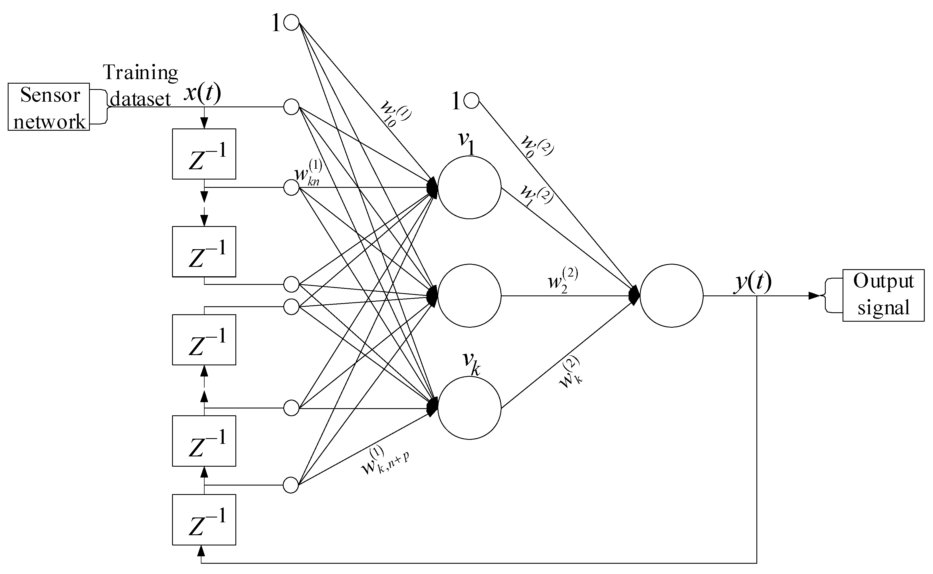
Figure 1. The proposed nonlinear autoregression neural network with exogenous inputs (NARX).
Jsan 13 00066 g001
Figure 2. The TV3-117 turboshaft engine parameters dynamics time series using digitized oscillograms: (black curve): Gas-generator rotor r.p.m; (green curve) Free turbine rotor speed; (red curve) Gas temperature in front of the compressor turbine (author’s research).
Jsan 13 00066 g002
Figure 3. Cluster analysis results: (a) Training dataset, (b) Test dataset (author’s research).
Jsan 13 00066 g003
Figure 4. Scheme of the helicopter turboshaft engine model with the semi-physical modeling stand interaction (author’s research).
Jsan 13 00066 g004
Figure 5. Overall view of the NARX neural network interaction with the semi-physical modeling stand implementation within the Matlab Simulink environment (author’s research).
Jsan 13 00066 g005
Figure 6. Resulting diagrams: (ac) are the simulated engine thermogas-dynamic parameters taking into account sensor break; (df) are the discrete signals during the engine model reconfiguration (author’s research).
Jsan 13 00066 g006aJsan 13 00066 g006b
Figure 7. Diagram of the model error magnitude over time: (a) On the first run, (b) On the second run (author’s research).
Jsan 13 00066 g007
Figure 8. Accuracy metric diagram (author’s research).
Jsan 13 00066 g008
Figure 9. The obtained AUC-ROC curve (author’s research).
Jsan 13 00066 g009
Table 1. Failure and corresponding time-varying changes in system matrices [31].
Failure Type\Impact AspectMeasurement AccuracySystem ReliabilityOperation under Extreme ConditionsResponse TimeEconomic ImpactSafety
Instantaneous failureHighReducedNot relevantImmediate disruptionHigh costsHigh risk
Intermittent failureMediumUnstableMay be hinderedDelaysPotential additional costsMedium risk
Partial failureAccuracy degradationPartialDepends on the situationPossible delaysAdditional costs for correctionMedium risk
Multiple failureVery high errorCriticalCriticalSignificant delaysSignificant economic lossesCritical risk
Drift failureGradual degradationGradual degradationMay be problematicDelaysGradual additional costsMedium risk
Systematic failureConstant degradationConstant degradationMay be hinderedStable slowdownHigh economic lossesMedium risk
Random failureUnpredictable impactUnpredictable impactMay be problematicUncertainUnpredictable costsMedium risk
Material degradation failureGradual degradationGradual degradationMay be problematicDelaysGradual additional costsMedium risk
Thermal failureAccuracy degradationTemporary or permanentCriticalSlowdownHigh replacement costsHigh risk
Vibration failureUnpredictable impactUnpredictableCriticalPossible delaysPotential additional costsHigh risk
Moisture failureGradual degradationGradual degradationCriticalSlowdownHigh repair costsMedium risk
Electromagnetic interference failureAccuracy degradationPossible issuesMay be hinderedPossible delaysAdditional shielding costsMedium risk
Software failureUnpredictable impactUnpredictableMay be problematicSlowdownHigh software correction costsMedium risk
Leakage current failureAccuracy degradationTemporary or permanentNot relevantSlowdownHigh replacement costsHigh risk
Table 2. The training dataset fragment (author’s research).
Value14396160211235256
nTC0.6860.9720.9030.9040.9120.7410.824
nFT0.5320.9870.7460.7530.7620.4550.506
T G * 0.4880.9800.7120.7220.7240.5190.522
Table 3. The error matrix (author’s research).
Actual\PredictedFailureNormalDescription
FailureTPFNTP (True Positives) is the cases number where the model correctly predicted a failure
FP (False Positives) is the cases number where the model incorrectly predicted a failure, although no failure was present
TN (True Negatives) is the cases number where the model correctly predicted no failure
FN (False Negatives) is the cases number where the model failed to detect a real failure
NormalFPTN
Table 4. Three types of genetic algorithm structures used in this research [60,62].
Genetic Algorithm OperatorsGenetic Algorithm Types
Type 1Type 2Type 3
ReproductionEquiprobable selectionLinearly ordered selectionThe equiprobable and linearly combination ordered selection
Crossing overEqually probable, individuals’ selection is the best individuals with the worst crossingEqually probable, individuals’ selection is the best individuals with the best crossingEqually probable, selection of individuals is the crossing the best individuals with the worst and the best individuals with the best combination
MutationHomogeneous with high probabilityHomogeneous with low probabilityHeterogeneous
ReductionEquiprobable schemeSelection schemeThe equiprobability and selection scheme combination
Table 5. Comparative analysis results [61,63,65,66,67].
Characteristic/AlgorithmProposed AlgorithmGenetic Algorithms
Type 1Type 2Type 3
Iterations 140130120120
Accuracy0.99380.92580.93360.9522
Loss0.00620.07420.06640.0478
Disclaimer/Publisher’s Note: The statements, opinions and data contained in all publications are solely those of the individual author(s) and contributor(s) and not of MDPI and/or the editor(s). MDPI and/or the editor(s) disclaim responsibility for any injury to people or property resulting from any ideas, methods, instructions or products referred to in the content.