A Nature-Inspired Partial Distance-Based Clustering Algorithm

Abstract

In the rapidly advancing landscape of digital technologies, clustering plays a critical role in the domains of artificial intelligence and big data. Clustering is essential for extracting meaningful insights and patterns from large, intricate datasets. Despite the efficacy of traditional clustering techniques in handling diverse data types and sizes, they encounter challenges posed by the increasing volume and dimensionality of data, as well as the complex structures inherent in high-dimensional spaces. This research recognizes the constraints of conventional clustering methods, including sensitivity to initial centroids, dependence on prior knowledge of cluster counts, and scalability issues, particularly in large datasets and Internet of Things implementations. In response to these challenges, we propose a K-level clustering algorithm inspired by the collective behavior of fish locomotion. K-level introduces a novel clustering approach based on greedy merging driven by distances in stages. This iterative process efficiently establishes hierarchical structures without the need for exhaustive computations. K-level gives users enhanced control over computational complexity, enabling them to specify the number of clusters merged simultaneously. This flexibility ensures accurate and efficient hierarchical clustering across diverse data types, offering a scalable solution for processing extensive datasets within a reasonable timeframe. The internal validation metrics, including the Silhouette Score, Davies–Bouldin Index, and Calinski–Harabasz Index, are utilized to evaluate the K-level algorithm across various types of datasets. Additionally, comparisons are made with rivals in the literature, including UPGMA, CLINK, UPGMC, SLINK, and K-means. The experiments and analyses show that the proposed algorithm overcomes many of the limitations of existing clustering methods, presenting scalable and adaptable clustering in the dynamic landscape of evolving data challenges.

1. Introduction

Today’s data-driven world poses challenges, such as data mining and knowledge discovery, for extracting meaningful insights from large and complex datasets. Clustering is a fundamental task in machine learning and data analysis for organizing and understanding datasets by grouping similar data points [1]. Clustering algorithms make it possible to uncover hidden patterns, discovering structure, and facilitating decision-making. Traditional clustering techniques encompass two main types: hierarchical techniques and partitional techniques. Within hierarchical techniques, popular methods include single linkage [2], average linkage [3], and complete linkage [4]. On the other hand, partitional techniques feature well-known approaches such as K-means [5,6], PAM [7], and CLARA [7]. Figure 1 depicts the traditional clustering techniques.

While these traditional clustering techniques have significantly progressed in handling various data types and sizes, capturing complex structures in high-dimensional spaces is challenged by the constant surge in data volume and dimensionality [8]. They are often sensitive to the choice of initial centroids or linkage criteria and necessitate prior knowledge of the number of clusters. Additionally, common clustering algorithms may struggle to maintain computational efficiency as datasets scale up. For instance, the time complexity of K-means can grow linearly with the number of data points, rendering it impractical for large datasets or implementation in Internet of Things (IoT) scenarios. While hierarchical clustering provides a more comprehensive view of data relationships, its quadratic time complexity can make it computationally infeasible for very large datasets [9]. Consequently, there is a pressing need for scalable clustering techniques capable of processing vast amounts of data within a reasonable time frame.

In this article, we propose a new clustering algorithm named K-level that addresses several of these limitations. The core idea of this approach is inspired by the collective behavior of fish locomotion, where a K-level algorithm innovatively merges clusters iteratively based on distances, creating hierarchical structures efficiently without exhaustive iterations. The algorithm offers enhanced control over computational complexity by specifying the number of clusters merged simultaneously, showcasing flexibility across diverse data types for accurate and efficient hierarchical clustering.

The rest of this article is structured as follows: The related work is presented in Section 2. Section 3 presents the proposed K-level partial distance-based clustering algorithm. Section 4 presents experiments and analyses to validate the proposed algorithm. Section 5 concludes the article and gives future work directions.

2. Related Work

Clustering remains a persistent research challenge as the development of robust algorithms continues to evolve. This section reviews existing clustering techniques through three major categories: hierarchical partitional and hybrid clustering. It investigates the unique characteristics of each category for a comprehensive analysis. Furthermore, we emphasize clustering’s significance in data-intensive processing environments by reviewing significant applications, aiming to demonstrate its practical value and relevance.

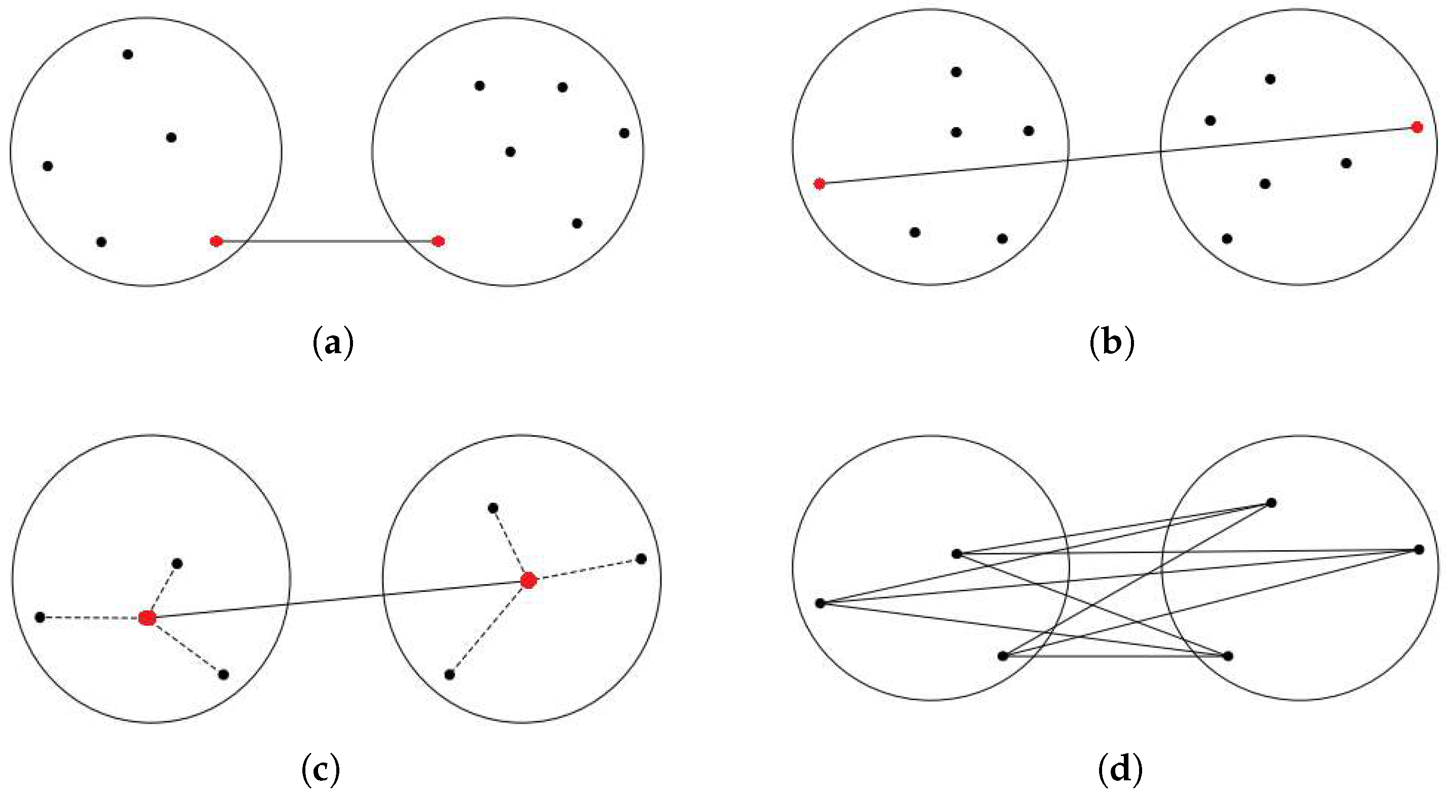
In the context of hierarchical algorithms, a dendrogram is generated to visually depict the hierarchical organization of patterns and their corresponding similarities within a dataset [10]. For instance, the single linkage (SLINK) [2] algorithm groups clusters in a bottom-up approach, as depicted in Figure 2a. At each step, SLINK merges two clusters that contain the nearest pair of objects not belonging to the same cluster. While useful in certain cases, the algorithm’s complexity is a drawback due to its sensitivity to outliers and noise. However, Figure 2b shows another type of agglomerative clustering, named complete linkage (CLINK) algorithm [4], which clusters data objects based on their pairwise maximum distances. The distance between two clusters is defined in this method as the greatest distance between any pair of data objects, one from each cluster. However, in most cases, relying solely on the nearest or farthest pairwise distance cannot adequately characterize their clusters. Due to their sensitivity to individual data point distances, both algorithms are subject to the influence of noise and outliers. Outliers positioned far from their cluster but close to objects in other clusters can trigger premature merging, which in turn reduces cluster accuracy. This vulnerability leads to the formation of elongated and inaccurate cluster patterns.

In centroid-linkage clustering [11], shown in Figure 2c, the representative of a cluster is considered its center, and the distance between these two centers is regarded as the distance between clusters. This approach streamlines the calculation of inter-cluster distance, as it involves computing only the distance between the cluster centers instead of considering all pairwise combinations. However, if the centers are chosen incorrectly, this method may yield inferior results. Additionally, the need to recalculate the merged cluster’s center during each merging step increases the time complexity. In another approach, an agglomerative clustering method called Group Average Linkage or Unweighted Pair Group Method with Arithmetic Mean (UPGMA) [3], depicted in Figure 2d, constructs a hierarchical tree from a pairwise similarity matrix. It merges the two closest clusters iteratively, crafting higher-level clusters. UPGMA is apt for nested or hierarchical data structures. It initiates by treating each point as a cluster. In each step, clusters with the closest average similarity merge use the arithmetic mean of pairwise distances between data points in the two merging clusters to compute distances between clusters.

Ward’s method [12], often referred to as the Minimum Variance Method (MVM), strives to minimize the sum of squared errors within each cluster. This technique calculates cluster pair distances using two approaches, measuring the distance between clusters with a single data object using the Squared Euclidean distance. This method is susceptible to outliers, which can impact variance estimates. Additionally, the computational complexity arising from frequent variance updates during the clustering process should be noted.

Fionn and Legendre [13] proposed an agglomerative clustering method that minimizes within-cluster variance by merging pairs of clusters with the least increase in weighted squared distance between their centers. This method is sensitive to outliers, potentially affecting cluster quality. Krishnamoorthy and Sreedhar Kumar introduced the improved Limited Iteration Agglomerative Clustering (iLIAC) method in [14]. iLIAC automatically identifies optimal dissimilar clusters and outliers in extensive datasets by evaluating the preferred merging cost. The process involves two main steps: firstly, computing the optimal merge cost using dataset variance; and secondly, iteratively constructing an upper triangular distance matrix and merging close data objects until the minimum distance between cluster pairs exceeds the optimal merge cost.

In contrast to hierarchical clustering algorithms, partitional clustering algorithms provide a flat partition of the data, which optimizes a predefined criterion parameter. K-means [5] and K-medoids [15] are two important clustering techniques in this field. The basic idea underlying K-means is to compute and update the cluster center iteratively utilizing the center of the data points. This iterative method is repeated until particular convergence conditions are met. K-medoids is a K-means enhancement designed for discrete data. The data point closest to the center of the data points is designated as the representative of the relevant cluster. A novel algorithm named X-Means was introduced in recent work by Mughnyanti et al. [16]. X-Means extends K-Means by autonomously identifying the optimal cluster count using the Bayesian Information Criterion (BIC). It commences with a single cluster, progressively investigates cluster divisions, and contrasts BIC scores. This recursive procedure yields an optimal clustering solution for elucidating data patterns. However, the iterative nature of this method can lead to computational intensity, especially when applied to extensive datasets. In [17], Rezaee and Ramze proposed Fuzzy C-Means (FCM), extending K-Means by allowing flexible data point memberships across multiple clusters. FCM employs iterative updates based on initial centroids and membership values, controlled by the fuzziness parameter (m). While FCM is useful for complex datasets, it is sensitive to initialization, computationally demanding due to iterations, and can present challenges in achieving convergence.

The author of [7] proposed a new clustering approach, called Partitioning Around Medoids (PAM), which employs medoids as cluster centers. Initial medoids are chosen, data points are assigned to the nearest medoids, and iterative medoid updates occur to minimize intra-cluster distances. However, PAM is sensitive to initial medoid selection, possibly resulting in suboptimal outcomes. Moreover, its computational complexity can surpass that of K-means, posing challenges for large datasets. Kaufman and Rousseeuw [18] presented a new clustering algorithm named Clustering Large Applications (CLARA), which addresses large dataset clustering. CLARA randomly selects subsets, applies K-means clustering to each, and assigns all data points to the nearest cluster centroid. This process is repeated several times. However, this process is resource-intensive and may not handle intricate cluster shapes well. In [19], the authors proposed a new CLARA based on RANdomized Search (CLARANS), which is a clustering algorithm suited for large datasets. It selects initial medoids and conducts local searches to improve clusters by swapping medoids. However, it is sensitive to parameter settings and may not always find the global optimum due to its randomized nature.

Hybrid clustering combines hierarchical and partitional techniques. Lin and Chen [20] introduced the Cohesion-based Self-Merging (CSM) clustering technique, which employs a cohesiveness metric for cluster merging. This metric considers all data points simultaneously, increasing resilience against outliers, using K-means for initial partitioning, and then hierarchically merging smaller clusters based on cohesion. A Hybrid Data Clustering Algorithm called “fastDBSCAN” that is based on the Density-Based Spatial Clustering of Applications with Noise (DBSCAN) algorithm is presented in [21]. fastDBSCAN offers an approach to accelerate the conventional DBSCAN process. This algorithm comprises several key steps; beginning with data pre-processing to refine the input data and enhance their suitability for clustering. Following this, it performs an initial clustering step using the DBSCAN method and subsequently employs merging based on the integration of optimized distance metrics or similarity measures. However, a potential limitation of fastDBSCAN is its reliance on parameter tuning for optimal performance, necessitating expertise and experimentation to achieve the best results. Tran et al. [22] proposed a hybrid data clustering algorithm that merges Artificial Bee Colony (ABC) with K-means to enhance clustering. ABC mimics honeybee foraging, guiding initial centroids, while K-means further refines these centroids using data point distances. The authors of [23] presented a new hybrid data clustering approach based on the Improved Cat Swarm Optimization (CSO) and the K-Harmonic Mean algorithm to optimize data clustering. It employs CSO, a bio-inspired optimization technique, to guide the initialization of cluster centroids, while K-Harmonic Mean refines cluster assignments considering the harmonic mean of distances.

In summary, as shown in

Table 1. Comparison of clustering algorithms.

Algorithm	Type	Characteristics	Scalability	Sensitivity to Initial Conditions	High-Dimensional Data Suitability	Computational Complexity
K-means	Partitional	Sensitive to initial centroids	Moderate	High	Low	Moderate, depends on number of clusters
PAM (Partitioning Around Medoids)	Partitional	More robust than K-means	Low	High	Low	High, due to medoid computation
CLARA	Partitional	Suitable for large datasets; subset-based	Moderate	High	Low	Moderate, subset-based approach
X-means	Partitional	Extends K-means with optimal cluster count	High	High	Moderate	Moderate, extends K-means
Fuzzy C-Means	Partitional	Allows data points in multiple clusters	Low	High	Low	Moderate, membership degree computation
DBSCAN	Density-based	Discovers clusters of arbitrary shape	High	Low	High	Low to moderate, density reachability computation
Single Linkage (SLINK)	Hierarchical	Forms elongated clusters; sensitive to noise	Low	Low	Moderate	High due to pairwise distance computations
Complete Linkage (CLINK)	Hierarchical	Forms compact clusters; sensitive to noise	Low	Low	Moderate	Very high, especially for large datasets
UPGMA	Hierarchical	Constructs hierarchical tree	Low	Low	Low	Very high, suitable for small datasets
UPGMC	Hierarchical	Uses centroid linkage; less sensitive to noise	Low	Low	Low	Very high, suitable for small datasets
K-level (Proposed)	Hierarchical	Efficient hierarchical clustering in stages	High	Low	High	Low to moderate due to iterative merging process

, while these approaches offer potential solutions, they come with inherent limitations. Linkage methods, in particular, place significant computational demands on the merging of clusters, reaching up to $O\left(n^3\right)$ in hierarchical algorithms. Additionally, they exhibit high memory consumption, scaling up to $O\left(n^2\right)$, and the time required for searching and merging is prolonged, resulting in substantial complexity. Furthermore, these methods face challenges when handling categorical data, mixed types, and various formats such as documents, images, and videos. Moreover, they do not support clustering in stages, impeding a comprehensive understanding and hindering the exploration of hidden patterns and the discovery of structure at each stage of clustering. Lastly, the clustering results do not facilitate the generation of data with the same characteristics and patterns as the original data for use as a substitute in machine learning, primarily due to the imperative of safeguarding privacy and security.

In this article, we propose a new clustering algorithm, named K-level, which addresses the aforementioned limitations while using a small amount of computation and memory resources. The K-level algorithm introduces an approach to hierarchical clustering by stages using greedy distance-based merging, allowing for efficient hierarchical structure formation without the exhaustive iterative nature of traditional linkage methods. Moreover, the K-level algorithm can handle various data types and facilitate the generation of data with the same characteristics and patterns as the original data. The proposed K-level, with its greedy per-stage nature, is a promising solution for the clustering of a heterogeneous dataset, e.g., IoT or wireless sensor networks datasets, where clustering per stage allows for the exploration of the correlations inherent to each data type. Moreover, K-level stands as a promising alternative for performing accurate and efficient hierarchical cluster formation across a wide range of applications and data scenarios.

3. K-Level Specifications

The K-level algorithm draws inspiration from the collective behavior of fish locomotion, translating this natural phenomenon into a computational clustering approach. Similar to how fish exhibit collective movement patterns while navigating through their environment, K-level iteratively merges clusters based on their distances, mirroring the coordinated movements of fish within a collection.

At each stage, K-level selects a group of clusters with the closest proximity, akin to fish clustering together in response to external stimuli or shared characteristics. By leveraging this distance-driven merging process, K-level efficiently constructs hierarchical structures without exhaustive computations, reflecting the efficient coordination observed in the fish collection. K-level harnesses the principles of collective behavior observed in fish locomotion to offer a scalable and adaptable clustering solution for diverse datasets and applications. In this section, we give the definitions and descriptions of the K-level algorithm, providing a comprehensive understanding of its mechanics and functionality.

3.1. Definitions

Definition 1 (Dataset). 

The dataset refers to a collection of data points, and it is denoted by

$$C=x_0,x_1,...,x_n$$

where C represents the dataset, $x_i$ represents the ith data object in the dataset C, and n is the size of the dataset C. Each data object is defined by a set of features of dimension d as follows:

$$x_i=[f_i^1,f_i^2,...,f_i^d]$$

Definition 2 (Cluster). 

A cluster is a group of data points that are close to each other according to a defined set of features. It is denoted by c.

Definition 3 (Cluster Center). 

Cluster Center refers to the central point of a cluster. For clusters that are being merged, the cluster center x is defined by a recursive merging process represented as

$$x=\left(\left(\left(\left(x_1\oplus x_2\right)+x_3\right)+\dots \right)+x_m\right)$$

(1)

where $x_i$ represents the centers of clusters that will be merged, and m indicates the number of clusters. Additionally, the operator ⊕ is defined as $x_i\oplus x_j=(f_i^1+f_j^1,f_i^2+f_j^2,\dots ,f_i^d+f_j^d)$.

Definition 4 (Clustering Levels). 

Clustering Levels refer to stages within the clustering process that partition the process into stages, facilitating the exploration of inherent correlations within each data type. It is denoted by k, the maximum level is associated with dataset size and the number of merged clusters. In each stage, the number of clusters to merge is denoted by m.

Definition 5 (Euclidean similarity distance). 

Euclidean similarity distance is a metric used to measure the similarity or dissimilarity between two data points in a multi-dimensional space and is defined as

$$distance(x_i,x_j)=\sqrt{{(f_i^1-f_j^1)}^2+{(f_i^2-f_j^2)}^2+\dots +{(f_i^d-f_j^d)}^2}|x_i,x_j|\in C$$

(2)

where $f_i^1$,$f_i^2$, …, and $f_i^d$ are the coordinates of point $x_i$ and $f_j^1$,$f_j^2$, …, and $f_j^d$ are the coordinates of point $x_j$, and d is the dimensions of data points.

K-Level Operation

This section outlines the procedural steps of the K-level clustering algorithm, which operates over multiple stages (levels). The algorithm organizes a dataset into a structured hierarchy of clusters across k levels, based on similarity measures.

In level 0, the algorithm initiates with the dataset $C=x_0,x_1,...,x_n$, where each data point is considered an individual cluster. For the illustrative example, to visualize the steps, the dataset is chosen to be defined by the set of 2D points where each $x_i=(f_i^1,f_i^2)$, as shown Figure 3.

In level 1 of the algorithm, $x_0$ is selected, and the distance array $D\left(x_i\right)$ for $x_0$ is constructed by calculating the Euclidean distance between $x_0$ and other items in C using Equation (2). The distance array $D\left(x_i\right)$ has a size of $n-1$ and is defined as

$$D\left(x_i\right)=\left\{d(x_i,x_j)\right|\forall x_j\in C,x_j\ne x_i\}$$

(3)

$d(x_i,x_j)$ denotes the Euclidean similarity distance between cluster points $x_j$ and $x_i$. Starting from the point $x_0$, the Euclidean similarity distance captures the distances between $x_0$ and each cluster $x_i$ in $C_0$, excluding $x_0$ itself.

Following the construction of the distance array $D\left(x\right)$ for $x_0$, the algorithm selects m clusters with the smallest distances. The selected m clusters (points) form a new cluster. They could then be merged by calculating their cluster center using the equation specified in Equation (1). These merged clusters are then removed from the initial dataset $C_0$. The centers of the newly formed clusters are added to the next level dataset $C_1$. This process repeats until $C_0$ becomes empty. The algorithm iterates from level 0 up to level k (from $C_0$ to $C_k$) to ensure a structured hierarchy of clusters is constructed across multiple levels.

As the K-level algorithm progresses to higher levels ($k>0$), the merged clusters from the previous level are treated as individual clusters, and the same merging process is applied. This iterative procedure continues until the desired level k is reached. The proposed K-level is described in Algorithm 1 as follows:

Algorithm 1: The K-level Algorithm

Input: $C=\{x_0,x_1,...,x_n\}$ Dataset. k desired level. m number of clusters to merge. Output: Hierarchical clustering structure with k levels Begin Initialize $C_0$ where each data point is considered an individual cluster from dataset C. For i in range from 1 to k: (a) Initialize an empty cluster set $C_i$ (b) while $C_{i-1}$ is not empty: i. select random $x_j$ from $C_{i-1}$. ii. Construct the distance array $D\left(x_j\right)$ for $x_j$ with other clusters in $C_i$ using Equation (3). iii. Select m clusters with the smallest distances based on $D\left(x_j\right)$. iv. Merge the m selected clusters by calculating their center using Equation (1). v. Add the merged cluster to $C_i$. vi. Remove the m merged clusters from $C_i$. Return the hierarchical clustering structure with k levels: $C_1,C_2,...,C_k$ End

4. Experimental Evaluation and Results

Section 4.1 presents the experiments and results of the proposed K-level. Variant synthetic datasets are used in this work to demonstrate the effectiveness of K-level.

4.1. Experiments

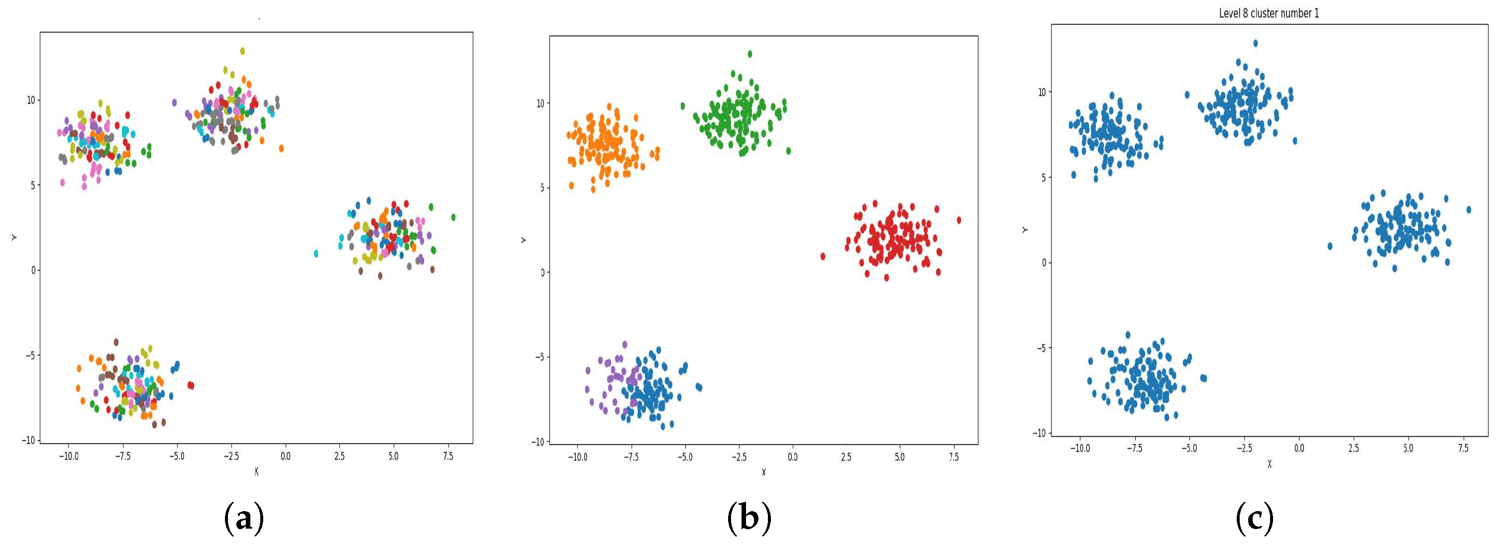
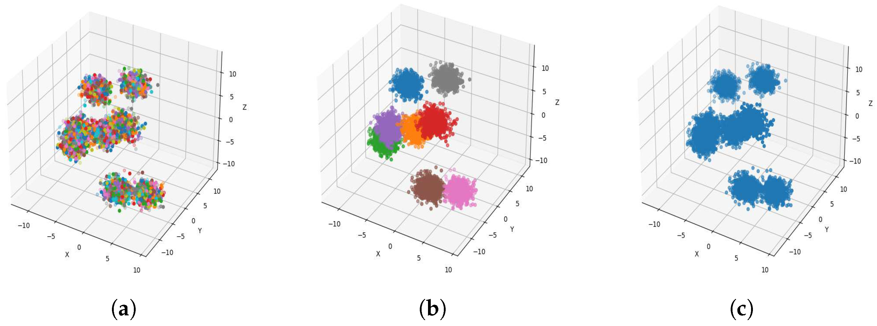
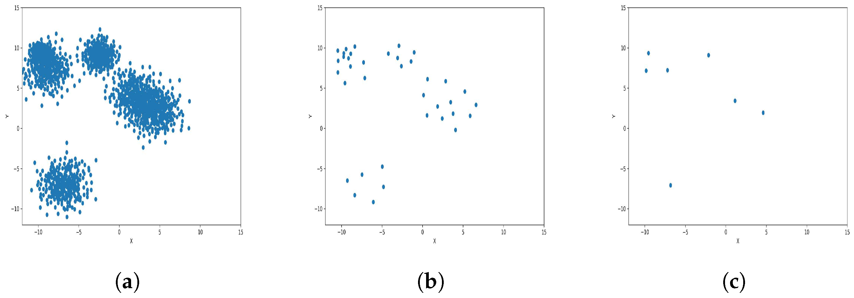
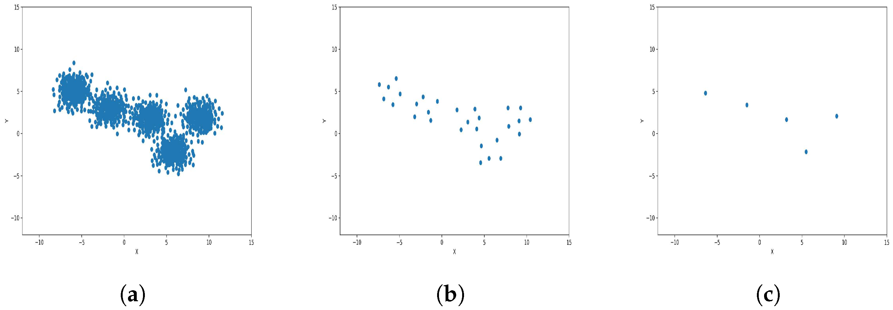
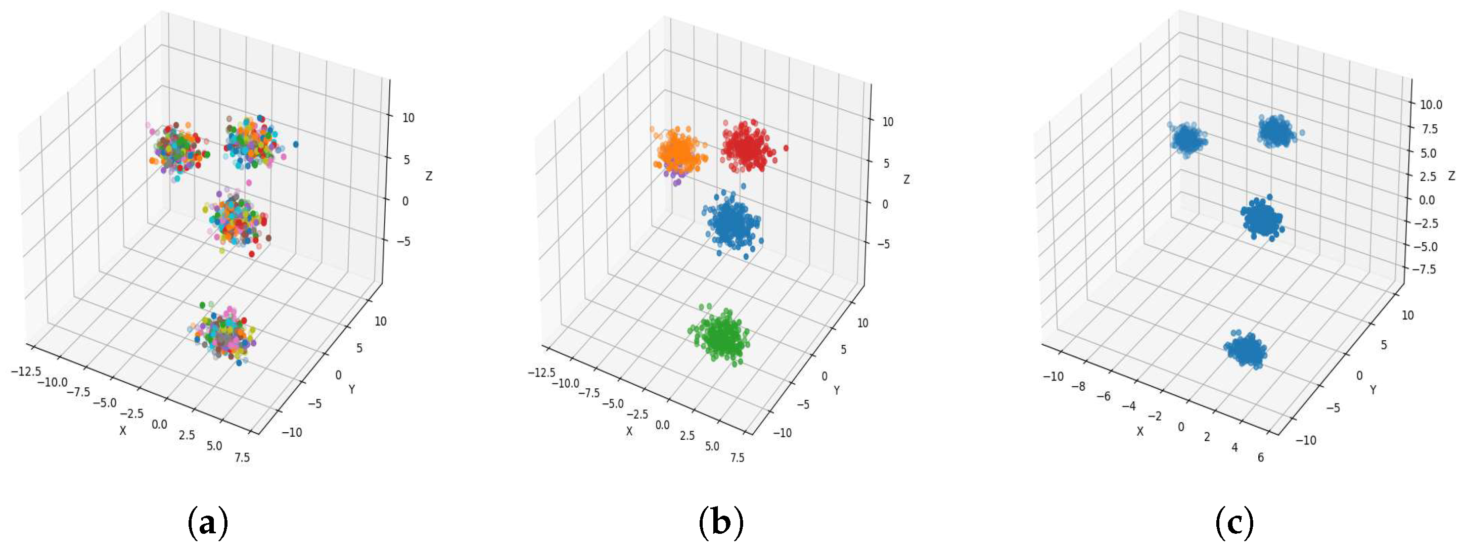
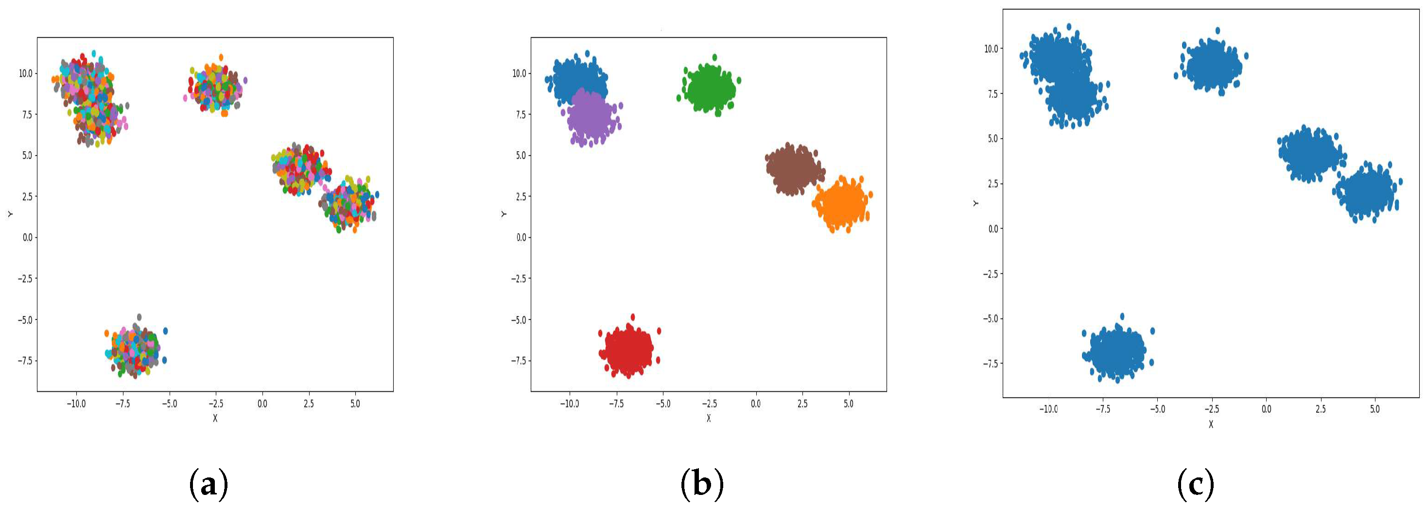
The proposed algorithm is implemented in Python (The code is available on GitHub [24]) on a personal computer with Intel^®, core ™i5-8550u, [email protected] GH, 8 GB laptop running Windows 10. To evaluate the performance of the proposed work, we applied the clustering algorithm to various synthetic datasets. Figure 4, Figure 5, Figure 6 and Figure 7 show the clustering results with different levels of clusters, varying dataset sizes, and different numbers of clusters.

Figure 4a, Figure 5a, Figure 6a and Figure 7a, show level 1, which begins by merging each cluster with its nearest neighbor cluster, resulting in fewer clusters. In level 2, the number of clusters further decreases as clusters are merged with their nearest neighbor clusters. In level 4, as illustrated in Figure 4b, Figure 5b, Figure 6b and Figure 7b, the number of clusters is observed to be equal to the number of groups from which the dataset is originally formed. This process continues iteratively at every level until all clusters are eventually combined into a single cluster, as shown in Figure 4c, Figure 5c, Figure 6c and Figure 7c. This observation underscores the correctness and accuracy of the algorithm in handling datasets with varying structures, including differences in the number of dimensions and the number of groups within the dataset.

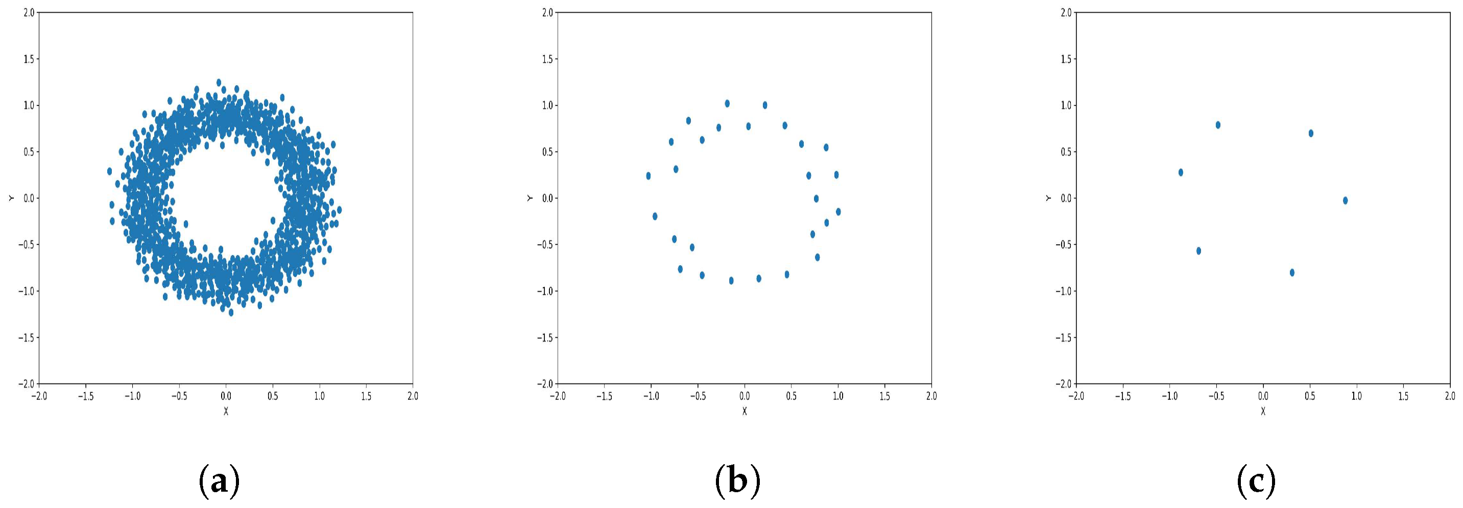
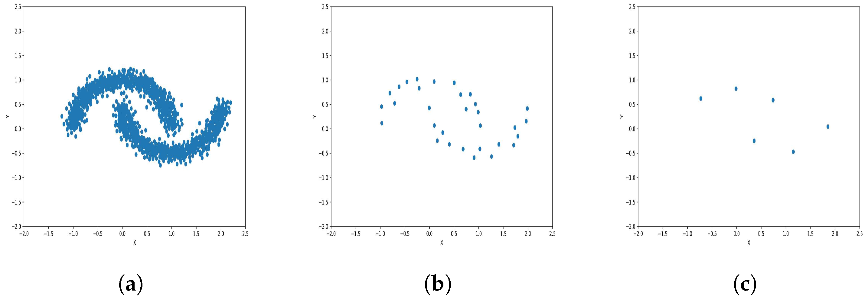
To reduce the dataset size required for machine learning and other applications, the K-level algorithm employs cluster centers to represent all elements within each cluster regardless of size. This allows it to represent the dataset without altering its overall meaning and distribution of elements within it. To illustrate this concept and elucidate its results, we applied the algorithm to six synthetic datasets featuring distinct data distributions, as depicted in Figure 8, Figure 9, Figure 10, Figure 11, Figure 12 and Figure 13.

The results observed in the figures reveal that, as the level of consolidation increases, the number of data points decreases while maintaining the shape and overall distribution of the elements. In level 6, as depicted in Figure 8c, Figure 9c, Figure 10c, Figure 11c, Figure 12c and Figure 13c, there are notably fewer points compared to the original dataset’s size. However, the general shape of the distribution remains discernible. Consequently, the resultant data points from different levels can effectively represent the entire dataset and be utilized in various applications, yielding results that closely resemble those obtained using the complete dataset.

4.2. Results and Discussion

To evaluate the validity and accuracy of the K-level algorithm, we conducted a comparative analysis against previously introduced techniques, including UPGMA [3], CLINK [4], UPGMC [11], SLINK [2], and K-means [25]. We used internal validation metrics: Silhouette Score (1) [26], Davies–Bouldin Index (2) [27], and Calinski–Harabasz Index (3) [28]. These metrics provide insights into the quality and performance of the clustering algorithms, enabling a comprehensive comparison and assessment of the proposed K-level algorithm with different types of datasets, as shown in

Table 2. Comparison of clustering algorithms on Blob dataset (the bold characters are the best values).

Method	Blob
	Silhouette Score	Davies–Bouldin Index	Calinski–Harabasz Index
K-level	0.61	0.50	12,868.1
UPGMA	0.64	0.45	11,889.9
CLINK	0.64	0.45	12,093.73
UPGMC	0.55	0.45	12,032.22
SLINK	0.36	0.67	2456.5
K-means	0.61	0.50	12,512.4

,

Table 3. Comparison of clustering algorithms on Circles dataset (the bold characters are the best values).

Method	Circles
	Silhouette Score	Davies–Bouldin Index	Calinski–Harabasz Index
K-level	0.38	0.66	4305.6
UPGMA	0.41	0.68	3223.7
CLINK	0.38	0.69	2671.0
UPGMC	0.43	0.67	3399.3
SLINK	$-0.22$	0.68	2.15
K-means	0.45	0.65	3853.2

,

Table 4. Comparison of clustering algorithms on Moon dataset (the bold characters are the best values).

Method	Moon
	Silhouette Score	Davies–Bouldin Index	Calinski–Harabasz Index
K-level	0.44	0.72	4807.3
UPGMA	0.39	0.84	3509.3
CLINK	0.38	0.84	3562.9
UPGMC	0.42	0.79	3894.3
SLINK	$-0.38$	1.89	1.23
k-means	0.44	0.79	4490.9

and

Table 5. Comparison of clustering algorithms on Spiral dataset (the bold characters are the best values).

Method	Spiral
	Silhouette Score	Davies–Bouldin Index	Calinski–Harabasz Index
K-level	0.52	0.48	8593.2
UPGMA	0.54	0.58	5064.9
CLINK	0.54	0.58	5064.9
UPGMC	0.54	0.58	5064.9
SLINK	0.31	0.51	3.3
k-means	0.56	0.61	8871.9

.

The K-level clustering algorithm exhibits competitive performance compared to other clustering algorithms across different datasets. In the remainder of this subsection, we discuss the K-level results in comparison to other algorithms.

In the Blob dataset, K-level displays a solid Silhouette score of $0.61$, indicating well-defined clusters. The Davies–Bouldin Index, at $0.50$, confirms good cluster separation and pattern capture. Particularly noteworthy is the K-level’s outperformance of UPGMA and CLINK in the Calinski–Harabasz index, scoring 12,868.1 versus 11,889.9. This superiority in the Calinski–Harabasz index underscores the K-level’s ability to create distinct clusters in the Blob Dataset, highlighting its potential as a robust clustering method for this scenario. Therefore, K-level is well-suited for datasets with compact and separated clusters, making it an effective choice for problems where distinct, non-overlapping groups need to be identified.

In the Circles dataset, K-level exhibits a lower Silhouette score of 0.38, and the Davies–Bouldin index one of 0.66, which indicates relatively weaker cluster separation. However, the K-level performs reasonably well with a Calinski–Harabasz index of 4305.6, indicating some degree of cluster differentiation. Despite a slightly lower Silhouette score compared to UPGMA and CLINK (0.38 vs. 0.41), K-level compensates by surpassing them in the Calinski–Harabasz index (4305.6 vs. 3223.7), highlighting its potential to uncover patterns within the Circles dataset. For that, K-level is suitable for datasets with less distinct clusters, making it a viable option for problems where clusters may have some degree of overlap or a more complex arrangement.

In the Moon dataset, K-level impressively achieves a Silhouette score of $0.44$, indicating well-defined clusters. Moreover, it boasts a Davies–Bouldin Index of $0.72$, affirming robust cluster separation and pattern capture. Notably, K-level outperforms UPGMA and CLINK, recording a significantly higher Calinski–Harabasz index of $4807.3$ compared to their scores of $5064.9$. This superior performance in the Calinski–Harabasz index highlights K-level’s proficiency in generating well-defined clusters, establishing it as a strong clustering method for the Moon dataset. In summary, K-level is suitable for problems wherein the dataset contains well-separated clusters with clear boundaries, making it effective in scenarios requiring precise cluster identification.

In the Spiral dataset, K-level demonstrates moderate clustering quality with a Silhouette score of $0.52$. Additionally, it excels in cluster separation, as evidenced by a Davies–Bouldin index of $0.48$. The high Calinski–Harabasz index of $8593.2$ signifies well-defined clusters. While K-level’s Silhouette score is comparable to UPGMA and CLINK ($0.52$ vs. $0.54$), it surpasses them with a superior Calinski–Harabasz index ($8593.2$ vs. $5064.9$), emphasizing its ability to yield more distinct clusters in the Spiral dataset and establishing it as an effective clustering method for this dataset. As a result, K-level is suitable for datasets where clusters may not be as compact but still exhibit discernible patterns, making it a good choice for problems wherein clusters have varying shapes and sizes.

The observed results from various datasets demonstrate that the K-level algorithm’s specific characteristics such as precise distance measurement, fitness criteria, greedy merging, hierarchical structure formation, and adaptive clustering levels allow it to effectively identify and merge the closest clusters, contributing to well-defined clusters in the Blob and Moon datasets, as shown by high Silhouette scores and Calinski–Harabasz index values. Considering the intra-cluster similarity and inter-cluster separation, the fitness criteria ensure robust performance, evidenced by the Davies–Bouldin index values indicating good separation, particularly in the Blob and Spiral datasets. The greedy merging process maintains computational efficiency and scalability, reflected in moderate-to-high Calinski–Harabasz index values. The hierarchical structure formation manages complex datasets with varying shapes, benefiting the Moon and Spiral datasets. Additionally, allowing users to specify the number of clusters to merge at each level provides enhanced control, ensuring adaptability and effective clustering, as seen in the Circles dataset.

The K-level clustering algorithm demonstrates strong performance when clusters are well-separated, as indicated by high Silhouette scores and low Davies–Bouldin index values. Additionally, it always outperforms UPGMA and CLINK in the Calinski–Harabasz index, highlighting its ability to create clusters that maximize inter-cluster variance relative to intra-cluster variance. This algorithm is well-fit for scenarios requiring distinct cluster identification, excelling in tasks where the goal is to identify well-defined, non-overlapping clusters. Furthermore, its effectiveness extends to datasets with different cluster structures. In summary, it proves that K-level appears as a versatile clustering algorithm, indicating effectiveness in scenarios characterized by well-defined and separated clusters, as well as being particularly suitable for problems involving different cluster shapes and sizes.

4.3. Complexities Analysis

This section provides the complexity analysis of the K-level algorithm, encompassing both time and space complexities. Several key factors depend on the time complexity of the algorithm. In each iteration over the k levels, the m clusters merge, and the original size of the dataset n, the algorithm, for each cluster x in $C_i$, constructs the distance array $D\left(x\right)$ by calculating Euclidean distances to other clusters. The process of selecting m clusters with the smallest distances and merging them into a new cluster also has a time complexity of $O\left(n\right)$, involving searching through the distance array and updating the merged cluster. Consequently, the loop for each cluster x in $C_i$ has a time complexity of $O(n/m)$. Furthermore, the complexity of the distance array $D\left(x\right)$ is $O(n/m)$. The operation of merging m clusters into a single cluster has a time complexity of $O(n/m)$. The outer loop runs k times, and each iteration involves steps 1–3. Therefore, the overall time complexity is $O(k·(n/m)·(n/m)·(n/m\left)\right)$, where k is a static number, leading to a simplified time complexity of $O(n^3/m^3)$.

The time complexity is influenced by the number of levels k, the size of the dataset n, and the number of clusters merged simultaneously m. Increasing m reduces the number of iterations needed, thereby reducing the overall time complexity. This characteristic reflects the algorithm’s structure, where merging more clusters per iteration leads to fewer total iterations, enhancing computational efficiency.

On the other hand, the space complexities of the K-level algorithm depend on the size of the $C_i$ array. In each iteration at level k, the algorithm utilizes the $C_i$ array without the use of any other array. Therefore, the space complexity of K-level is $O\left(n\right)$, where n is the size of the original dataset. The space complexity is primarily influenced by the need to store the cluster sets and the distance arrays. The algorithm efficiently uses memory by maintaining only the necessary data structures at each level, without requiring additional storage for intermediate computations. This characteristic demonstrates the algorithm’s efficient memory utilization, making it suitable for large datasets.

Based on

Table 6. Comparison of the time and memory complexities for clustering algorithms (n is the size of the dataset, m number of clusters to merge simultaneously).

Method	Time Complexity	Memory Complexity
K-level	$O(n_3/m_3)$	$O\left(n\right)$
UPGMA	$O\left(n_3\right)$	$O\left(n_2\right)$
CLINK	$O\left(n_3\right)$	$O\left(n_2\right)$
UPGMC	$O\left(n_3\right)$	$O\left(n_2\right)$
SLINK	$O\left(n_3\right)$	$O\left(n_2\right)$
Median-link	$O\left(n^3\right)$	$O\left(n^2\right)$

, K-level demonstrates lower time complexity compared to traditional hierarchical clustering algorithms, including UPGMA, CLINK, UPGMC, SLINK, and Median-link. In particular, the time complexity for K-level is expressed as $O(n_3/m_3)$, contrasting with the $O\left(n_3\right)$ time complexity common to the other algorithms. When the value of m increases, the time complexity of K-level decreases.

K-level exhibits a favorable memory complexity, denoted as $O\left(n\right)$. This memory complexity is notably lower compared to the other clustering algorithms listed in Table 6. The efficient memory utilization of K-level makes it a promising choice, especially in scenarios where minimizing memory usage is crucial and in large datasets.

4.4. Time Consumption Analysis

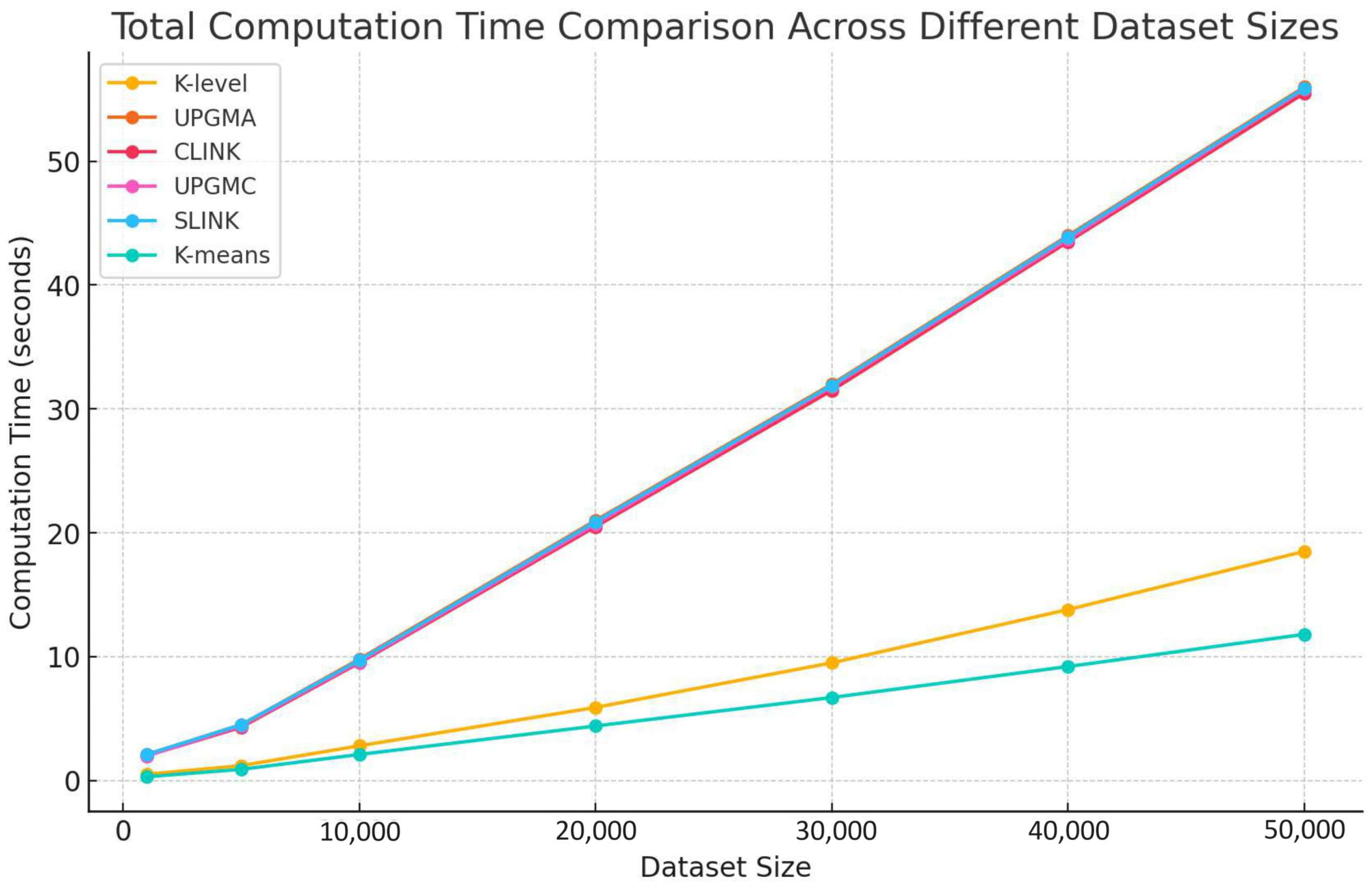
In this subsection, we analyze the total computation time across different dataset sizes for various clustering algorithms, including UPGMA, CLINK, UPGMC, SLINK, and K-means, as illustrated in Figure 14.

Our comparison reveals significant differences in computation time among the clustering algorithms as dataset sizes increase. The K-level algorithm demonstrates the least computation time across all dataset sizes. On the other hand, traditional hierarchical algorithms, namely UPGMA, CLINK, UPGMC, and SLINK, show marked increases in computation time as dataset sizes expand, reflecting their higher computational complexities. The similarity in computation time between the K-level algorithm and K-means suggests a moderate increase in computation time, which enhances its efficiency compared to traditional hierarchical methods.

The K-level algorithm’s superior performance, in terms of computation time across various dataset sizes, highlights its lower computation demands and better scalability relative to traditional hierarchical methods. This performance validates the design and efficiency of the K-level algorithm, positioning it as a robust and efficient clustering solution for handling large-scale datasets. Such characteristics make the K-level algorithm particularly suitable for modern data-intensive applications, emphasizing its potential for broad adoption in real-world scenarios where processing efficiency and scalability are paramount.

4.5. Applications in Wireless Sensor Networks

The proposed K-level clustering algorithm, with its nature-inspired design and efficient hierarchical structure formation, is particularly well-suited for various real-world applications in wireless sensor networks (WSNs). This section explores the potential applications of the K-level algorithm in different WSN-based scenarios, highlighting its adaptability and efficiency.

4.5.1. Environmental Monitoring

In environmental monitoring, WSNs are deployed to collect data on various environmental parameters such as temperature, humidity, air quality, and pollution levels. The K-level algorithm can significantly enhance the efficiency of data aggregation and clustering in several ways. First, through hierarchical data aggregation, the K-level algorithm clusters sensor nodes based on their proximity and data similarity, creating hierarchical structures that facilitate efficient data aggregation and reduce communication overhead. Additionally, the K-level algorithm supports scalable monitoring. Since environmental monitoring often involves large-scale deployments, the algorithm’s ability to handle extensive datasets within a reasonable timeframe ensures that the monitoring system remains scalable and responsive.

4.5.2. Precision Agriculture

Precision agriculture leverages WSNs to monitor soil moisture, nutrient levels, and crop health, enabling farmers to make data-driven decisions. The K-level algorithm can be applied to optimize these monitoring processes in several ways. Through adaptive clustering, the algorithm can adapt to varying data types collected from different sensors (e.g., soil moisture, temperature, and humidity) and cluster them efficiently, providing a comprehensive view of the agricultural field. Additionally, by reducing the amount of data transmitted through the network, the K-level algorithm helps conserve the energy resources of sensor nodes, thereby extending the network’s operational lifetime.

4.5.3. Health Monitoring

WSNs are increasingly used in health monitoring systems to track patients’ vital signs and activity levels. The K-level algorithm can improve these systems in several ways. First, through personalized health data clustering, the algorithm can cluster health data from multiple sensors worn by patients, helping to identify patterns and anomalies in vital signs, which facilitates early diagnosis and personalized healthcare. Additionally, the algorithm supports scalable patient monitoring. In large healthcare facilities, it can scale to monitor numerous patients simultaneously, ensuring efficient data handling and real-time monitoring.

4.5.4. Smart Cities

Smart city applications use WSNs for a range of services, including traffic monitoring, waste management, and energy consumption tracking. The K-level algorithm can enhance these services in several ways. Through dynamic clustering, the K-level algorithm can, for example, dynamically cluster sensor nodes based on real-time traffic conditions, enabling more accurate and timely traffic management and control. Additionally, the algorithm optimizes data processing for waste management by clustering data from sensors placed in waste bins across the city, thus optimizing collection routes and schedules based on the fill levels and locations of the bins.

The K-level clustering algorithm offers a robust and scalable solution for various applications in WSNs, addressing the challenges of data volume, dimensionality, and complex data structures. Its efficient hierarchical clustering and adaptive capabilities make it suitable for a wide range of realistic scenarios, from environmental monitoring and precision agriculture to smart cities, health monitoring, and industrial automation. By leveraging the K-level algorithm, WSN-based systems can achieve enhanced performance, scalability, and efficiency, contributing to the advancement of these critical applications.

5. Conclusions

This article proposes a new nature-inspired clustering algorithm K-level, which presents a significant advancement in addressing the limitations associated with traditional hierarchical clustering algorithms. The algorithm efficiently utilizes computation and memory resources, offering a novel approach to hierarchical clustering by merging based on distances in stages. Unlike traditional linkage algorithms, the K-level algorithm’s usefulness is also demonstrated by its capability to handle various data types. Additionally, it facilitates the generation of new data with characteristics and patterns similar to the original dataset. Furthermore, a comparative analysis against other clustering algorithms demonstrates its superiority by variant internal validation metrics. Additionally, our proposed K-level algorithm has a lower time and space complexity. These findings validate that our algorithm suits problems involving different cluster shapes and sizes. In future research, we intend to evaluate the K-level algorithm on real-world datasets from various domains, such as bioinformatics and social network analysis. We will explore extending the K-level algorithm to dynamic and online clustering scenarios, adapting it for streaming data where the clustering structure needs real-time updates. Additionally, we will investigate optimizing the algorithm’s parameters, like the number of clusters to merge at each level (m). Combining the K-level algorithm with other clustering techniques, such as density-based or model-based, could yield hybrid approaches, enhancing clustering accuracy and handling of more complex data structures.