Hybrid Adaptive Impedance and Admittance Control Based on the Sensorless Estimation of Interaction Joint Torque for Exoskeletons: A Case Study of an Upper Limb Rehabilitation Robot

Abstract

Physiotherapy is the treatment to recover a patient’s mobility and limb function after an injury, illness, or disability. Rehabilitation robots can be used to replace human physiotherapists. To ensure safety during robot physical therapy, the patient’s limb needs to be controlled to track a desired joint trajectory, and the torque due to interaction force/torque needs to be measured and regulated. Therefore, hybrid impedance and admittance with position control (HIPC) is required to track the trajectory and simultaneously regulate the contact torque. The literature describes two structures of HIPC: (1) a switched framework between admittance and impedance control operating in parallel (HIPCSW); and (2) a series connection between admittance and impedance control without switching. In this study, a hybrid adaptive impedance and position-based admittance control (HAIPC) in series is developed, which consists of a proportional derivative-based admittance position controller with gravitational torque compensation and an adaptive impedance controller. An extended state observer is used to estimate the interaction joint torque due to human stiff contact with the exoskeleton without the use of force/torque sensor, which is then used in the adaptive algorithm to update the stiffness and damping gains of the adaptive impedance controller. Simulation results obtained using MATLAB show that the proposed HAIPC significantly reduces the mean absolute values of the actuation torques (control inputs) required for the shoulder and elbow joints in comparison with HIPC and HIPCSW.

1. Introduction

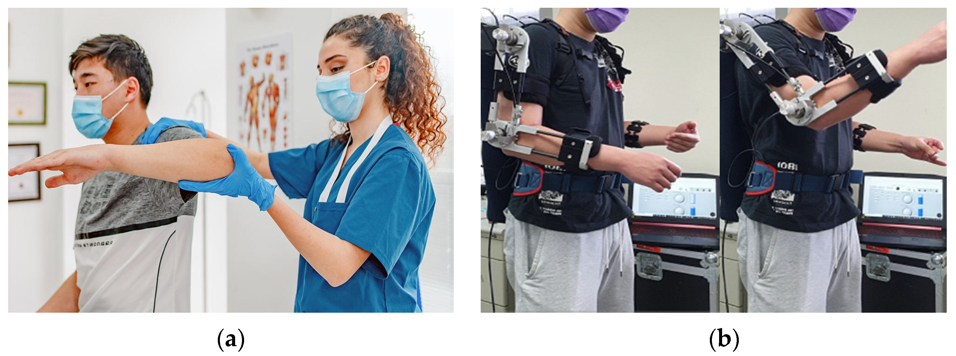
Physical therapy is a process whereby patients undergo rehabilitation to recover limb functionality and arm mobility after stroke or injury. Usually, physiotherapist doctors help patients to carry out physical therapy, as shown in Figure 1a. However, with developments in neuroengineering research, rehabilitation robots can be used to replace human physiotherapists, as shown in Figure 1b. Safe close-proximity human [1,2] and exoskeleton [3,4] interactions with robots can be achieved through two complementary strategies: (1) using smart actuators [5] with adjustable intrinsic properties, e.g., stiffness [6] and damping [7], and (2) by impedance control [8,9]. Impedance control provides safe and stable robot–environment interaction. The two main types of interaction controls that are widely used in robotics are impedance control, in which the input is either position or velocity and the output is force/torque, and admittance control, which is the opposite of impedance control [10]. During physical therapy with doctors, the physiotherapist controls the motion and regulates the interaction joint torque for safe movement with the patient’s arms [11]. Similarly, when a robotic manipulator makes contact with the environment (e.g., human) as shown in Figure 1b, controlling both the interaction force/torque and its motion is needed because human–robot interactions can be hazardous if safety is not considered [12,13]. Generally, when a robot interacts with a stiff environment, impedance control is more stable than admittance control, while the reverse applies when the robot interacts with a soft or free-space environment. However, if the robot interacts with an unknown environment or an environment with varying mechanical characteristics (i.e., stiff and soft properties at different points), it is difficult to choose between impedance control or admittance control application. In this case, a hybrid between impedance control and admittance with position control might yield more satisfactory results. Basically, there are two types of force control: admittance control (usually with a position controller such as PID/PD, fuzzy, and sliding mode) and impedance control. Admittance control with a position controller can only control the position and force without monitoring the manipulator’s impedance, whereas impedance control can regulate the interaction force/torque by monitoring the impedance. Therefore, a hybrid impedance control was proposed to combine the two fundamental force controls to simultaneously control both the position and interaction force/torque [14].

Figure 1. (a) Physical therapy with doctor [11] and (b) physical therapy with rehabilitation robot [13].

The literature presents two structures for hybrid impedance position control (HIPC). The first and most-used method is a parallel connection of the admittance with position control and impedance control, or, in some studies, only the position controller and impedance control. In this structure (hereafter HIPCSW), a switching mechanism is used to activate either the admittance or impedance controller at any given instant. Switching between the controllers is usually determined based on the nature of the environment: if the environment is soft, the admittance position controller is activated; if the environment is stiff, the impedance controller is activated. However, there are two main limitations in this switched framework. First, the knowledge of the nature of the environment must inform switching between admittance and impedance control. Second, there is a problem in designing the switching mechanism, as it may cause discontinuity in the control input if switching is not sufficiently fast, or it may result in chattering if the switching speed is too fast.

2. Related Work

This section presents some related work based on the two structures of hybrid impedance control. A discussion on the parallel structure with a switching mechanism, a series structure without the switching mechanism, an interaction joint torque sensorless estimation, and a conclusion will be provided.

2.1. Parallel Structure with a Switched Framework

Some related studies on the parallel framework with the switching mechanism have been reported. For example, a pioneering study [14] introduced hybrid impedance control, which is a hybrid between a position controller and an impedance controller combined in parallel and implemented within a single framework. Since the publication of reference [14], several other designs of hybrid impedance controls have been proposed, such as in reference [15], where the controllers are connected in parallel via a switch (i.e., HIPCSW). The switching occurs based on the nature of the environment to either admittance control for soft or noncontact environments and impedance for stiff environments. The switching mechanism was based on the duty cycle and switching period. A robust hybrid impedance control was developed [16], where the computed torque is applied in a hybrid with a PI controller for the regulation of torque and position tracking. An earlier study [17] developed a hybrid impedance control strategy that combines impedance and position control into one strategy for the rehabilitation of a patient’s wrist and forearm. Another study [18] proposed a hybrid impedance control where the controller concurrently achieves position motion tracking for rehabilitation and produces a force using an optimization process based on a musculoskeletal model. Recently, a hybrid impedance control mechanism for optimal environmental–robot interaction was presented in [19,20], which proposed an improved hybrid impedance control for variable stiffness environment interaction. Other parallel structured hybrid impedance control methods have been proposed elsewhere [21,22,23,24,25,26,27,28]. Adaptive hybrid impedance control was also proposed in [29,30,31,32,33].

2.2. Series Structure without a Switched Framework

The second structure is a series hybrid connection between admittance position control and impedance control. This framework [34] employs no switch, but the two controllers are combined to generate the control signal based on the proportion. Depending on the mechanical nature of the environment, a weighting factor is used to determine which controller is more dominant. When the environment is soft, the admittance position control contributes a greater percentage of the control signal, and when the environment is stiff, the impedance control prevails. Recently, reference [35] proposed a new hybrid impedance control without switching. The design is simulated and implemented on a two-dimensional manipulator. Herein, the admittance controller is connected in series with both the position controller and the impedance controller. The admittance controller generates a new desired trajectory when an external force/torque is applied. The new trajectory is used by the position controller and the impedance controller to respond to changes due to external contact force/torque. Impedance control regulates the interaction force to achieve robot compliance with different types of environmental properties. However, the magnitude of the interaction force/torque is unknown, and its values depend on inertia, damping, and the stiffness of the environment. Because in most cases, the actual values of inertia, damping, and stiffness are difficult to determine, the magnitude of the interaction force/torque can be estimated or measured using a force/torque sensor.

2.3. Interaction Force/Torque Sensorless Estimation

Most industrial robots come without embedded force/torque sensor(s). Incorporating such a force/torque sensor incurs extra cost. Visual servo control [36] is a promising alternative for manipulation but does not provide a complete perception of interaction force. To avoid the use of sensors, different methods have been proposed to estimate the interaction force/torque, e.g., extended Kalman filters [37,38,39,40,41], adaptive Kalman filters [42], extended state observers [43,44,45,46,47,48,49,50], disturbance observers [51,52], nonlinear observers [53], deep neural networks [54], model-based compensation techniques [55,56], task-oriented models based on dynamic model learning and a robust disturbance state observer [57], a sensorless force estimation method using a disturbance observer and the neural learning of friction [58], and extended Kalman filters [59].

2.4. Conclusion

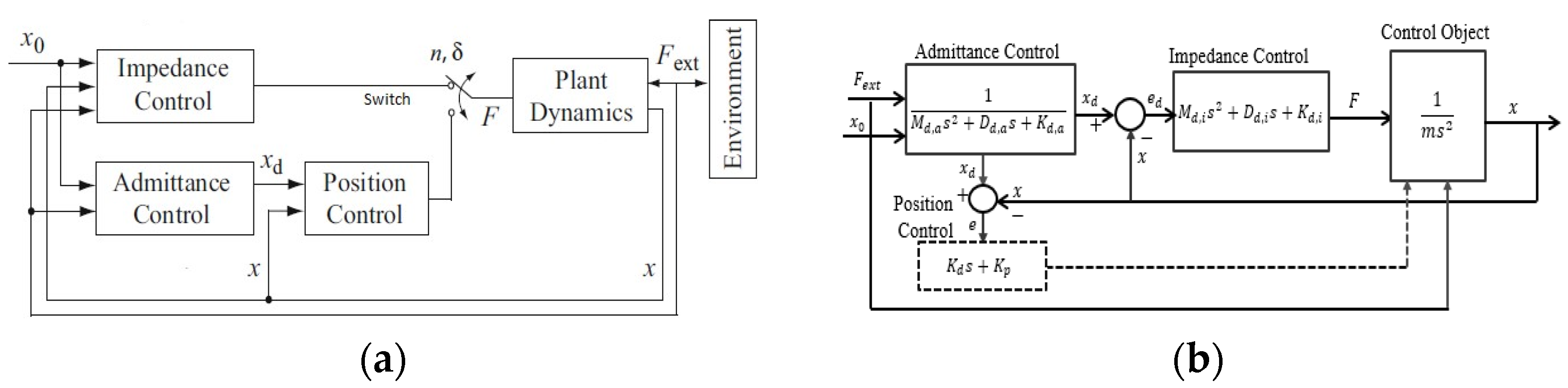
Based on the above review of the literature, most of the hybrid impedance controls are based on parallel connections between the two force controllers using a switch (HIPCSW), as shown in Figure 2a. However, the switching process between the controllers must be fast enough to avoid the discontinuity of the control signal, which can lead to unstable behavior. In addition, the switching process is based on a desired switching frequency and duty ratio, and in some studies, a selection matrix is used for the switching mechanism, i.e., the mechanical properties of the environment must be known a priori to correctly adjust the duty ratio or selection matrix in advance to switch to the appropriate controller at the time of contact. Meanwhile, the HIPC with a series connection between the two force controllers without switching [35], as shown in Figure 2b, uses high fixed stiffness and damping gains, which consume high control torque. Therefore, in this work, a hybrid adaptive impedance and position-based admittance control (HAIPC) is proposed to further improve the performance in reducing the control torque. A comparison between the control structures is given in Table 1.

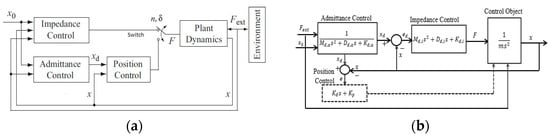
Figure 2. (a) Parallel structure HIPCSW [15]: the impedance and admittance controls are connected in parallel via a switch. (b) Series structure HIPC [35]: the impedance and admittance controls are connected in series.

Table 1. Comparison of the major differences between the related works.

Control Methods	Advantages	Disadvantages
Parallel Structure (i.e., HIPCSW)	Low starting control input torque. Only one controller produced the control signal at a time depending on the nature of contact. Admittance for soft contact and impedance for stiff contact.	Additional cost of switching mechanism. Control input discontinuity if the switch is slow leading to instability. Control signal chattering if the switch is fast. High total control input torque due to chattering.
Series Structure (i.e., HIPC)	No additional cost of switching mechanism. No discontinuity or chattering in the control input. Low total control input torque.	High starting control input torque. Both admittance and impedance controls together produced the control signal during soft and stiff contact.

2.5. Research Contributions

The proposed method combined the impedance and admittance controllers in series without switching to avoid possible instability and chattering. Similarly, the mechanical properties of the environment need not be known using HAIPC. However, for upper limb rehabilitation robots, the damping and stiffness of the contact force/torque not only depend on the moving posture but also differ from one patient to another depending on the stage of patient recovery. Hence, the performance of impedance control can be improved if the damping and stiffness adapt to the estimated patient’s interaction joint torque. Therefore, in this study, the interaction joint torque is estimated to update the stiffness and damping in hybrid adaptive impedance control. Hence, the system will adapt based on the magnitude of the estimated interaction joint torque, which varies from patient to patient. The proposed control method has advantages as follows: Adaptive impedance generates almost zero torque when the environment is soft and only increases to a high torque value when stiff contact is made between the human and the robot. In addition, feedforward gravitational compensation is added to the position-based admittance control to improve transparency against the effect of resistance from gravity, thereby reducing the effort needed from the patient to reach the desired position during the rehabilitation exercise at any point away from the equilibrium. Furthermore, the proposed control consumes less control torque, which allows the use of more compact actuators with a lower gear ratio and higher back drivability. The contributions of this work to the existing related work can be summarized as follows:

• The proposed method used the sensorless estimated interaction joint torque based on the actuator input torque of the system to update the stiffness and damping constants in the impedance control. This implies that the control torque due to impedance control is zero during soft contact, unlike the HIPC, which has high constant stiffness and damping gains both during soft and stiff contacts. Thus, the proposed method has low starting control input torque.
• The proposed method is adaptive and is designed based on series structure to avoid possible instability and chattering due to the switching process. Therefore, it combines the advantages of both HIPCSW and HIPC, namely low starting control input torque, the avoidance of instability and chattering effects, and low total control input torque consumption.
• To the best of our knowledge, based on the literature review, the proposed method is the first to use the sensorless estimation of interaction joint torque in the adaptive algorithm to update the stiffness and damping constant in the impedance control.

3. Mathematical Modelling

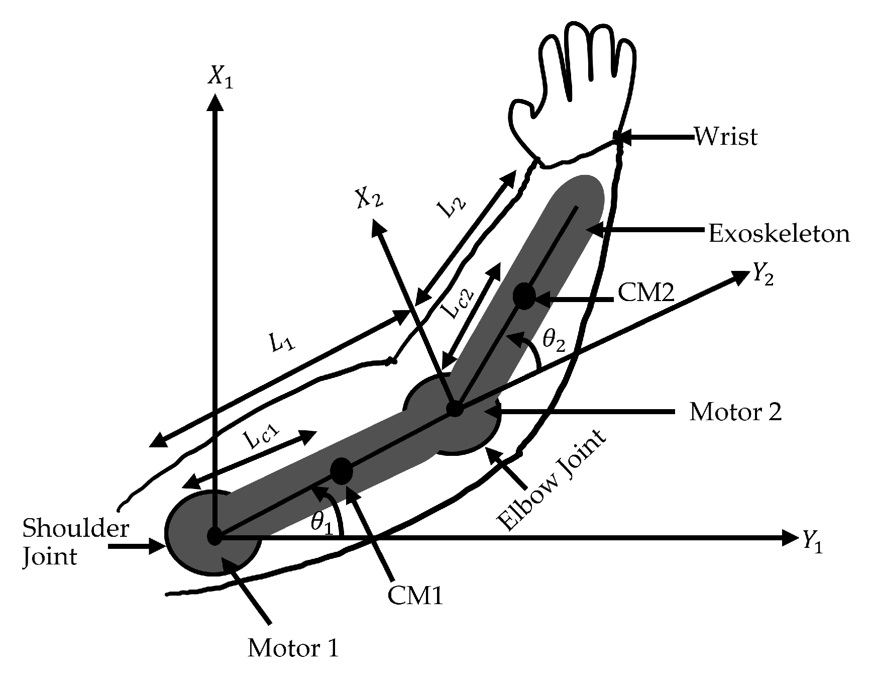
The dynamic model is derived for simulation purposes. HAIPC is compared with the HIPC and HIPCSW using the same dynamic model of the upper extremity exoskeleton shown in Figure 3.

Figure 3. Schematic diagram of 2DOF upper-extremity exoskeleton for rehabilitation: $L_1$ and $L_2$ represent the distance from the shoulder to the elbow joints and the distance from the elbow to the wrist joints. $L_{c1}$ and $L_{c2}$ represent the distance from the shoulder joint to the arm’s center of mass CM1 and the distance from the elbow joint to the arm’s center of mass CM2. ${\theta }_1$ and ${\theta }_2$ represent the shoulder joint and elbow joint angular displacements. Motor 1 and motor 2 represent the joint actuators of the exoskeleton.

Nonlinear Model

The dynamic model of the system used in this study is derived from [60]. Figure 3 illustrates the upper limb wearable rehabilitation robot used, where $L_1$ and $L_2$ represent the lengths of the upper arm and lower arm. The distances between the upper arm and lower arm’s centers of mass and the shoulder and elbow joint’s center are described by $L_{c1}$ and $L_{c2}$, and ${\theta }_1$ and ${\theta }_2$ represent the shoulder joint and elbow joint angular displacements, respectively. Table 2 gives the values of the system’s parameters.

Table 2. Parameters of the system [60].

Parameters	Symbols	Values	Units
Mass of the Upper Arm Limb	$m_1$	2.25	kg
Mass of the Lower Arm Limb	$m_2$	1.47	kg
Upper Arm Length	$L_1$	0.34	m
Lower Arm Length	$L_2$	0.25	m
Distance from Shoulder to Upper Arm CM	$L_{c1}$	0.17	m
Distance from Elbow to Lower Arm CM	$L_{c2}$	0.125	m
Mass Moment of Inertia about the Shoulder Joint	$I_1$	0.2505	kg × m2
Mass Moment of Inertia about the Elbow Joint	$I_2$	0.0925	kg × m2

The dynamic model of the 2DOF upper extremity exoskeleton system is generally represented as follows:

$$\mathit{M}\left(\mathit{\theta }\right)\ddot{\mathit{\theta }}+\mathit{C}\left(\mathit{\theta },\dot{\mathit{\theta }}\right)\dot{\mathit{\theta }}+\mathit{G}\left(\mathit{\theta }\right)=\left[\begin{array}{c}{\mathit{\tau }}_{\mathit{s}}\\ {\mathit{\tau }}_{\mathit{e}}\end{array}\right]$$

(1)

where $\mathit{M}\left(\mathit{\theta }\right)$, $\mathit{C}\left(\mathit{\theta },\dot{\mathit{\theta }}\right)$, $\mathit{G}\left(\mathit{\theta }\right)$, ${\mathit{\tau }}_{\mathit{s}}$, and ${\mathit{\tau }}_{\mathit{e}}$ are the mass/moment of inertia of the links and motors matrix, C is the centrifugal and Coriolis force, and G contains the gravitational terms, shoulder control torque, and elbow control torque. The matrices are given as follows:

$$\mathit{M}\left(\mathit{\theta }\right)\ddot{\mathit{\theta }}=\left[\begin{array}{cc}{\mathit{I}}_{\mathbf{1}}+{\mathit{I}}_{\mathbf{2}}+{\mathit{m}}_{\mathbf{1}}{\mathit{L}}_{\mathit{c}\mathbf{1}}^{\mathbf{2}}+{\mathit{m}}_{\mathbf{2}}\left({\mathit{L}}_{\mathbf{1}}^{\mathbf{2}}+{\mathit{L}}_{\mathit{c}\mathbf{2}}^{\mathbf{2}}+\mathbf{2}{\mathit{L}}_{\mathbf{1}}{\mathit{L}}_{\mathit{c}\mathbf{2}}\mathbf{cos}\left({\mathit{\theta }}_{\mathbf{2}}\right)\right)& {\mathit{I}}_{\mathbf{2}}+{\mathit{m}}_{\mathbf{2}}\left({\mathit{L}}_{\mathit{c}\mathbf{2}}^{\mathbf{2}}+\mathbf{2}{\mathit{L}}_{\mathbf{1}}{\mathit{L}}_{\mathit{c}\mathbf{2}}\mathbf{cos}\left({\mathit{\theta }}_{\mathbf{2}}\right)\right)\\ {\mathit{I}}_{\mathbf{2}}+{\mathit{m}}_{\mathbf{2}}\left({\mathit{L}}_{\mathit{c}\mathbf{2}}^{\mathbf{2}}+\mathbf{2}{\mathit{L}}_{\mathbf{1}}{\mathit{L}}_{\mathit{c}\mathbf{2}}\mathbf{cos}\left({\mathit{\theta }}_{\mathbf{2}}\right)\right)& {\mathit{I}}_{\mathbf{2}}+{\mathit{m}}_{\mathbf{2}}\left({\mathit{L}}_{\mathit{c}\mathbf{2}}^{\mathbf{2}}\right)\end{array}\right]$$

(2)

$$\mathit{C}\left(\mathit{\theta },\dot{\mathit{\theta }}\right)=\left[\begin{array}{cc}-\mathbf{2}{\mathit{m}}_{\mathbf{2}}{\mathit{L}}_{\mathbf{1}}{\mathit{L}}_{\mathbf{2}}{\dot{\mathit{\theta }}}_{\mathbf{2}}\mathbf{sin}\left({\mathit{\theta }}_{\mathbf{2}}\right)& -\mathbf{2}{\mathit{m}}_{\mathbf{2}}{\mathit{L}}_{\mathbf{1}}{\mathit{L}}_{\mathbf{2}}{\dot{\mathit{\theta }}}_{\mathbf{2}}\mathbf{sin}\left({\mathit{\theta }}_{\mathbf{2}}\right)\\ \mathbf{2}{\mathit{m}}_{\mathbf{2}}{\mathit{L}}_{\mathbf{1}}{\mathit{L}}_{\mathbf{2}}{\dot{\mathit{\theta }}}_{\mathbf{1}}\mathbf{sin}\left({\mathit{\theta }}_{\mathbf{2}}\right)& \mathbf{0}\end{array}\right]$$

(3)

$$\mathit{G}\left(\mathit{\theta }\right)=\left[\begin{array}{c}{\mathit{m}}_{\mathbf{1}}\mathit{g}{\mathit{L}}_{\mathit{c}\mathbf{1}}\mathbf{cos}\left({\mathit{\theta }}_{\mathbf{1}}\right)+{\mathit{m}}_{\mathbf{2}}\mathit{g}\left({\mathit{L}}_{\mathbf{1}}\mathbf{cos}\left({\mathit{\theta }}_{\mathbf{1}}\right)+{\mathit{L}}_{\mathit{c}\mathbf{2}}\mathbf{cos}({\mathit{\theta }}_{\mathbf{1}}+{\mathit{\theta }}_{\mathbf{2}}\right))\\ {\mathit{m}}_{\mathbf{2}}\mathit{g}{\mathit{L}}_{\mathit{c}\mathbf{2}}\mathbf{cos}\left({\mathit{\theta }}_{\mathbf{1}}+{\mathit{\theta }}_{\mathbf{2}}\right)\end{array}\right]$$

(4)

By substituting $\mathit{M}\left(\mathit{\theta }\right)$, $\mathit{C}\left(\mathit{\theta },\dot{\mathit{\theta }}\right)$, and $\mathit{G}\left(\mathit{\theta }\right)$ into Equation (1) and decoupling the system into shoulder and elbow equations separately, the following are obtained:

$$\begin{array}{ll}{\mathit{\tau }}_{\mathit{s}}=({\mathit{I}}_{\mathbf{1}}+{\mathit{I}}_{\mathbf{2}}+& {\mathit{m}}_{\mathbf{1}}{\mathit{L}}_{\mathit{c}\mathbf{1}}^{\mathbf{2}}+{\mathit{m}}_{\mathbf{2}}({\mathit{L}}_{\mathbf{1}}^{\mathbf{2}}+{\mathit{L}}_{\mathit{c}\mathbf{2}}^{\mathbf{2}}+\mathbf{2}{\mathit{L}}_{\mathbf{1}}{\mathit{L}}_{\mathit{c}\mathbf{2}}\mathbf{cos}({\mathit{\theta }}_{\mathbf{2}}))){\ddot{\mathit{\theta }}}_{\mathbf{1}}+{(\mathit{I}}_{\mathbf{2}}+{\mathit{m}}_{\mathbf{2}}({\mathit{L}}_{\mathit{c}\mathbf{2}}^{\mathbf{2}}+\mathbf{2}{\mathit{L}}_{\mathbf{1}}{\mathit{L}}_{\mathit{c}\mathbf{2}}\mathbf{cos}({\mathit{\theta }}_{\mathbf{2}}))){\ddot{\mathit{\theta }}}_{\mathbf{2}}\\ & -\mathbf{2}{{\mathit{m}}_{\mathbf{2}}\mathit{L}}_{\mathbf{1}}{\mathit{L}}_{\mathbf{2}}{\dot{\mathit{\theta }}}_{\mathbf{1}}{\dot{\mathit{\theta }}}_{\mathbf{2}}\mathbf{sin}\left({\mathit{\theta }}_{\mathbf{2}}\right)-\mathbf{2}{{\mathit{m}}_{\mathbf{2}}\mathit{L}}_{\mathbf{1}}{\mathit{L}}_{\mathbf{2}}{\dot{\mathit{\theta }}}_{\mathbf{2}}^{\mathbf{2}}\mathbf{sin}\left({\mathit{\theta }}_{\mathbf{2}}\right)+{\mathit{m}}_{\mathbf{1}}\mathit{g}{\mathit{L}}_{\mathit{c}\mathbf{1}}\mathbf{cos}\left({\mathit{\theta }}_{\mathbf{1}}\right)\\ & +{\mathit{m}}_{\mathbf{2}}\mathit{g}({\mathit{L}}_{\mathbf{1}}\mathbf{cos}\left({\mathit{\theta }}_{\mathbf{1}}\right)+{\mathit{L}}_{\mathit{c}\mathbf{2}}\mathbf{cos}\left({\mathit{\theta }}_{\mathbf{1}}+{\mathit{\theta }}_{\mathbf{2}}\right))\end{array}$$

(5)

$$\begin{array}{l}{\mathit{\tau }}_{\mathit{e}}=({\mathit{I}}_{\mathbf{2}}+{\mathit{m}}_{\mathbf{2}}({\mathit{L}}_{\mathit{c}\mathbf{2}}^{\mathbf{2}}+\mathbf{2}{\mathit{L}}_{\mathbf{1}}{\mathit{L}}_{\mathit{c}\mathbf{2}}\mathbf{cos}({\mathit{\theta }}_{\mathbf{2}}))){\ddot{\mathit{\theta }}}_{\mathbf{1}}+({\mathit{I}}_{\mathbf{2}}+{\mathit{m}}_{\mathbf{2}}({\mathit{L}}_{\mathit{c}\mathbf{2}}^{\mathbf{2}})){\ddot{\mathit{\theta }}}_{\mathbf{2}}+\mathbf{2}{\mathit{m}}_{\mathbf{2}}{\mathit{L}}_{\mathbf{1}}{\mathit{L}}_{\mathbf{2}}{\dot{\mathit{\theta }}}_{\mathbf{1}}^{\mathbf{2}}\mathbf{sin}({\mathit{\theta }}_{\mathbf{2}})\\ +{\mathit{m}}_{\mathbf{2}}\mathit{g}{\mathit{L}}_{\mathit{c}\mathbf{2}}\mathbf{cos}({\mathit{\theta }}_{\mathbf{1}}+{\mathit{\theta }}_{\mathbf{2}})\end{array}$$

(6)

Thus, from Equations (5) and (6), the shoulder and elbow angular equations can be represented as follows in the inverse dynamic model:

$$\begin{array}{ll}{\ddot{\mathit{\theta }}}_{\mathbf{1}}=({\mathit{\tau }}_{\mathit{s}}-({(\mathit{I}}_{\mathbf{2}}& +{\mathit{m}}_{\mathbf{2}}\left({\mathit{L}}_{\mathit{c}\mathbf{2}}^{\mathbf{2}}+\mathbf{2}{\mathit{L}}_{\mathbf{1}}{\mathit{L}}_{\mathit{c}\mathbf{2}}\mathbf{cos}\left({\mathit{\theta }}_{\mathbf{2}}\right)\right)){\ddot{\mathit{\theta }}}_{\mathbf{2}}-\mathbf{2}{{\mathit{m}}_{\mathbf{2}}\mathit{L}}_{\mathbf{1}}{\mathit{L}}_{\mathbf{2}}{\dot{\mathit{\theta }}}_{\mathbf{1}}{\dot{\mathit{\theta }}}_{\mathbf{2}}\mathbf{sin}({\mathit{\theta }}_{\mathbf{2}})-\mathbf{2}{{\mathit{m}}_{\mathbf{2}}\mathit{L}}_{\mathbf{1}}{\mathit{L}}_{\mathbf{2}}{\dot{\mathit{\theta }}}_{\mathbf{2}}^{\mathbf{2}}\mathbf{sin}({\mathit{\theta }}_{\mathbf{2}})\\ & +{\mathit{m}}_{\mathbf{1}}\mathit{g}{\mathit{L}}_{\mathit{c}\mathbf{1}}\mathbf{cos}\left({\mathit{\theta }}_{\mathbf{1}}\right)+{\mathit{m}}_{\mathbf{2}}\mathit{g}({\mathit{L}}_{\mathbf{1}}\mathbf{cos}\left({\mathit{\theta }}_{\mathbf{1}}\right)+{\mathit{L}}_{\mathit{c}\mathbf{2}}\mathbf{cos}\left({\mathit{\theta }}_{\mathbf{1}}+{\mathit{\theta }}_{\mathbf{2}}\right)))/({\mathit{I}}_{\mathbf{1}}+{\mathit{I}}_{\mathbf{2}}+{\mathit{m}}_{\mathbf{1}}{\mathit{L}}_{\mathit{c}\mathbf{1}}^{\mathbf{2}}+{\mathit{m}}_{\mathbf{2}}({\mathit{L}}_{\mathbf{1}}^{\mathbf{2}}+{\mathit{L}}_{\mathit{c}\mathbf{2}}^{\mathbf{2}}\\ & +\mathbf{2}{\mathit{L}}_{\mathbf{1}}{\mathit{L}}_{\mathit{c}\mathbf{2}}\mathbf{cos}({\mathit{\theta }}_{\mathbf{2}})))\end{array}$$

(7)

$$\begin{array}{l}{\ddot{\mathit{\theta }}}_{\mathbf{2}}=({\mathit{\tau }}_{\mathit{e}}-(({\mathit{I}}_{\mathbf{2}}+{\mathit{m}}_{\mathbf{2}}({\mathit{L}}_{\mathit{c}\mathbf{2}}^{\mathbf{2}}+\mathbf{2}{\mathit{L}}_{\mathbf{1}}{\mathit{L}}_{\mathit{c}\mathbf{2}}\mathbf{cos}({\mathit{\theta }}_{\mathbf{2}}))){\ddot{\mathit{\theta }}}_{\mathbf{1}}++\mathbf{2}{\mathit{m}}_{\mathbf{2}}{\mathit{L}}_{\mathbf{1}}{\mathit{L}}_{\mathbf{2}}{\dot{\mathit{\theta }}}_{\mathbf{1}}^{\mathbf{2}}\mathbf{sin}({\mathit{\theta }}_{\mathbf{2}})\\ +{\mathit{m}}_{\mathbf{2}}\mathit{g}{\mathit{L}}_{\mathit{c}\mathbf{2}}\mathbf{cos}({\mathit{\theta }}_{\mathbf{1}}+{\mathit{\theta }}_{\mathbf{2}})))/({\mathit{I}}_{\mathbf{2}}+{\mathit{m}}_{\mathbf{2}}({\mathit{L}}_{\mathit{c}\mathbf{2}}^{\mathbf{2}}))\end{array}$$

(8)

4. Control Design

The proposed control is an HAIPC. The adaptive impedance control is designed to regulate the interaction joint torques applied by patients during interaction with the exoskeleton. It is expected that different patients would have different interaction joint torques depending on their level of recovery. The changes in interaction joint torque are used to update the damping and stiffness at the robot joints to produce efficient human–robot interactions and compliance. Meanwhile, admittance control with a genetic algorithm-tuned proportional derivative (GA_PD) controller with gravitational compensation is designed for desired trajectory position tracking. The proposed control is an improved work [35]. Figure 4 depicts the proposed control block diagram. In this work, the admittance with the GA_PD controller is the same for HAIPC, HIPC, and HIPCSW, as well as the gravitational compensation terms.

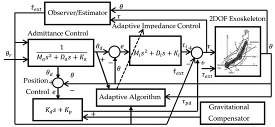
Figure 4. Hybrid adaptive impedance and position control (HAIPC): the admittance control generates desired trajectory ${\theta }_d$ based on the estimated interaction joint torque ${\widehat{\tau }}_{ext}$. The PD position control provides the trajectory tracking and the gravitational compensator makes the system transparent against gravity. The observer estimates the interaction joint torque based on the control torque $\tau$ and angular position $\theta$. Adaptive impedance control regulates and controls the interaction joint torque.

In Figure 4, the upper-limb control system is given by the following:

$$M\left(\theta \right)\ddot{\theta }+C\left(\theta ,\dot{\theta }\right)\dot{\theta }+G\left(\theta \right)=\mathsf{\tau }+{\tau }_{ext}$$

(9)

where the input control torque $\tau$ to the system is given by the following:

$$\tau ={\tau }_{pd}+{\tau }_i-{\widehat{\tau }}_{ext}$$

(10)

where ${\tau }_{pd}, {\tau }_i,$ and ${\widehat{\tau }}_{ext}$ are the admittance-based proportional derivative (PD) position control torque, adaptive impedance torque, and estimated interaction joint torque produced by human contact, respectively. Hence, after the dynamic model is obtained, the next task is to design a control law that involves position control with gravity compensation (PCGC), interaction joint torque estimation, adaptive impedance control, and stability analysis.

4.1. PCGC Design

In this work, an admittance-based PD position controller with gravitation torque compensation is used for the desired position tracking of the upper limb. Optimal values of the PD gains for proper trajectory tracking are obtained by GA optimization. The admittance control based on the estimated interaction joint torque generates a desired reference trajectory that is tracked by the position controller (GA-PD) to guide the patient’s upper limb along the desired trajectory.

$${\tau }_{pd}=K_p\left({\theta }_d-\theta \right)+K_d\frac{d}{dt}\left({\dot{\theta }}_d-\dot{\theta }\right)+{\tau }_{G\left(\theta \right)}$$

(11)

The feedforward equations for gravity compensation at the shoulder and elbow joints are given in Equations (12) and (13).

$$m_{1}g{L}_{c1}\cos \left({\theta }_1\right)+m_{2}g\left(L_1\cos \left({\theta }_1\right)+L_{c2}\cos \left({\theta }_1+{\theta }_2\right)\right)={\tau }_{sG}\left({\theta }_1,{\theta }_2\right)$$

(12)

$$m_{2}g{L}_{c2}\cos \left({\theta }_1+{\theta }_2\right)={\tau }_{eG}\left({\theta }_1,{\theta }_2\right)$$

(13)

where ${\tau }_{sG}\left({\theta }_1,{\theta }_2\right)$ and ${\tau }_{eG}\left({\theta }_1,{\theta }_2\right)$ are the gravitational torque compensators at the shoulder and elbow, respectively. With this feedforward compensation, transparency can be achieved, which makes it easier for the patient to move their limbs in a vertical direction against gravity. These gravitational compensation terms are added to the position controller, as shown in Equation (11). Furthermore, the admittance control equation is represented as follows:

$$M_a{\ddot{\theta }}_d+D_a{\dot{\theta }}_d+K_a\left({\theta }_d-{\theta }_r\right)={\tau }_{ext}$$

(14)

The desired angular position ${\theta }_d$ is given by the following:

$${\theta }_d=K_a^{-1} ({\tau }_{ext}-M_a{\ddot{\theta }}_d-D_a{\dot{\theta }}_d)+{\theta }_r$$

(15)

Thus, the gravitational compensation position controller is updated by substituting Equation (15) into Equation (11).

$${\tau }_{pd}=K_p\left(\left(K_a^{-1} \left({\tau }_{ext}-M_a{\ddot{\theta }}_d-D_a{\dot{\theta }}_d\right)+{\theta }_r\right)-\theta \right)++K_d\frac{d}{dt}\left({\dot{\theta }}_d-\dot{\theta }\right)+{\tau }_{G\left(\theta \right)}$$

(16)

Therefore, the gravitational compensation position controllers for the shoulder and elbow are given as Equations (17) and (18):

$$\begin{array}{l}{\tau }_{spd}=K_p\left(\left(K_a^{-1} \left({\tau }_{ext}-M_a{\ddot{\theta }}_d-D_a{\dot{\theta }}_d\right)+{\theta }_r\right)-{\theta }_1\right)+K_d\frac{d}{dt}\left({\dot{\theta }}_d-{\dot{\theta }}_1\right)\\ +{\tau }_{sG}\left({\theta }_1,{\theta }_2\right)\end{array}$$

(17)

$$\begin{array}{l}{\tau }_{epd}=K_p\left(\left(K_a^{-1} \left({\tau }_{ext}-M_a{\ddot{\theta }}_d-D_a{\dot{\theta }}_d\right)+{\theta }_r\right)-{\theta }_2\right)+K_d\frac{d}{dt}\left({\dot{\theta }}_d-{\dot{\theta }}_2\right)\\ +{\tau }_{eG}\left({\theta }_1,{\theta }_2\right)\end{array}$$

(18)

4.2. Interaction Joint Torque Estimation

The system has no embedded torque sensor to measure the interaction joint torque at the shoulder and elbow joints. Therefore, an extended state observer is used to estimate the unknown interaction joint torque. Generally, for a stiff contact, the equation of the environmental interaction torque at a joint is given by the following:

$$K\left({\theta }_d-{\theta }_e\right)={\tau }_{ext}$$

(19)

This implies that $K\left({\theta }_1-{\theta }_e\right)={\tau }_{ext}$ for the shoulder and $K\left({\theta }_2-{\theta }_e\right)={\tau }_{ext}$ for the elbow. Consider the joint model in Equation (7), i.e., for the shoulder, as a second-order system represented as follows:

$$\ddot{\theta }\left(t\right)={\tau }_{ext}+bu\left(t\right)$$

(20)

where ${\tau }_{ext}$ and $u\left(t\right)$ are the applied interaction joint torque and the total control joint torque. Note that for a better estimation of the interaction joint torque, the gravitational compensator is not included in the total control torque used in the observer. The state space joint angle equations are as follows:

$${\dot{\theta }}_1\left(t\right)={\theta }_2\left(t\right)$$

(21)

$${\dot{\theta }}_2\left(t\right)=\rho u\left(\theta ,t\right)+{\tau }_{ext}$$

(22)

State space equations can be extended to include the environmental interaction joint torque as a new state variable given as ${\theta }_3={\tau }_{ext}$, which yields the following:

$${\dot{\theta }}_1\left(t\right)={\theta }_2\left(t\right)$$

(23)

$${\dot{\theta }}_2\left(t\right)=\rho u\left(\theta ,t\right)+{\tau }_{ext}$$

(24)

$${\dot{\theta }}_3\left(t\right)={\dot{\tau }}_{ext}\left(\theta ,t\right)$$

(25)

Thus, the extended state observer can be designed as follows:

$${\dot{\widehat{\theta }}}_1\left(t\right)={\widehat{\theta }}_2\left(t\right)+K_1\left({\widehat{\theta }}_1\left(t\right)-{\theta }_1\left(t\right)\right)$$

(26)

$${\dot{\widehat{\theta }}}_2\left(t\right)={\widehat{\vartheta }}_3\left(t\right)+K_2\left({\widehat{\theta }}_1\left(t\right)-{\theta }_1\left(t\right)\right)+\rho u\left(\theta ,t\right)$$

(27)

$${\dot{\widehat{\theta }}}_3\left(t\right)=K_3\left({\widehat{\theta }}_1\left(t\right)-{\theta }_1\left(t\right)\right)$$

(28)

where the estimated and actual system states are ${\widehat{\theta }}_1\left(t\right),{\widehat{\theta }}_2\left(t\right),{\widehat{\theta }}_3\left(t\right)$ and ${\theta }_1\left(t\right),{\theta }_2\left(t\right),{\theta }_3\left(t\right)$, respectively. The observer gains are $K_1,K_2,K_3$ for the shoulder and $K_4,K_5,K_6$ for the elbow, and the observer error is given by $\widehat{e}\left(t\right)={\widehat{\theta }}_1\left(t\right)-{\theta }_1\left(t\right)$. The observer gains were designed for the shoulder and elbow joints separately based on the general assumption that the observer poles should be placed four to ten times to the left of the s-plane of the closed-loop poles for fast response (i.e., ${\omega }_{obs}=\left(4-10\right){\omega }_c$). Thus, in this work, ${\omega }_{obs}=6\times {\omega }_c$ is selected to calculate the gains for the shoulder and elbow joints as follows:

$K_1=3{\omega }_{obs}, K_2=3{{\omega }_{obs}}^2, K_3={{\omega }_{obs}}^3$ for shoulder joint and $K_4=3{\omega }_{obs}, K_5=3{{\omega }_{obs}}^2, K_6={{\omega }_{obs}}^3$ for elbow joint.

Therefore, the observer gain matrix is given as follows:

$$L={\left[\begin{array}{c}\begin{array}{cccc}{K}_1& K_2& K_3& 0\begin{array}{ccc}& 0& 0\end{array}\end{array}\\ \begin{array}{cccc}0& 0& 0& \begin{array}{ccc}{K}_4& K_5& K_6\end{array}\end{array}\end{array}\right]}^T$$

(29)

4.3. Adaptive Impedance Control

The dynamic model of the robot in Equations (5) and (6) with control torque and estimated interaction joint torque can be expressed as follows:

$$M\left(\theta \right)\ddot{\theta }+C\left(\theta ,\dot{\theta }\right)\dot{\theta }+G\left(\theta \right)=\mathsf{\tau }+{\tau }_{ext}$$

(30)

where $M$ is the mass and moment of inertia matrix, $C$ is the centrifugal and Coriolis torque, and $G$ is the gravitational torque. The terms $\mathsf{\tau }$ and ${\tau }_{ext}$ are the system input torque and interaction joint torque, respectively. The interaction joint torque is estimated in Section 4.2, and it will be used as the human interaction joint torque in the admittance control and adaptive impedance algorithm to update the damping and stiffness gains. A recursive least-squares algorithm (RLS) was used to tune the damping and stiffness ($D$ and $K$) constants of the impedance controller based on changes in the interaction joint torque ${\tau }_{ext}$. The adaptive algorithm was developed to update the parameters of the impedance control online based on changes in the interaction joint torque for different patients. The impedance control is shown as Equation (31).

$$M_i\left({\ddot{\theta }}_d-\ddot{\theta }\right)+D_i\left({\dot{\theta }}_d-\dot{\theta }\right)+K_i\left({\theta }_d-\theta \right)={\tau }_{ext}$$

(31)

where $M_i$, $D_i$, and $K_i$ are the inertia, damping, and stiffness coefficients of the impedance controller, respectively. In this study, the inertia $M_i$ was set at zero, and the damping and stiffness were updated based on the adaptive algorithm using the estimated interaction joint torque. Therefore, for the adaptive formulation, the impedance control is reduced to Equation (32). Since $M_i=0$ in the adaptive formulation, the impedance control reduces to Equation (32).

$$D_i\left({\dot{\theta }}_d-\dot{\theta }\right)+K_i\left({\theta }_d-\theta \right)={\tau }_{ext}$$

(32)

The human–robot interaction is assumed to be stiff; therefore, the environmental interaction joint torque is given by the following:

$${\tau }_{ext}=K_e\left({\theta }_d-{\theta }_e\right)$$

(33)

However, in this work, the environment is unknown; therefore, ${\tau }_{ext}$ is estimated using the extended state observer and is used in the adaptive algorithm to update the damping and stiffness. The interaction between the human limb and the exoskeleton changes from soft contact to stiff contact. Soft contact occurs when a human does not contribute external torque during position control. Therefore, the human limb is passive, and the exoskeleton gives the control torque to drive the joint to a certain desired position. After reaching the desired position, the patient applies an external interaction joint torque to generate muscular contraction during the exercise. In this case, referred to as the active mode, the interaction between the exoskeleton and human is stiff. The adaptive impedance controller law is as follows:

$${\tau }_{ext}=\widehat{D}\dot{e}+\widehat{K}e=\widehat{\sigma }\left(t\right){\phi }^T\left(t\right)$$

(34)

where $\widehat{\sigma }\left(t\right)=\left[\widehat{D} \widehat{K}\right]$ is the estimation vector, ${\phi }^T\left(t\right)={\left[e \dot{e}\right]}^T$ is the regression vector, $\dot{e}=\left({\dot{\theta }}_d-\dot{\theta }\right)$, and $e=\left({\theta }_d-\theta \right)$.

A cost function is defined to minimize the error between measured estimated interaction joint torque and the predictive impedance control parameters to estimate the optimal values of the stiffness and damping constants, as follows:

$$E={{\displaystyle \int }}_0^t{\left({\tau }_{ext}-{\phi }^T\left(t\right)\widehat{\sigma }\left(t\right)\right)}^{2}dt$$

(35)

Thus, the value of $E$ can be minimized by taking the derivative of Equation (35) based on the least-square method, as follows:

$$\frac{\partial E}{\partial \widehat{\sigma }\left(t\right)}=-2{{\displaystyle \int }}_0^t{\phi }^T\left(t\right)\left({\tau }_{ext}-{\phi }^T\left(t\right)\widehat{\sigma }\left(t\right)\right)dt=0$$

(36)

The adaptation process to update the stiffness and damping parameters can be achieved if $\frac{\partial E}{\partial \widehat{\sigma }\left(t\right)}=0$. Therefore, Equation (36) can be minimized to ${\tau }_{ext}={\phi }^T\left(t\right)\widehat{\sigma }\left(t\right)$ by dividing both sides of Equation (36) by $-2{{\displaystyle \int }}_0^t{\phi }^T\left(t\right)dt$. Therefore, by using the measured estimated interaction joint torque from the observer and the error and the derivative of the error from the system outputs used in ${\phi }^T\left(t\right)={\left[e \dot{e}\right]}^T$, the stiffness and damping constants would be updated. The adaptable performance can be measured based the cost function in Equation (35), and the stiffness and damping constants in the estimation vector $\widehat{\sigma }\left(t\right)$ can be estimated using the following RLS method:

$$\widehat{\sigma }\left(t\right)=\widehat{\sigma }\left(t-1\right)+J\left(t\right)\left[{\tau }_{ext}-{\phi }^T\left(t\right)\widehat{\sigma }\left(t-1\right)\right]+qp\beta \left(t\right)\left(\widehat{\sigma }\left(t-1\right)-\widehat{\sigma }\left(t-2\right)\right)$$

(37)

$$J\left(t\right)=p\beta \left(t-1\right)+\phi \left(t\right){\phi }^T\left(t\right)+q\left(1-p\right)I\phi \left(t\right)$$

(38)

$$\beta \left(t\right)=p\beta \left(t-1\right)+\phi \left(t\right){\phi }^T\left(t\right)+q\left(1-p\right)I$$

(39)

$\beta \left(t\right)$ is a covariance 2 by 2 matrix with initial value $\beta \left(0\right)={\beta }_0{I}_2$, where ${\beta }_0$ is a large positive number. Similarly, the constant terms $p$ and $q$ can be chosen such that 0 < $p$ < 1 and $q$ > 0.

The above PCGC control design was implemented for HAIPC, HIPC, and HIPCSW for a fair comparison of the three controllers, in addition to using the same method for estimating the interaction joint torque. The three controllers differed only in impedance control. Furthermore, HAIPC used adaptive impedance parameters and in-series connection without switching, whereas HIPC and HIPCSW used fixed impedance parameters. HIPC uses in-series connection without switching, and HIPCSW uses parallel connection with switching.

4.4. Stability Analysis

If the values of $M_i$, $D_i$, and $K_i$ are constant positive symmetric definite matrices, the system will be asymptotically stable. However, in this work, only $M_i$ is assumed to be constant. $D_i$ and $K_i$ are continuously updated based on the estimated interaction joint torque in the adaptive algorithm. Therefore, the stability condition is needed for time-varying stiffness and damping coefficients. The stability analysis presented is in accordance with the stability proven in [61]. From Equation (31), a new control input can be expressed as follows:

$$u={\ddot{\theta }}_d+M_i^{-1}(-D_i\left({\dot{\theta }}_d-\dot{\theta }\right)-K_i\left({\theta }_d-\theta \right)+{\tau }_{ext})$$

(40)

Thus, the input torque in Equation (30) can be expressed as follows:

$$\mathsf{\tau }=M\left(\theta \right)u+C\left(\theta ,\dot{\theta }\right)\dot{\theta }+G\left(\theta \right)-{\tau }_{ext}$$

(41)

The following Lyapunov function is considered in this work for the stability analysis of Equation (31):

$$V_1\left(\mathrm{e},\dot{e}, \mathrm{t}\right)=\frac{1}{2}{\dot{e}}^T{M}_i\left(t\right)\dot{e}+\frac{1}{2}{e}^T{K}_i\left(t\right)e$$

(42)

where $e={\theta }_d-\theta$. Taking the derivative of Equation (42) along the trajectories of Equation (31) with a constant $M_i$ and ${\tau }_{ext}=0$ yields the following equation:

$${\dot{V}}_1\left(\mathrm{e},\dot{e}, \mathrm{t}\right)={\dot{e}}^T{M}_i\left(t\right)\ddot{e}+e^T{K}_i\left(t\right)\dot{e}+\frac{1}{2}{e}^T{\dot{K}}_i\left(t\right)e$$

(43)

Based on the assumption that $M_i$ is constant and ${\tau }_{ext}=0$ from Equation (31), we obtain the following:

$$M_i\ddot{e}=-D_i\left(t\right)\dot{e}-K_i\left(t\right)e$$

(44)

Substituting Equation (44) into Equation (43) yields the following:

$${\dot{V}}_1\left(\mathrm{e},\dot{e}, \mathrm{t}\right)={\dot{e}}^T\left(-D_i\left(t\right)\dot{e}-K_i\left(t\right)e\right)+e^T{K}_i\left(t\right)\dot{e}+\frac{1}{2}{e}^T{\dot{K}}_i\left(t\right)e$$

(45)

Simplifying Equation (45) yields the following:

$${\dot{V}}_1\left(\mathrm{e},\dot{e}, \mathrm{t}\right)\le -{\dot{e}}^T{D}_i\left(t\right)\dot{e}+\frac{1}{2}{e}^T{\dot{K}}_i\left(t\right)e$$

(46)

Thus, Equation (46) is a negative semidefinite for $K_i$(t); therefore, it can be concluded that the system is stable only when the $K_i\left(t\right)$ values are either decreasing or constant starting from the origin. This is because if $K_i\left(t\right)$ increases with time, the system will become unstable.

5. Results and Discussion

This section presents the simulation setup and the results. Two different therapy exercises are conducted. The first exercise is isotonic exercise, which helps provide the patient with the most useful muscular contraction improvements for regular joint function. The second exercise is active assistive exercise, which helps the patient to build up strength in their limbs. In all cases, the results of the proposed HAIPC are discussed, and its performance is compared with those of HIPC and HIPCSW.

5.1. Setup

This section presents the simulation setup of HAIPC, HIPC, and HIPCSW. The performance of the proposed HAIPC was compared with those of HIPCSW [15] and HIPC [35] to evaluate the effectiveness of the proposed control. The desired interaction joint torque is represented in Equation (47), which represents the physical human–robot interaction joint torque at the shoulder and elbow joints. In real time, the magnitude of the interaction joint torque is unknown; therefore, in this work, its values are estimated using ESO along the joint angular position. However, for simulation purposes, a known human interaction joint torque is used, as given in Equation (47). The magnitude of the interaction joint torque differs from patient to patient depending on the level of recovery and frequency of therapy. In these simulations, two desired interaction joint torques applied by the patients at different time intervals with magnitudes of 3 and 2.25 Nm are considered. Herein, the human–robot interaction is of two modes: passive mode, assuming no interaction force (zero torque) applied from the human; and active mode, where different magnitudes of torque are applied.

$${\mathit{\tau }}_{\mathit{e}\mathit{x}\mathit{t}}=\left\{\begin{array}{ccc}\mathbf{0.0} \mathbf{N}\mathbf{m}& \mathbf{0}\le \mathbf{t}<\mathbf{7}& \mathbf{Passive\; Mode}\\ \mathbf{3.0} \mathbf{N}\mathbf{m}& \mathbf{7}\le \mathbf{t}<\mathbf{9}& \mathbf{Active\; Mode}\\ \mathbf{0.0} \mathbf{N}\mathbf{m}& \mathbf{9}\le \mathbf{t}<\mathbf{14}& \mathbf{Passive\; Mode}\\ \mathbf{2.25} \mathbf{N}\mathbf{m}& \mathbf{14}\le \mathbf{t}<\mathbf{16}& \mathbf{Active\; Mode}\\ \mathbf{0.0} \mathbf{N}\mathbf{m}& \mathbf{16}\le \mathbf{t}<\mathbf{20}& \mathbf{Passive\; Mode}\end{array}\right.$$

(47)

The passive mode runs when the patient’s limbs are completely driven by the exoskeleton’s motors during physical therapy along the desired angular trajectories. In this case, the input control torque is closer to admittance position control because there is soft contact between the exoskeleton and human limbs. The adaptive impedance control torque is almost zero during soft contact. On the other hand, the active mode is when the patient can apply some torque during therapy to strengthen their arms or for muscular contraction. In this study, the robot first moves the human upper limb to a certain position within the limits of the joint movements. The patient will then be asked to apply some torque to move their joints. Based on Equation (47), the patient performs an exercise by applying torque to move their limbs together while the exoskeleton applies weight in the up–down direction, thereby switching from passive mode to active mode.

5.2. Simulation Results

The simulation was conducted using MATLAB/Simulink 2019a with a fixed step size of 0.001 s. The same GA_PD gains for motor 1 and motor 2 were used for HAIPC, HIPC and HIPCSW in the simulation with values of $K_p=600$, $K_d=100$ and $K_p=570$, $K_d=70, \mathrm{respectively}$. Similarly, the admittance control gains used were $M_a=1$, $D_a=2\sqrt{M_a{K}_a}$, and $K_a=10$ for the HAIPC, HIPC, and HIPCSW. In addition, the impedance control gains for HIPC and HIPCSW were $M_i=0$, $D_i=2\times 0.7\times \sqrt{K_i}$, and $K_i=200$. Also, $M_i=0$ for HAIPC and $D_i$ and $K_i$ are updated online based on active mode interaction joint torque.

5.2.1. Case I: Isotonic Exercise

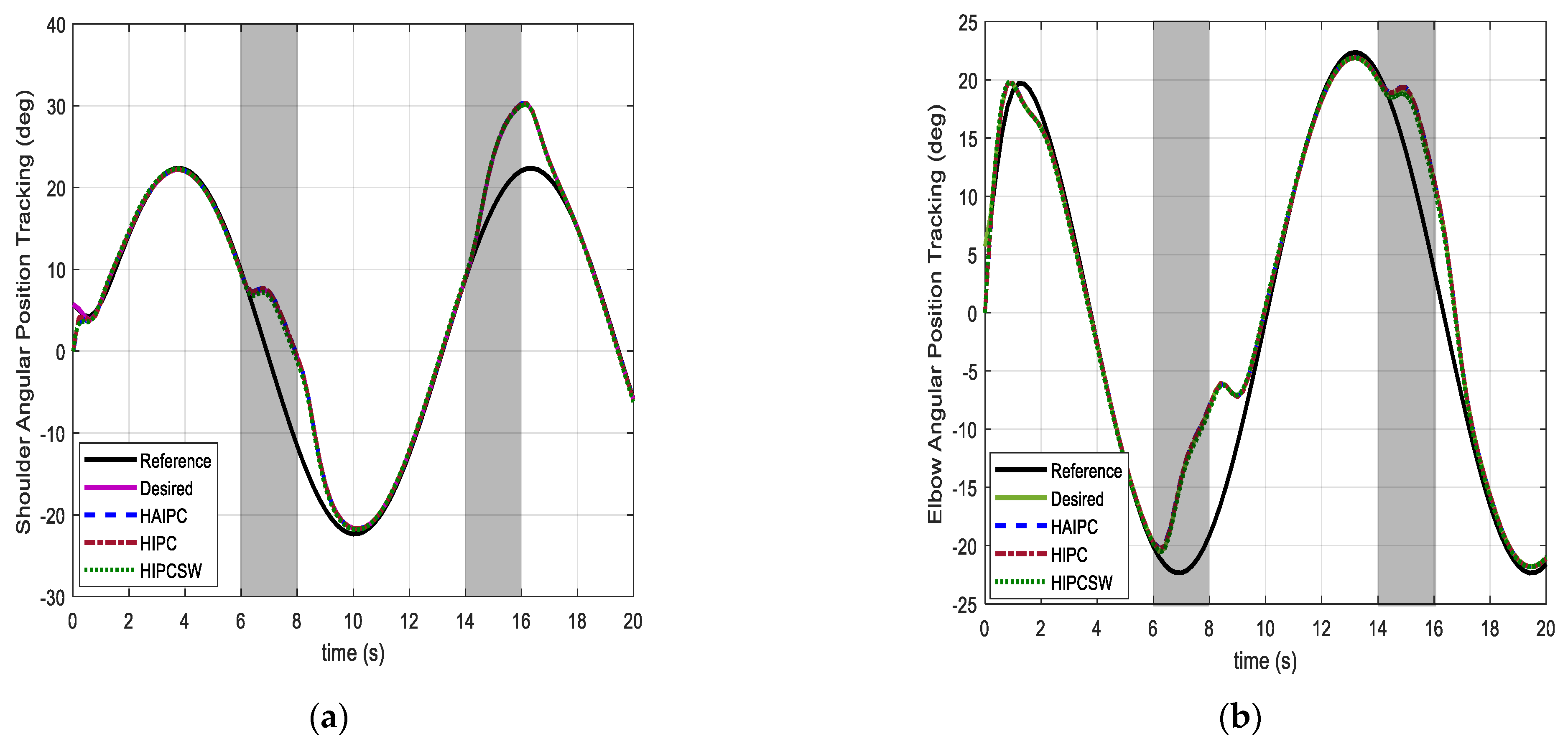
In this exercise, the robot will first move the patient’s limb to a certain desired position in the passive mode, i.e., position control. Then, the patient will be asked to apply an interaction joint torque, as described in Equation (47), to move their limbs together with the exoskeleton weight. The addition of feedforward gravity compensation makes the human exoskeleton transparent against gravity at the equilibrium position. The transparency of the system makes it easier for the patient to move their hand upward during the active mode without having to counter the gravitational torque. In this case, the patient initiates the active muscular contraction exercise independently to recover joint functionality. During this exercise, the patient switches from the passive mode to the active mode. In the active mode, the patient will lift their limb together with the exoskeleton upward from the equilibrium position for a few seconds and then return to the same position by switching from the active mode to the passive mode. Figure 5a,b shows the desired step angular position tracking for the shoulder and elbow joints, respectively. From these figures, it can be observed that, at first, the shoulder joint moves from 0° to 31.51° (0.55 rad) and the elbow joint from 0° to 42.97° (0.75 rad). After 7 s, the patient switches to the active mode and lifts their limb together with the exoskeleton upward for 2 s, as seen in the shaded area (i.e., 7–9 s), and then returns to the equilibrium position, thereby switching back to the passive mode at 11 s. After some rest, the patient repeats the process again from 14 s to 16 s. In real time, the applied interaction joint torque during the active mode is unknown and needs to be measured. However, in the simulation, the known human desired interaction joint torque in Equation (47) was applied, and an ESO was used to estimate the interaction joint torque.

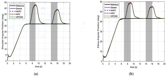
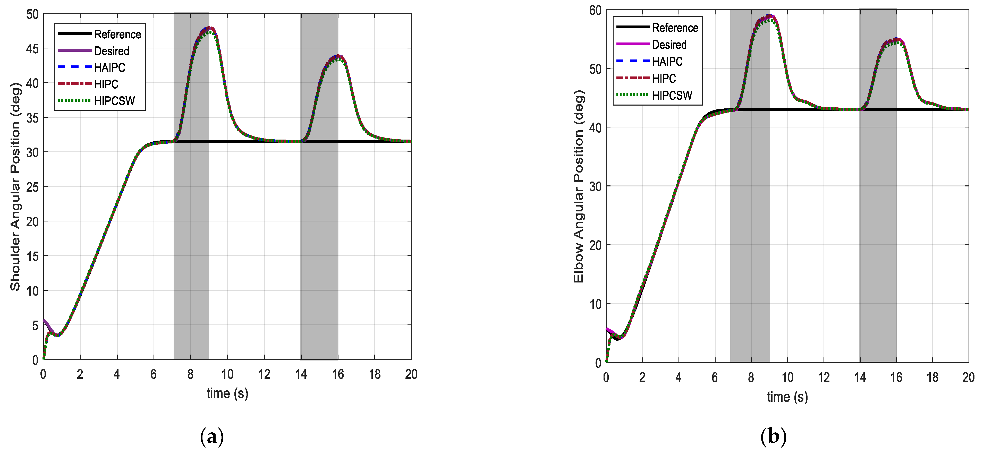
Figure 5. Angular positions of (a) shoulder and (b) elbow.

Healthy people can move their shoulder and elbow joints to around 135 degrees. For patients at the first stage of rehabilitation, we choose reference angular positions to be between 0 to 60 degrees. The desired angular position is generated when a contact interaction joint torque is applied. The admittance controller based on the interaction joint torque for compliance generates a new trajectory (desired). Thus, the reference is the trajectory position when there is no interaction joint torque between the human and exoskeleton (i.e., in passive mode), and when there is interaction joint torque, a desire trajectory is generated for compliance (i.e., in active mode). Both reference and desired trajectories are to be tracked by the patient’ joints under passive and active modes, respectively.

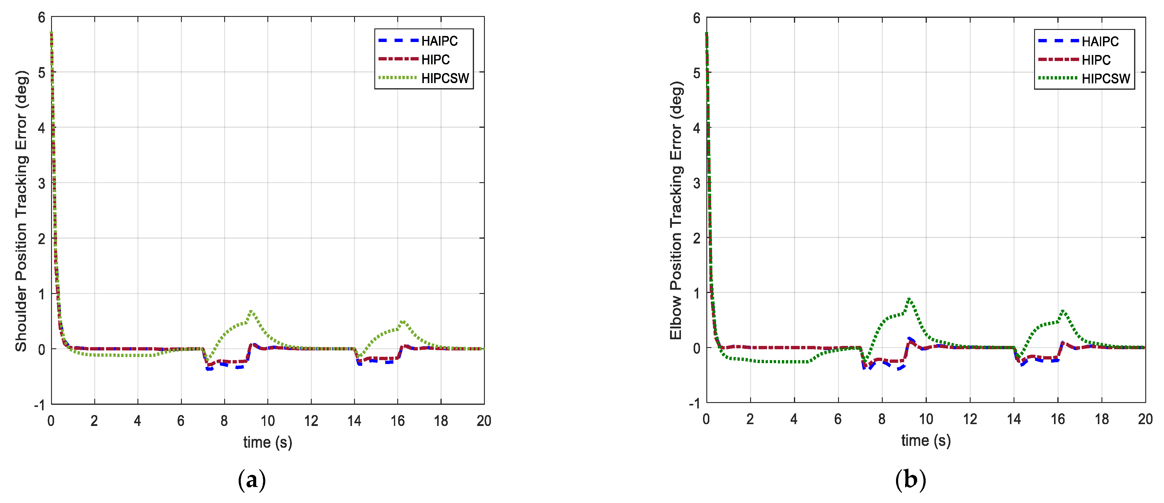
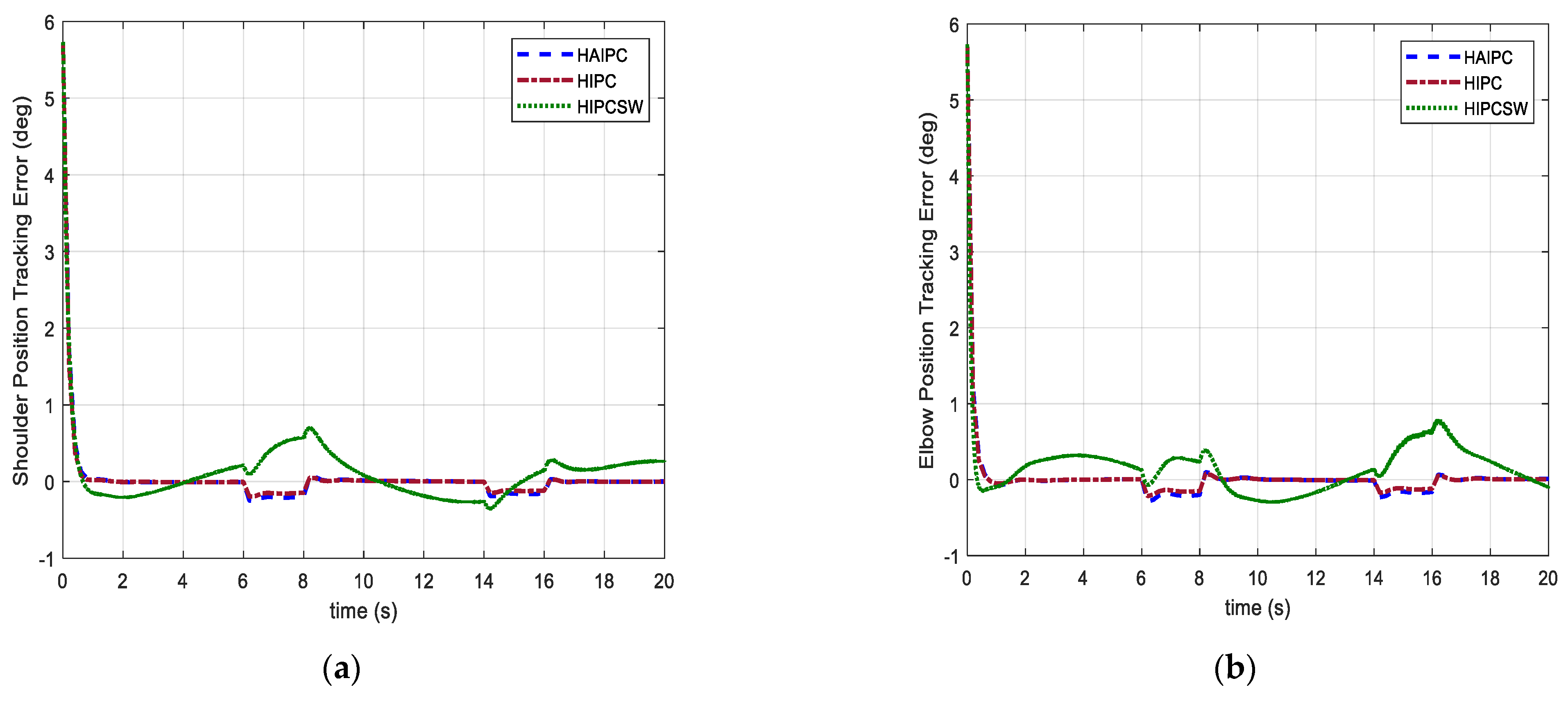
It can be observed from Figure 5a,b that the controllers have good position tracking performance. The black line represents the reference angular position input ${\theta }_r$, which is used by the admittance controller to generate the desired angular position ${\theta }_d$ based on the estimated interaction torque. The desired angular trajectory ${\theta }_d$ is tracked by the HAIPC, HIPC, and HIPCSW controllers. The position tracking error of the three controllers is shown in Figure 6a,b. The mean absolute error (MAE) was used as a tracking performance index in this study. In addition, for this discussion, the MAE values were rounded up to two decimal places; however, the actual values are given in Table 3. The MAE values in degrees for HAIPC, HIPC, and HIPCSW for the shoulder and elbow positions were measured and recorded as 0.14° and 0.13° for HAIPC, 0.12° and 0.11° for HIPC, and 0.20° and 0.26° for HIPCSW. From the results, HIPC performed slightly better than HAIPC in accurate tracking, but both HIPC and HAIPC performed much better than HIPCSW. Based on the results, the HIPC provides better position tracking than the proposed HAIPC and HIPCSW. Nevertheless, in all cases, the tracking errors produced by all three controllers are not significant and might not result in injury or discomfort to the patient.

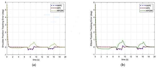
Figure 6. Angular position errors of (a) shoulder and (b) elbow.

Table 3. Case I results summary.

Control Method	Position Tracking MAE (Degree)		Torque Tracking MAE (Nm)		Control Torque MAV (Nm)
	Shoulder	Elbow	Shoulder	Elbow	Shoulder	Elbow
HAIPC	0.1412	0.1388	0.2345	0.2783	1.2685	1.2112
HIPC	0.1232	0.1198	0.2352	0.2801	1.4692	1.4093
HIPCSW	0.2045	0.2610	0.2348	0.2755	8.1502	13.6272

MAE: mean absolute error; MAV: mean absolute value.

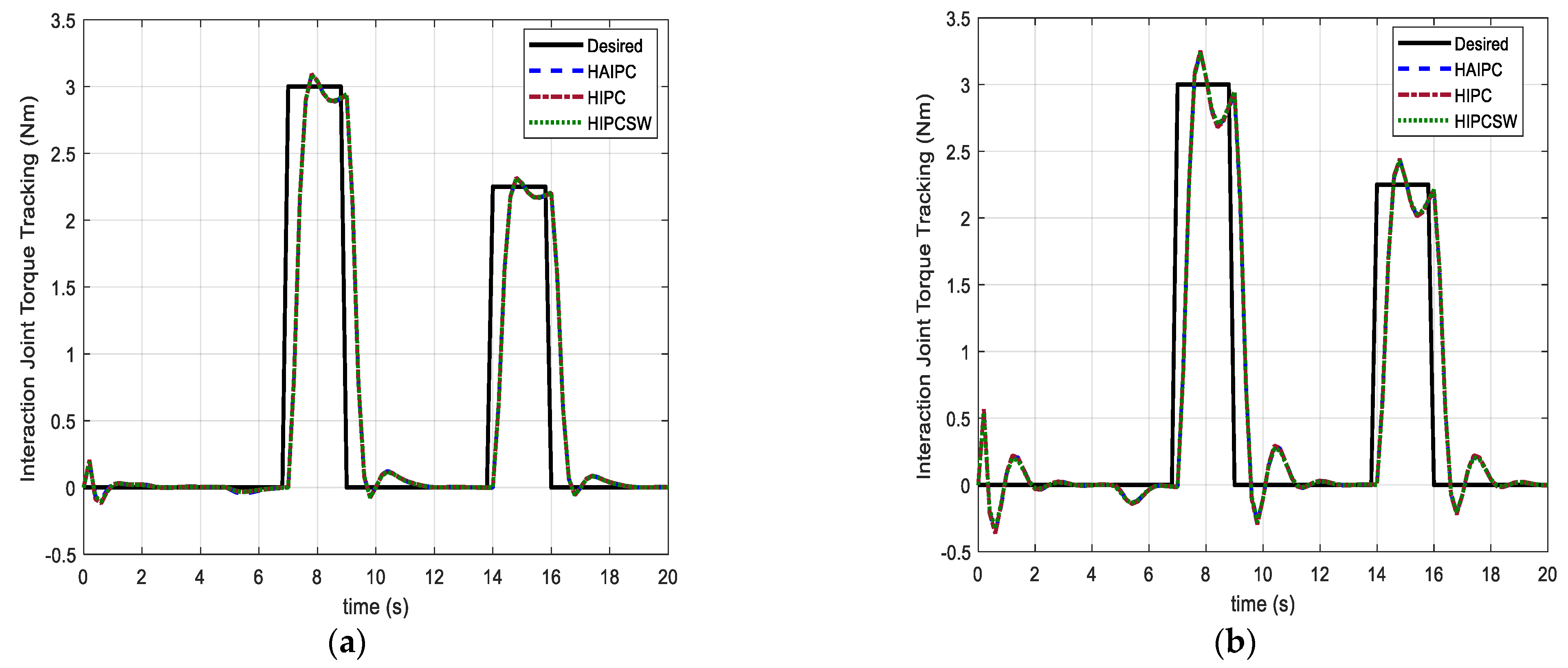
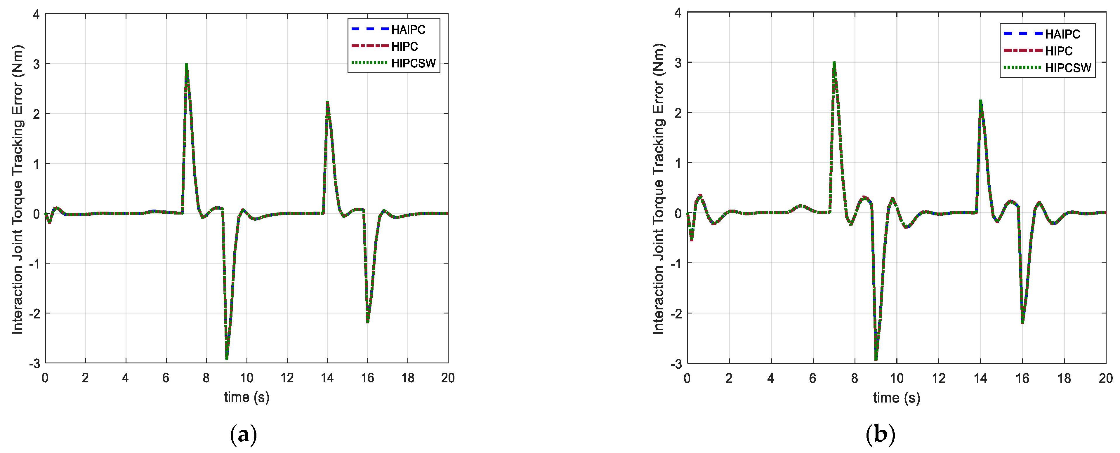
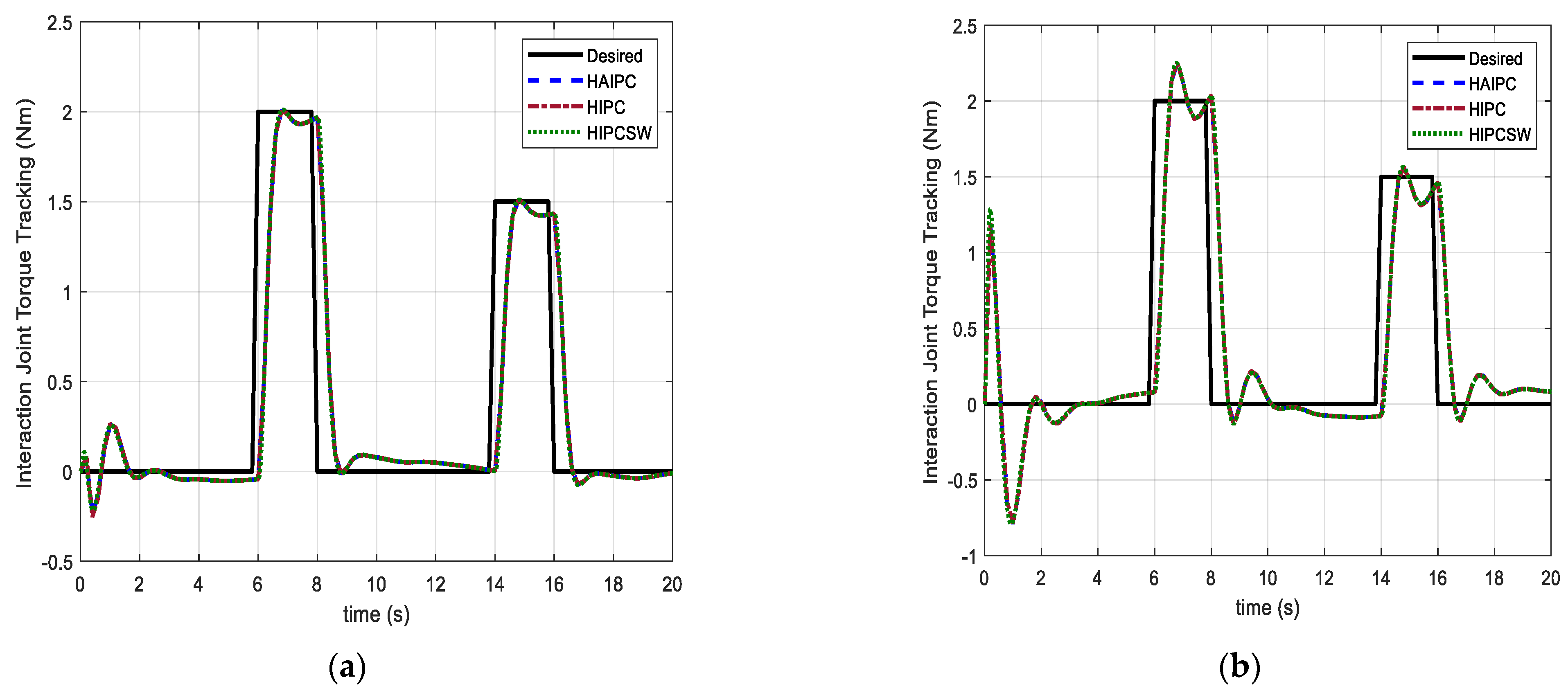
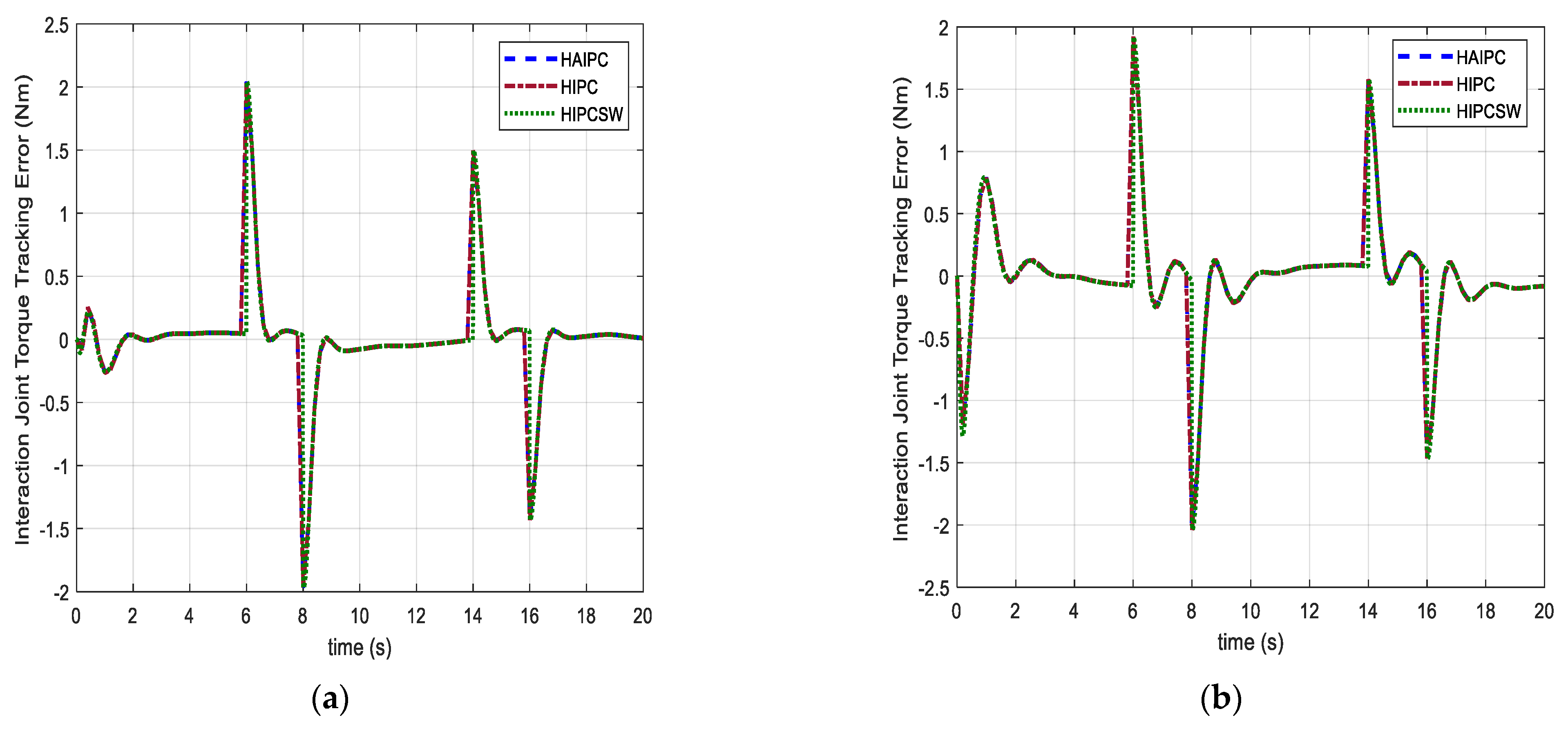
Similarly, the performance of the three controllers was measured on the basis of the desired interaction joint torque tracking, which was estimated using ESO. Initially, during the active mode, a desired interaction joint torque of 3 Nm was applied by the patient to move the joints to approximately 15.5°. In the second attempt, the joints were moved from the equilibrium position to about 12.05° with 2.25 Nm. Figure 7a,b shows the desired human interaction joint torque tracking. It was found that HIPCSW has the lowest tracking error compared to HAIPC and HIPC. The interaction joint torque tracking error is shown in Figure 8a,b. The MAE values obtained for the interaction joint torque of the shoulder and elbow joints are 0.23 Nm and 0.28 Nm for HAIPC, 0.23 Nm and 0.28 Nm for HIPC, and 0.23 Nm and 0.27 Nm for HIPCSW, respectively. From the obtained results, all the methods produce good torque tracking performance for the desired interaction joint torque. The intermediate results of the estimator occur at the points of interactions (i.e., at 6 s and 14 s), which show some transient behavior with overshoot. This occurs due to the fast tracking effort of the estimator which was based on the selection of ${\omega }_{obs}=6\times {\omega }_c$. If a smaller value of the observer frequency was used (i.e., ${\omega }_{obs}=4\ast {\omega }_c$), there would be less overshoot but with a slow estimation response.

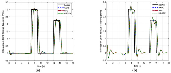
Figure 7. Interaction joint torques of (a) shoulder and (b) elbow.

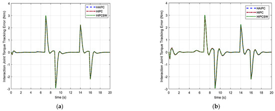
Figure 8. Interaction joint torque errors of (a) shoulder and (b) elbow.

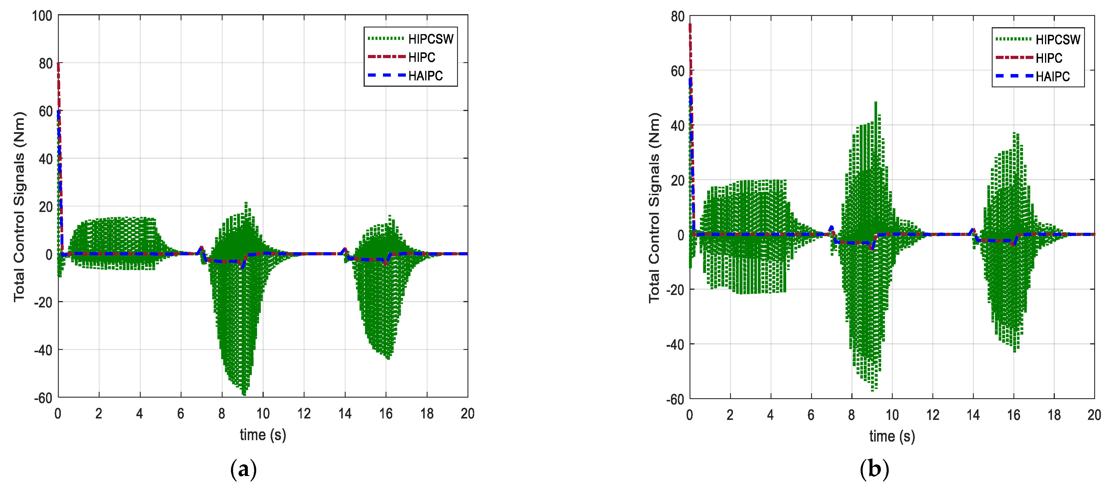
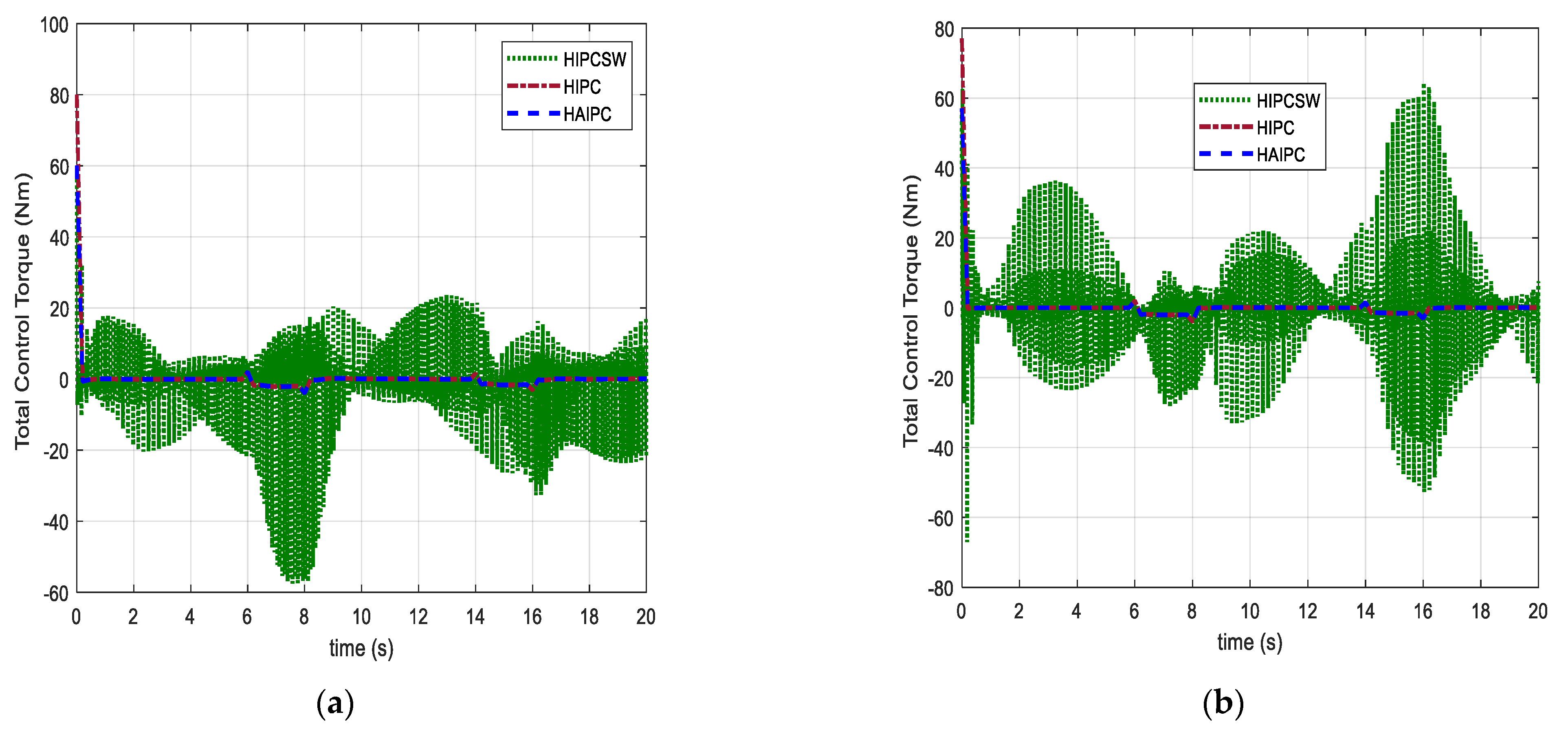
Furthermore, the performance of the proposed HAIPC as compared to HIPC and HIPCSW was assessed on the basis of the mean absolute value (MAV) of the control input torque. Figure 9a,b shows the control input torque of the three controllers without the gravitational compensator. For similar performance in position and torque tracking, it can be observed that the HIPC and HIPCSW have the highest MAV. In addition, the HIPCSW shows a chattering effect, which is a result of high-frequency switching between the two controllers. The MAVs of the HAIPC were 1.26 Nm and 1.21 Nm for the shoulder and elbow joints, respectively. Similarly, the MAVs of the HIPC and HIPCSW controllers were 1.47 Nm and 1.41 Nm and 8.15 Nm and 13.63 Nm for the shoulder and elbow joints, respectively. The MAVs show that the proposed HAIPC has less control torque consumption compared to HIPC and HIPCSW. The percentage reductions in MAV for shoulder and elbow joints compared with HIPC were 13.7% and 14%, respectively. Similarly, high percentage reductions in MAV were observed as compared to HIPCSW by 84% and 91%, respectively. The highest percentage reduction in MAV recorded compared with HIPCSW was because of signal chattering resulting from the high switching frequencies, as observed in Figure 9a,b. This is a disadvantage of the method, as aforementioned in the Introduction section. The superiority of the proposed control was found based on the control input torque consumption. The HAIPC has the smallest MAV for control input torque to produce similar desired performance results compared to HIPC and HIPCSW.

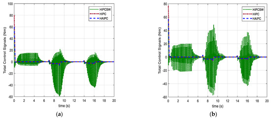
Figure 9. Total control torques for (a) shoulder and (b) elbow.

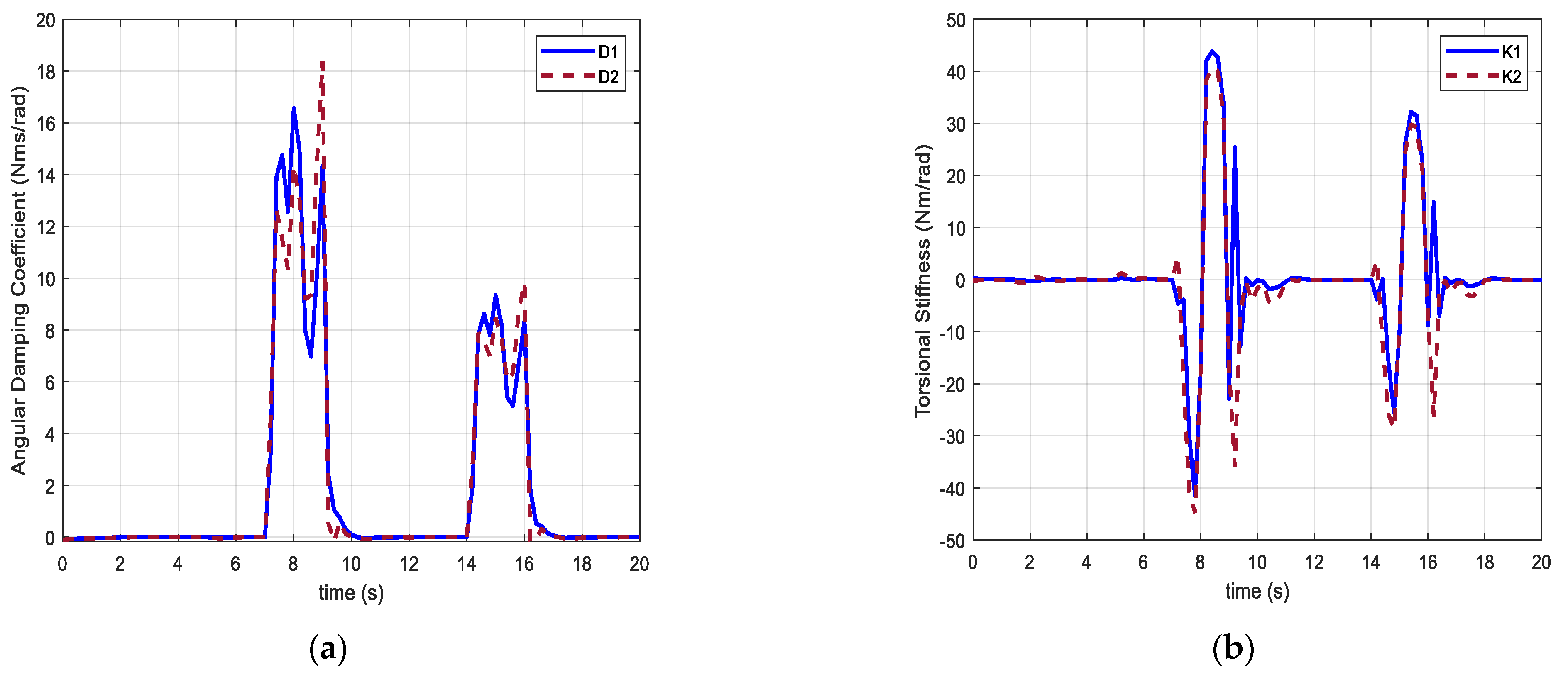
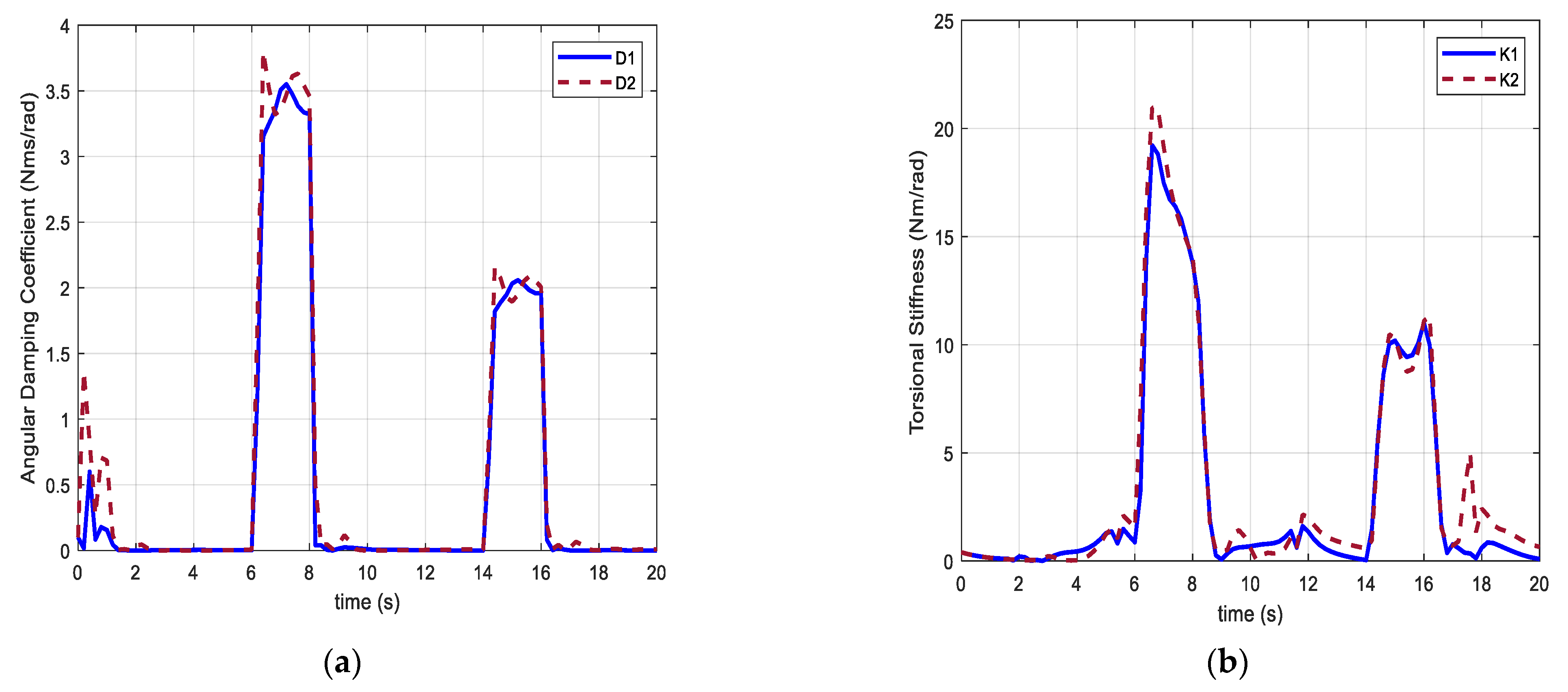
Figure 10a,b shows the values of the adaptive parameters, which are only high when an external torque is applied by the human, and they reduce to small values close to zero when the human interaction joint torque is zero. This shows that the adaptive impedance control only contributes significant torque during the active mode and reduces torque to small values during the passive mode. Thus, the proposed HAIPC approach does not require switching because it yields similar positions and torque tracking results as those obtained using HIPCSW. In addition, the chattering effect has been avoided, which might seriously affect the patient or cause discomfort, as the patient wearing the exoskeleton will feel the vibrations. A summary of the results obtained from Case I is given in Table 3.

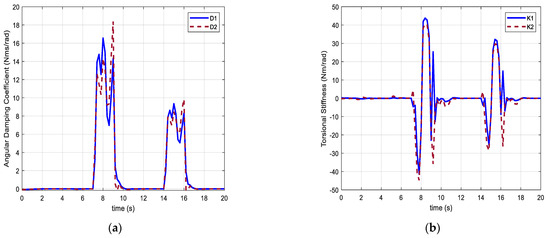
Figure 10. Adaptive parameters (a) estimated damping and (b) estimated stiffness.

5.2.2. Case II: Active-Assistive Exercise

The aim of this exercise is to allow the patient to strengthen their limb during therapy. During this exercise, the physiotherapist continuously moves the patient’s upper limb up and down in a sinusoidal manner for a fixed time. In the process, the physiotherapist asks the patient to apply some effort that sometimes deviates from the actual desired trajectory guided by the physiotherapist. At this time, the mode changes from passive to active. During this exercise, the physiotherapist does not resist the applied effort of the patient (compliance). The same idea is employed in this work with the wearable exoskeleton. First, the exoskeleton is in control of the patient’s limb (passive mode) in tracking a predefined trajectory. After some time, the patient applies some interaction joint torque at both the shoulder and elbow joints to strengthen their joints. In this study, for this exercise, the patient applied 2 Nm at 6 s to switch from passive mode to active mode and then returned to the passive mode at 10 s. Again, after some time under passive mode therapy, the patient applied 1.5 Nm to strengthen their arm again at 14 s. Figure 11a,b shows the sinusoidal trajectory reference tracking and exoskeleton compliance, as seen in the shaded area from 6 s to 8 s, and the same has been shown from 14 s to 16 s due to human interaction joint torque.

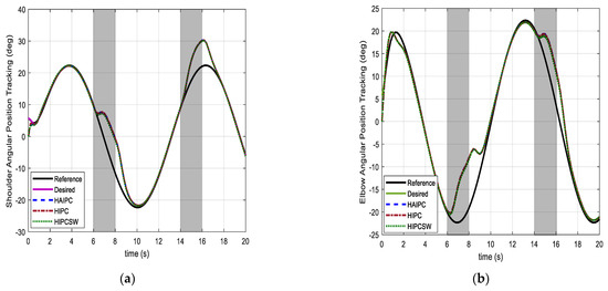
Figure 11. Angular positions of (a) shoulder and (b) elbow.

It can be deduced from Figure 11a,b that all three controllers performed excellently in tracking the sinusoidal position trajectory with good compliance to the human-applied external torque. However, to measure individual performance, MAE was used to calculate the trajectory tracking error. The MAE values for shoulder and elbow were 0.12° and 0.12° for HAIPC, 0.11° and 0.11° for HIPC, and 0.28° and 0.30° for HIPCSW, respectively. The MAE values indicate that HIPC has the lowest position tracking error for both shoulder and elbow joints, whereas HIPCSW has the highest MAE values. These can be clearly seen in Figure 12a,b. The interaction joint torque tracking control is shown in Figure 13a,b. A good tracking performance was recorded for all three controllers. The calculated MAE values of torque tracking error from Figure 14a,b are 0.18 Nm and 0.24 Nm for HAIPC, 0.18 Nm and 0.24 Nm for HIPC, and 0.18 Nm and 0.24 Nm for HIPCSW. The results show that the controllers had similar performances in torque tracking with approximately the same MAE for torque tracking error. However, HIPC provides the best results in position tracking compared to HAIPC and HIPCSW.

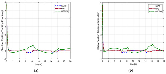
Figure 12. Angular position errors of (a) shoulder and (b) elbow.

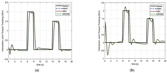
Figure 13. Interaction joint torques of (a) shoulder and (b) elbow.

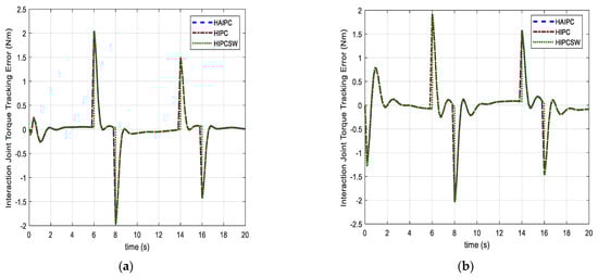
Figure 14. Interaction joint torque errors of (a) shoulder and (b) elbow.

The main advantage of the proposed HAIPC control is that it consumes less control input torque, as shown in Figure 15a,b. The MAVs of the control input torques obtained using the data from Figure 15a,b were found to be 1.06 Nm and 1.01 Nm for HAIPC, 1.26 Nm and 1.20 Nm for HIPC, and 13.35 Nm and 23.48 Nm for HIPCSW. From the MAV, the proposed HAIPC reduced the control torque by 15.6% and 17% compared with HIPC for the shoulder and elbow joints, respectively. Similarly, HAIPC reduced the shoulder and elbow control input torque by 92% and 96%, respectively, compared with HIPCSW. These results show that the proposed method HAIPC is suitable for less control torque consumption. The highest percentage reductions found in comparison with HIPCSW result from the high-frequency chattering effect, resulting from the switching mechanism in HIPCSW. Figure 16a,b shows the adaptive parameters used to update the adaptive impedance controller based on the estimated human interaction joint torque measured by the ESO. It was observed that the values of the stiffness and damping increased at the points of contact (i.e., active mode), which were at 6 and 14 s of the simulation time. The parameters reduced to almost zero when there was no interaction torque, i.e., during the passive mode. A summary of the results obtained from Case II is given in Table 4 and the list of all symbols is provided in Table 5.

Figure 15. Total control torques of (a) shoulder and (b) elbow.

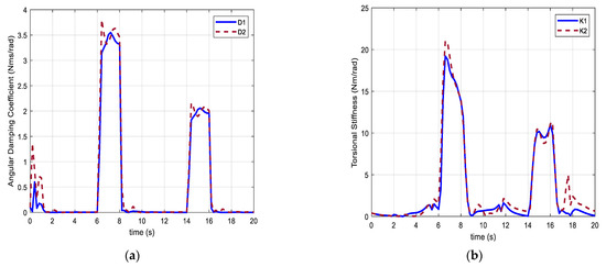
Figure 16. Adaptive parameters (a) estimated damping and (b) estimated stiffness.

Table 4. Case II results summary.

Control Method	Position Tracking MAE (Degree)		Torque Tracking MAE (Nm)		Control Torque MAV (Nm)
	Shoulder	Elbow	Shoulder	Elbow	Shoulder	Elbow
HAIPC	0.1258	0.1212	0.1829	0.2409	1.0625	1.0025
HIPC	0.1101	0.1075	0.1836	0.2413	1.2604	1.2000
HIPCSW	0.2784	0.2996	0.1820	0.2407	13.3488	23.4849

MAE: mean absolute error; MAV: mean absolute value.

Table 5. List of symbols of variables.

Parameters	Symbols
Centre of mass of link 1	$CM1$
Centre of mass of link 2	$CM2$
Inertia matrix	$M\left(\theta \right)$
Centrifugal and Coriolis torque	$C\left(\theta ,\dot{\theta }\right)$
Gravitational torque	$G\left(\theta \right)$
External torque	${\tau }_{ext}$
Shoulder control torque	${\tau }_s$
Elbow control torque	${\tau }_e$
Proportional derivative (PD) position control torque	${\tau }_{pd}$
Impedance torque	${\tau }_i$
Estimated interaction joint torque	${\widehat{\tau }}_{ext}$
Shoulder joint observer gains	$K_1,K_2,K_3$
Elbow joint observer gains	$K_4,K_5,K_6$
Observer frequency	${\omega }_{obs}$
Inertia constant of the impedance control	$M_i$
Damping constant of the impedance control	$D_i$
Stiffness constant of the impedance control	$K_i$
Inertia constant of the admittance control	$M_a$
Damping constant of the admittance control	$D_a$
Stiffness constant of the admittance control	$K_a$
Proportional gain of the PD controller	$K_p$
Derivative gain of the PD controller	$K_d$
Estimation vector	$\widehat{\sigma }\left(t\right)$
Regression vector	${\phi }^T\left(t\right)$
Covariance matrix	$\beta \left(t\right)$
Proportional derivative	PD
Genetic algorithm proportional derivative	GA_PD
Extended state observer	ESO
Recursive least-squares	RLS
Hybrid adaptive impedance position control	HAIPC
Hybrid impedance position control	HIPC
Hybrid impedance position control with switch	HIPCSW
Mean absolute error	MAE
Mean absolute value	MAV

6. Conclusions

A hybrid adaptive impedance control (HAIPC) was proposed and implemented successfully on a wearable upper limb rehabilitation robot model in MATLAB. The proposed method uses the estimated interaction joint torque to update the parameters of the adaptive impedance controller. The performance of the proposed HAIPC was measured based on the MAE of position tracking and torque tracking and the MAV of the control input torque. The implementation was conducted based on two different exercises (i.e., Case I: isotonic exercise and Case II: active assistive exercise), and it was found that in both cases, the proposed HAIPC control outperformed the HIPC and HIPCSW in minimizing the control input torque. However, it was found that the HIPC performed better in minimizing the position tracking error as compared to the HAIPC and HIPCSW, with lower MAE values for both shoulder and elbow angular positions. The MAE values measured in degrees for shoulder and elbow positions under Case I were found to be 0.14° and 0.13°, 0.12° and 0.11°, and 0.20° and 0.26° for HAIPC, HIPC, and HIPCSW, respectively. Similarly, the HIPCSW exhibits slightly better torque tracking performance with the smallest MAE of torque tracking compared to HAIPC and HIPC. The MAE values for the shoulder and elbow were obtained as 0.23 Nm and 0.28 Nm for HAIPC, 0.23 Nm and 0.28 Nm for HIPC, and 0.23 Nm and 0.27 Nm for HIPCSW, respectively. The proposed method can be applied to other forms of rehabilitation exoskeletons. The main advantage of the proposed method was found in its ability to minimize the control input torque. The percentage reductions in MAV for shoulder and elbow joints compared with HIPC were 13.7% and 14%, and, as compared to HIPCSW, the proposed method reduced the control input torques by 84% and 91%. Similar results were obtained in Case II where the MAE values for shoulder and elbow trajectory tracking were obtained as 0.12° and 0.12° for HAIPC, 0.11° and 0.11° for HIPC, and 0.28° and 0.30° for HIPCSW, respectively. Also, the MAV of the control input torques obtained were found to be 1.06 Nm and 1.01 Nm for HAIPC, 1.26 Nm and 1.20 Nm for HIPC, and 13.35 Nm and 23.48 Nm for HIPCSW. This shows that the proposed HAIPC reduced the control torques for the shoulder and elbow joints by 15.6% and 17% and by 92% and 96%, as compared with HIPC and HAIPC, respectively. Furthermore, the proposed method has the combined advantages of both HIPC and HIPCSW, namely less control torque (i.e., current consumption), no chattering in the control signal, and less starting torque. In addition, an extended state observer was used for interaction joint torque estimation, which eliminated the need for a torque sensor. The disadvantage of this method was based on the complexity of the adaptive algorithm; however, it has good parameter estimation.

For practical implementation, the fine tuning of the control gains is required to compensate for the discrepancy between the real system and its mathematical model. Appropriate filters must be applied to reduce noise from sensor data for accurate estimation. The proposed control in this work was implemented on a 2DOF upper limb exoskeleton model via simulation. However, it can be extended and implemented both in simulation and in physical prototypes of higher DOF upper limb (i.e., shoulder, elbow, and wrist joints) and lower limb (i.e., hip, knee, and ankle joints) exoskeletons. Therefore, in our future work, a shoulder–elbow–wrist upper limb exoskeleton will be designed and fabricated for experimental studies of the proposed HAIPC. Torque sensors will be applied to validate the estimation of the interaction joint torque using this proposed extended state observer. Furthermore, the RLS algorithm used for the parameter adaptation of the impedance control parameters in this work usually comes with complexity and computational cost. Other simple algorithms such as least mean squares, recursive regularized least-squares, and stochastic gradient descent algorithms could be considered for future improvement.

References

- Tantagunninat, T.; Wongkaewcharoen, N.; Pornpipatsakul, K.; Chuengpichanwanich, R.; Chaichaowarat, R. Modulation of joint stiffness for controlling the cartesian stiffness of a 2-DOF planar robotic arm for rehabilitation. In Proceedings of the 2023 IEEE/ASME International Conference on Advanced Intelligent Mechatronics, Seattle, WA, USA, 28–30 June 2023; pp. 598–603. [Google Scholar]
- Mesatien, T.; Suksawasdi, R.; Ayuthaya, N.; Chenviteesook, A.; Chaichaowarat, R. Position accuracy of a 6-DOF passive robotic arm for ultrasonography training. In Proceedings of the IEEE Region 10 Technical Conference, Chiang Mai, Thailand, 31 October–3 November 2023; pp. 841–846. [Google Scholar]
- Chaichaowarat, R.; Prakthong, S.; Thitipankul, S. Transformable wheelchair–exoskeleton hybrid robot for assisting human locomotion. Robotics 2023, 12, 16. [Google Scholar] [CrossRef]
- Chaichaowarat, R.; Macha, V.; Wannasuphoprasit, W. Passive knee exoskeleton using brake torque to assist stair ascent. In Proceedings of the IEEE Region 10 Technical Conference, Osaka, Japan, 16–19 November 2020; pp. 1165–1170. [Google Scholar]
- Chaichaowarat, R.; Nishimura, S.; Nozaki, T.; Krebs, H.I. Work in the time of COVID-19: Actuators and sensors for rehabilitation robotics. IEEJ J. Ind. Appl. 2021, 11, 256–265. [Google Scholar] [CrossRef]
- Chaichaowarat, R.; Nishimura, S.; Krebs, H.I. Design and modeling of a variable-stiffness spring mechanism for impedance modulation in physical human–robot interaction. In Proceedings of the 2021 IEEE International Conference on Robotics and Automation, Xi’an, China, 30 May–5 June 2021; pp. 7052–7057. [Google Scholar]
- Ullah, Z.; Chaichaowarat, R.; Wannasuphoprasit, W. Variable damping actuator using an electromagnetic brake for impedance modulation in physical human–robot interaction. Robotics 2023, 12, 80. [Google Scholar] [CrossRef]
- Hogan, N. Impedance Control: An Approach to Manipulation. In Proceedings of the American Control Conference, San Diego, CA, USA, 6–8 June 1984; pp. 304–313. [Google Scholar] [CrossRef]
- Hogan, N. The mechanics of multi-joint posture and movement control. Biol. Cybern. 1985, 52, 315–331. [Google Scholar] [CrossRef] [PubMed]
- Alexandre, R.; Emelie, S.; Marc, D. Enhancing Human Mobility Exoskeleton Comfort Using Admittance Controller. WSEAS Trans. Biol. Biomed. 2021, 18, 24–31. [Google Scholar] [CrossRef]
- Nyulangone Health. Available online: https://nyulangone.org/news/computer-tool-can-track-stroke-rehabilitation-boost-recovery (accessed on 17 February 2024).
- Arents, J.; Abolins, V.; Judvaitis, J.; Vismanis, O.; Oraby, A.; Ozols, K. Human–Robot Collaboration Trends and Safety Aspects: A Systematic Review. J. Sens. Actuator Netw. 2021, 10, 48. [Google Scholar] [CrossRef]
- Chiou, S.J.; Chu, H.R.; Li, I.H.; Lee, L.W. A Novel Wearable Upper-Limb Rehabilitation Assistance Exoskeleton System Driven by Fluidic Muscle Actuators. Electronics 2023, 12, 196. [Google Scholar] [CrossRef]
- Anderson, R.; Spong, M.W. Hybrid impedance control of robotic manipulators. IEEE J. Robot. Autom. 1988, 4, 549–556. [Google Scholar] [CrossRef]
- Ott, C.; Mukherjee, R.; Nakamura, Y.A. Hybrid System Framework for Unified Impedance and Admittance Control. J. Intell. Robot. Syst. 2015, 78, 359–375. [Google Scholar] [CrossRef]
- Liu, G.J.; Goldenberg, A.A. Robust hybrid impedance control of robot manipulators. In Proceedings of the 1991 IEEE International Conference on Robotics and Automation, Sacramento, CA, USA, 9–11 April 1991; pp. 287–292. [Google Scholar]
- Akdoaän, E.; Aktan, M.E.; Koru, A.T.; Arslan, M.S.; Atlıhan, M.; Kuran, B. Hybrid impedance control of a robot manipulator for wrist and forearm rehabilitation: Performance analysis and clinical results. Mechatronics 2018, 49, 77–91. [Google Scholar] [CrossRef]
- Kim, Y. Hybrid-Mode Impedance Control for Position/Force Tracking in Motor-System Rehabilitation. Int. J. Adv. Robot. Syst. 2015, 12, 79. [Google Scholar] [CrossRef]
- Ye, D.; Yang, C.; Jiang, Y.; Zhang, H. Hybrid impedance and admittance control for optimal robot–environment interaction. Robotica 2024, 42, 510–535. [Google Scholar] [CrossRef]
- Formenti, A.; Bucca, G.; Shahid, A.A.; Piga, D.; Roveda, L. Improved impedance/admittance switching controller for the interaction with a variable stiffness environment. Complex Eng. Syst. 2022, 2, 12. [Google Scholar] [CrossRef]
- Oh, Y.; Chung, W.K.; Youm, Y.; Suh, I.H. Motion/force decomposition of redundant manipulators and its application to hybrid impedance control. In Proceedings of the 1998 IEEE International Conference on Robotics and Automation, Leuven, Belgium, 16–20 May 1998; pp. 1441–1446. [Google Scholar]
- Wang, J.; Li, Y. Hybrid impedance control of a 3-DOF robotic arm used for rehabilitation treatment. In Proceedings of the 2010 IEEE International Conference on Automation Science and Engineering, Toronto, ON, Canada, 21–24 August 2010; pp. 768–773. [Google Scholar] [CrossRef]
- Ajani, O.S.; Assal, S.F.M. Hybrid Force Tracking Impedance Control-Based Autonomous Robotic System for Tooth Brushing Assistance of Disabled People. IEEE Trans. Med. Robot. Bionics 2020, 2, 649–660. [Google Scholar] [CrossRef]
- Rhee, I.; Kang, G.; Moon, S.J.; Choi, Y.S.; Choi, H.R. Hybrid impedance and admittance control of robot manipulator with unknown environment. Intell. Serv. Robot. 2023, 16, 49–60. [Google Scholar] [CrossRef]
- Ott, C.; Mukherjee, R.; Nakamura, Y. Unified Impedance and Admittance Control. In Proceedings of the 2010 IEEE International Conference on Robotics and Automation, Anchorage, AK, USA, 3–7 May 2010; pp. 554–561. [Google Scholar]
- Zhuang, Y.C.; Liu, Y.J.; Yu, W.S.; Lin, P.C. A Hybrid Impedance and Admittance Control Strategy for a Shape-Transformable Leg-Wheel. In Proceedings of the 2023 IEEE/ASME International Conference on Advanced Intelligent Mechatronics, Seattle, WA, USA, 27 June–1 July 2023; pp. 299–304. [Google Scholar] [CrossRef]
- da Silva, L.D.L.; Pereira, T.F.; Leithardt, V.R.Q.; Seman, L.O.; Zeferino, C.A. Hybrid Impedance-Admittance Control for Upper Limb Exoskeleton Using Electromyography. Appl. Sci. 2020, 10, 7146. [Google Scholar] [CrossRef]
- Cetin, K.; Zapico, C.S.; Tugal, H.; Petillot, Y.; Dunnigan, M.; Erden, M.S. Application of Adaptive and Switching Control for Contact Maintenance of a Robotic Vehicle-Manipulator System for Underwater Asset Inspection. Front. Robot. AI 2021, 8, 706558. [Google Scholar] [CrossRef]
- Jiao, C.; Yu, L.; Su, X.; Wen, Y.; Dai, X. Adaptive hybrid impedance control for dual-arm cooperative manipulation with object uncertainties. Automatica 2022, 140, 110232. [Google Scholar] [CrossRef]
- Cavenago, F.; Voli, L.; Massari, M. Adaptive hybrid system framework for unified impedance and admittance control. J. Intell. Robot. Syst. 2018, 91, 569–581. [Google Scholar] [CrossRef]
- Sun, T.; Wang, Z.; He, C.; Yang, L. Adaptive Robust Admittance Control of Robots Using Duality Principle-Based Impedance Selection. Appl. Sci. 2022, 12, 12222. [Google Scholar] [CrossRef]
- Cao, H.; He, Y.; Chen, X.; Zhao, X. Smooth adaptive hybrid impedance control for robotic contact force tracking in dynamic environments. Ind. Robot 2020, 47, 231–242. [Google Scholar] [CrossRef]
- Ding, S.; Peng, J.; Zhang, H.; Wang, Y. Neural network-based adaptive hybrid impedance control for electrically driven flexible-joint robotic manipulators with input saturation. Neurocomputing 2021, 458, 99–111. [Google Scholar] [CrossRef]
- Moughamir, S.; Eneve, A.; Zaytoon, J.; Afilal, L. Hybrid Force/Impedance Control for the Robotiled Rehabilitation of the Upper Limbs. In Proceedings of the 16th IFAC World Congress, Prague, Czech Republic, 3–8 July 2005; Volume 38. [Google Scholar] [CrossRef]
- Fujiki, T.; Tahara, K. Series admittance–impedance controller for more robust and stable extension of force control. Robomech. J. 2022, 9, 23. [Google Scholar] [CrossRef]
- Kitchatr, S.; Sirimangkalalo, A.; Chaichaowarat, R. Visual servo control for ball-on-plate balancing: Effect of PID controller gain on tracking performance. In Proceedings of the 2023 IEEE International Conference on Robotics and Biomimetics, Koh Samui, Thailand, 4–9 December 2023; pp. 1–6. [Google Scholar]
- Bätz, G.; Weber, B.; Scheint, M.; Wollherr, D.; Buss, M. Dynamic contact force/torque observer: Sensor fusion for improved interaction control. Int. J. Robot. Res. 2013, 32, 446–457. [Google Scholar] [CrossRef]
- Jung, J.; Lee, J.; Huh, K. Robust contact force estimation for robot manipulators in three-dimensional space. Proc. Inst. Mech. Eng. Part C J. Mech. Eng. Sci. 2006, 220, 1317–1327. [Google Scholar] [CrossRef]
- Birjandi, S.A.B.; Khurana, H.; Billard, A.; Haddadin, S. A Stable Adaptive Extended Kalman Filter for Estimating Robot Manipulators Link Velocity and Acceleration. In Proceedings of the 2023 IEEE/RSJ International Conference on Intelligent Robots and Systems, Detroit, MI, USA, 1–5 October 2023; pp. 346–353. [Google Scholar] [CrossRef]
- Yousefizadeh, S.; Bak, T. Unknown External Force Estimation and Collision Detection for a Cooperative Robot. Robotica 2020, 38, 1665–1681. [Google Scholar] [CrossRef]
- Feng, C.; Docherty, P.D.; Ni, S.; Chen, X. Contact force and torque sensing for serial manipulator based on an adaptive Kalman filter with variable time period. Robot. Comput.-Integr. Manuf. 2021, 72, 102210. [Google Scholar] [CrossRef]
- Dong, J.; Xu, J.; Wang, L.; Liu, A.; Yu, L. External force estimation of the industrial robot based on the error probability model and SWVAKF. IEEE Trans. Instrum. Meas. 2022, 71, 1–11. [Google Scholar] [CrossRef]
- Chen, C.; Zhang, C.; Hu, T.; Ni, H.; Luo, W. Model-assisted extended state observer-based computed torque control for trajectory tracking of uncertain robotic manipulator systems. Int. J. Adv. Robot. Syst. 2018, 15, 1729881418801738. [Google Scholar] [CrossRef]
- Gijo, S.; Zeyu, L.; Vincent, C.; Demy, K.; Ying, T.; Denny, O. Interaction Force Estimation Using Extended State Observers: An Application to Impedance-Based Assistive and Rehabilitation Robotics. IEEE Robot. Autom. Lett. 2019, 4, 1156–1161. [Google Scholar]
- Abdullahi, A.M.; Chaichaowarat, R. Sensorless Estimation of Human Joint Torque for Robust Tracking Control of Lower-Limb Exoskeleton Assistive Gait Rehabilitation. J. Sens. Actuator Netw. 2023, 12, 53. [Google Scholar] [CrossRef]
- Chan, L.; Fazel, N.; David, S. Extended active observer for force estimation and disturbance rejection of robotic manipulators. Robot. Auton. Syst. 2013, 61, 1277–1287. [Google Scholar] [CrossRef]
- Li, T.; Xing, H.; Hashemi, E.; Taghirad, H.D.; Tavakoli, M. A brief survey of observers for disturbance estimation and compensation. Robotica 2023, 41, 3818–3845. [Google Scholar] [CrossRef]
- Zhao, J.; Yang, T.; Sun, X.; Dong, J.; Wang, Z.; Yang, C. Sliding mode control combined with extended state observer for an ankle exoskeleton driven by electrical motor. Mechatronics 2021, 76, 102554. [Google Scholar] [CrossRef]
- Zhang, J.; Gao, W.; Guo, Q. Extended State Observer-Based Sliding Mode Control Design of Two-DOF Lower Limb Exoskeleton. Actuators 2023, 12, 402. [Google Scholar] [CrossRef]
- Ren, T.; Dong, Y.; Wu, D.; Chen, K. Impedance control of collaborative robots based on joint torque servo with active disturbance rejection. Ind. Robot 2019, 46, 518–528. [Google Scholar] [CrossRef]
- Liu, X.; Zuo, G.; Zhang, J.; Wang, J. Sensorless force estimation of end-effect upper limb rehabilitation robot system with friction compensation. Int. J. Adv. Robot. Syst. 2019, 16, 1729881419856132. [Google Scholar] [CrossRef]
- Liang, W.; Huang, S.; Chen, S.; Tan, K.K. Force estimation and failure detection based on disturbance observer for an ear surgical device. ISA Trans. 2017, 66, 476–484. [Google Scholar] [CrossRef] [PubMed]
- Qin, J.; Léonard, F.; Abba, G. Experimental external force estimation using a non-linear observer for 6 axes flexible-joint industrial manipulators. In Proceedings of the 2013 9th Asian Control Conference (ASCC), Istanbul, Turkey, 23–26 June 2013; pp. 1–6. [Google Scholar] [CrossRef]
- Kružić, S.; Musić, J.; Kamnik, R.; Papić, V. End-Effector Force and Joint Torque Estimation of a 7-DoF Robotic Manipulator Using Deep Learning. Electronics 2021, 10, 23. [Google Scholar] [CrossRef]
- Kaya, O.; Yildirim, M.C.; Kuzuluk, N.; Cicek, E.; Bebek, O.; Oztop, E.; Ugurlu, B. Environmental force estimation for a robotic hand: Compliant contact detection. In Proceedings of the 2015 IEEE-RAS 15th International Conference on Humanoid Robots (Humanoids), Seoul, Republic of Korea, 3–5 November 2015; pp. 791–796. [Google Scholar] [CrossRef]
- Alcocer, A.; Robertsson, A.; Valera, A.; Johansson, R. Force estimation and control in robot manipulators. IFAC Proc. Vol. 2003, 36, 55–60. [Google Scholar] [CrossRef]
- Colomé, A.; Pardo, D.; Alenyà, G.; Torras, C. External force estimation during compliant robot manipulation. In Proceedings of the 2013 IEEE International Conference on Robotics and Automation, Karlsruhe, Germany, 6–10 May 2013; pp. 3535–3540. [Google Scholar] [CrossRef]
- Liu, S.; Wang, L.; Wang, X.V. Sensorless force estimation for industrial robots using disturbance observer and neural learning of friction approximation. Robot. Comput.-Integr. Manuf. 2021, 71, 102168. [Google Scholar] [CrossRef]
- Loris, R.; Dario, P. Sensorless environment stiffness and interaction force estimation for impedance control tuning in robotized interaction tasks. Auto Robot. 2021, 45, 371–388. [Google Scholar] [CrossRef]
- Aole, S.; Elamvazuthi, I.; Waghmare, L.; Patre, B.; Bhaskarwar, T.; Meriaudeau, F.; Su, S. Active Disturbance Rejection Control Based Sinusoidal Trajectory Tracking for an Upper Limb Robotic Rehabilitation Exoskeleton. Appl. Sci. 2022, 12, 1287. [Google Scholar] [CrossRef]
- Kronander, K.; Billard, A. Stability Considerations for Variable Impedance Control. IEEE Trans. Robot. 2016, 32, 1298–1305. [Google Scholar] [CrossRef]
Disclaimer/Publisher’s Note: The statements, opinions and data contained in all publications are solely those of the individual author(s) and contributor(s) and not of MDPI and/or the editor(s). MDPI and/or the editor(s) disclaim responsibility for any injury to people or property resulting from any ideas, methods, instructions or products referred to in the content. |
© 2024 by the authors. Licensee MDPI, Basel, Switzerland. This article is an open access article distributed under the terms and conditions of the Creative Commons Attribution (CC BY) license (https://creativecommons.org/licenses/by/4.0/).