1. Introduction
Industry 4.0 is a term used to describe the integration of digital technologies, automation, data analytics, and the Internet of Things (IoT) into various aspects of industrial and manufacturing processes. This transformative concept aims to create more efficient, flexible, and interconnected systems in industries such as manufacturing, logistics, and supply chain management. Key components of Industry 4.0 include the use of smart machines, real-time data analytics, cloud computing, and artificial intelligence to enhance productivity, reduce costs, and enable more responsive and adaptive operations. Ultimately, Industry 4.0 represents a significant shift toward a more interconnected and data-driven industrial landscape. Fine-grained monitoring of manufacturing processes is crucial for Industry 4.0 to keep very high production standards and quality. To this aim, it is necessary to create a Digital Product Memory (DPM) [
1]. DPMs are fine-grained digital records of all the stages of the production cycle; they can be used to track all the phases of the assembly line. DPMs provide a map of the steps and workstations traversed by a product during the production process. Such a map can be analyzed in post-production to monitor the quality of the assembly line or to recall products, which are already on the market, based on specific defects, that originated from a certain passage or workstation.
Specifically, DPMs can be used to implement the following functions:
DPMs enable manufacturers to monitor the assembly line processes closely. They record data related to quality checks and inspections conducted at various points along the assembly line. If a product fails to meet quality criteria, this information is recorded, and appropriate actions can be taken, such as rework or rejection of the product.
The accumulated data within DPMs are a valuable resource for analysis and optimization. Manufacturers can use historical data to identify patterns, inefficiencies, and opportunities for improvement. By analyzing these data, they can make informed decisions to enhance production processes and overall efficiency.
DPMs can be used as a documentation system that helps manufacturers comply with industry regulations and standards. They provide a comprehensive digital trail of production activities, making it easier to demonstrate compliance in audits or regulatory inspections.
Creating a DPM requires a short-range tracking system to monitor the position in the production workflow of a product that passes through several workstations. Hence, indoor short-range localization is a crucial component for many Industry 4.0 applications to monitor the production systems [
2]. While the Global Positioning System (GPS) is a highly effective and widely used technology for outdoor navigation and location-based services, it has significant limitations when it comes to indoor localization. These limitations are primarily due to the challenges posed by indoor environments. Even in cases where GPS signals are available indoors, the accuracy tends to be lower than what is achievable outdoors. Indoor GPS accuracy can vary significantly depending on factors such as signal strength, signal reflections, and the number of visible satellites, making it less reliable for detailed indoor navigation. GPS receivers can consume a significant amount of power, making them less suitable for battery-powered indoor devices such as smartphones and IoT sensors. Constantly searching for GPS signals can drain device batteries quickly. Other indoor techniques have been proposed in the literature exploiting the analysis of the wireless signal: a moving object is equipped with a chip that emits a wireless beacon, which is received by three or more receivers that analyze the signal strength and triangulate the position of the object. Among the different indoor localization solutions available today, several exploit different wireless technologies, including Wi-Fi, ultra-wideband (UWB), Radio Frequency IDentification (RFID) and Bluetooth Low Energy (BLE). Each one of these technologies has both strengths and weaknesses.
Wi-Fi access points are prevalent in indoor environments, making them widely accessible. Wi-Fi-based localization can achieve high accuracy when combined with fingerprinting or trilateration techniques. Most buildings and public spaces are already equipped with Wi-Fi infrastructure, reducing the need for additional hardware. Wi-Fi signals, however, can be affected by obstacles, interference, and signal reflections, leading to variable accuracy. Moreover, Wi-Fi results in high energy consumption [
3], which makes it unfeasible to design a tracking system for small devices without frequent battery replacement.
UWB provides extremely precise location data, often down to centimeter-level accuracy. UWB operates on a wide spectrum, reducing interference from other wireless devices. UWB is good at mitigating multipath interference, making it suitable for complex indoor environments. UWB technology, however, can be more expensive to implement compared to some other options. A simple UWB kit with only two beacons and four receivers can have a starting cost of USD 1999 (
https://estimote.com/spacetimeos, accessed on 8 October 2023), thus making UWB-based systems unsuitable for monitoring a large number of objects. For this reason, while growing, UWB technology is not as widely adopted as Wi-Fi or Bluetooth, which may limit its accessibility in some locations. UWB radios can consume more power, as well, which can be a concern for battery-operated devices.
RFID is excellent for tracking and identifying individual objects, assets, or products within a confined area. Passive RFID tags require no internal power source and can be low-cost and durable. RFID offers secure and tamper-evident identification and tracking. RFID, however, has a limited read range, typically a few tens of centimeters [
4], making it suitable for specific use cases but not for large-scale indoor localization. RFID systems often require the installation of fixed readers, which can be expensive and inflexible for certain applications. RFID signals can be disrupted by metal or liquid objects.
BLE is designed for low-power applications, making it suitable for battery-operated devices such as smartphones and IoT sensors. BLE is available on most modern smartphones and devices, increasing accessibility. BLE is a very promising technology as it can guarantee low energy consumption and ensures a communication range ideal for indoor positioning, i.e., up to hundreds of centimeters. A BLE tag can be easily installed on an object; a tag can be programmed to periodically emit beacons that can be received and analyzed by multiple receivers for localization.
In this work, we present an indoor tracking system based on BLE and machine learning (ML). The system is designed to perform an indoor localization based on the analysis of the receiver signal strength indicator (RSSI) values of the Bluetooth beacons emitted by BLE devices installed on an object to be tracked. The system is specifically designed to operate at a short-range and track the different stations traversed by the product during its production cycle in the assembly line. Our goal is to enable the creation of DPMs by keeping track of the workstations traversed by the object during its production.
First, we propose a new positioning schema for the BLE readers to ensure positioning precision and minimize the number of devices required. Then, several localization approaches based on BLE RSSI analysis through ML techniques are implemented and evaluated. To the best of our knowledge, this is the first work that analyzes and compares the performances of different ML techniques, specifically regressors, Convolution Neural Network (CNN) and Recurrent Neural Network (RNN), to assess their performance via a set of experiments that consider the specific use case of industrial production monitoring.
Compared to the literature, the main novel aspects of our work are the following:
We introduce a dataset that covers the short-range indoor positioning problem. In order to make our dataset realistic, the data were collected in an environment simulating an industrial scenario, also taking into account collecting data on different days and in different working arrangements.
We analyze and assess the performance of different ML technologies: regressors, Convolution Neural Network (CNN) and Recurrent Neural Network (RNN).
The rest of the paper is structured as follows:
Section 2 shows our use case and we present the state-of-the-art techniques for indoor localization. In
Section 3, we present the proposed system design. In
Section 4, we present our testbed for the experimental setup and the data collection process. In
Section 5, we present the results of our experiments. Finally, in
Section 6, we draw our conclusions.
3. System Design
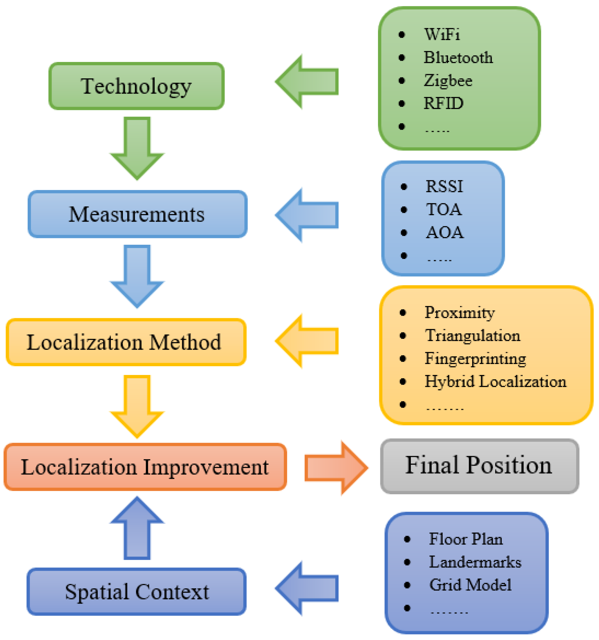
In this section, we introduce the design of our indoor short-range localization system. The details of the different components are introduced with specific reference to the workflow presented in
Section 2.2. Specifically, we present our choices regarding Technology, Measurements, Localization Methods, Spatial Context and Localization improvement.
3.1. Technology: Bluetooth
In our system, we decided to adopt Bluetooth as the wireless technology. Bluetooth beacons have been demonstrated to be effective for the implementation of indoor localization systems, e.g., [
11], also guaranteeing low power consumption, especially considering the last BLE revision. This feature allows boards equipped with small batteries to emit beacons, thus also enabling their installation on small objects. In this work, we demonstrate that BLE is suitable for short-range localization via a set of preliminary experiments that are presented in
Section 4.1.
An indoor localization system based on BLE is composed of one or more receivers and a tag node installed on the object. The tag periodically emits a Bluetooth beacon that is received by the readers. Each reader can analyze multiple data, including the RSSI value, the Media Access Control (MAC) address of the tag, and the reception timestamp. In the literature, a different configuration has also been proposed: fixed nodes are installed in a certain environment programmed to emit beacons, while the target node, typically a mobile node, analyzes the beacons to derive its position. This configuration, however, is more suitable for contexts where the mobile device is a fully fledged device, e.g., a smartphone, that is able to analyze the signal from the beacons for positioning. In our case, we decided to keep the device installed on the object as simple as possible and move the complexity to the readers, which is assumed to be a powerful device. This reduces the cost of the tag, thus allowing its installation on the products of the assembly line on a large scale. In addition, BLE tags that emit beacons for positioning or information broadcast have already been demonstrated to be energy efficient, thus also representing a viable solution in the case of battery-powered devices. For instance, in [
12], it is shown that a BLE tag that emits a beacon every 800 ms can have a lifetime of 640 days if equipped with a CR2477 battery with dimensions of 24 × 7.7 mm and a capacity of 1000 mAh.
3.2. Measurement: RSSI Preprocessed with Kalman Filter
As with many other solutions from the literature, our localization system analyzes the beacon RSSI measured by each receiver. RSSI is a metric that measures the Received Signal Strength (RSS) with Formula (
1), i.e., the actual signal strength received at the receiver measured in decibel milliwatts (dBm). RSSI can be used to estimate the distance between a transmitter (Tx) and a receiver (Rx): the greater the RSSI value is, the smaller the distance between Tx and Rx. The absolute distance can be obtained by exploiting a signal propagation model, e.g., a simple path loss propagation model that estimates the distance
D between Tx and Rx, considering a known reference value:
where
n is the path loss exponent, which varies from 2 in free space to 4 in indoor environments, and
is the
value of a reference distance, e.g., 1 m, from the receiver, which is known.
Unfortunately, RSSI is a noisy measurement, especially in indoor environments, due to the obstacles and multipath fading. Therefore, to improve the signal quality, in our system, we decided to adopt a Kalman filter to filter the RSSI values. This practice is already used in many localization systems [
13,
14,
15].
The Kalman filter estimates the state of a process where the state is difficult to measure due to many sources of noise. The state at the i-th step is given by the following linear stochastic equation:
where matrix
A relates to the state of the previous step
i − 1 with the state of the current step
i; matrix
A can change step by step. Matrix
B, instead, relates to the control input
u to the state
x. The measurement is called
and can be calculated with
where matrix
H relates to the state of measurement
z at step
i. Matrix
H can change step by step as well. The terms
and
are two random variables, respectively: the process noise and the measurement noise. They are assumed to be independent of each other and both have a normal probability distribution that is
and
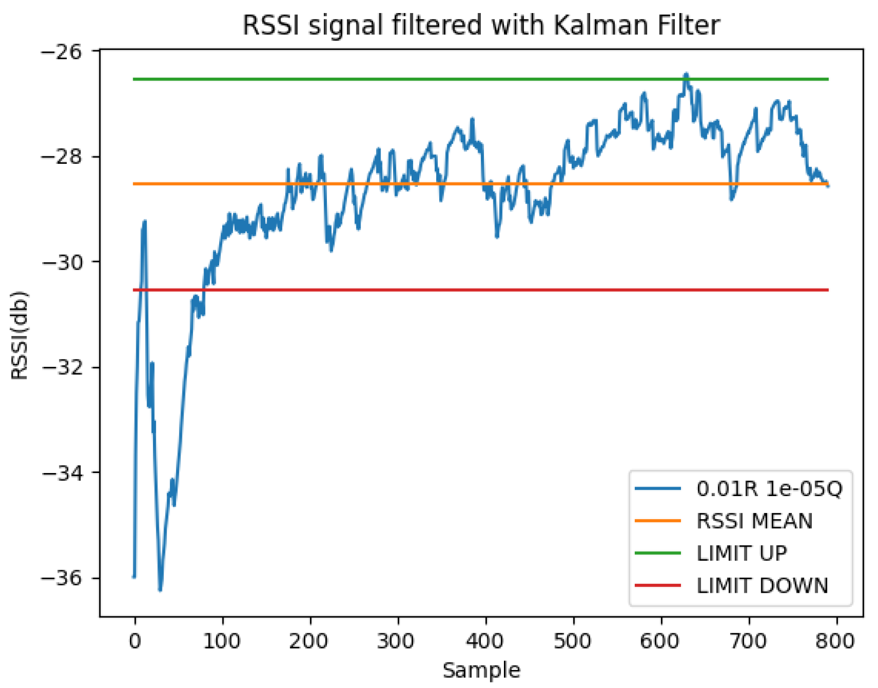
. Q and R are the covariances of the process and measurement noise, respectively, and are two parameters that can be adjusted. After adjusting these two parameters, the filter changes its behaviour: it is more confident in measuring the expected value; however, additional latency is introduced.
In [
16], the filter behaviour with different values of Q and R is analyzed. In a typical configuration, the Kalman filter is used with its default parameters, i.e., Q is set to 0.00001 and R is set to 0.01. In this work, an assessment of different configurations for the Kalman filter parameters is performed in order to confirm the Q and R settings for the short-range indoor localization scenario considered. Details on this analysis are reported in
Appendix A.
3.3. Localization Method: Fingerprinting
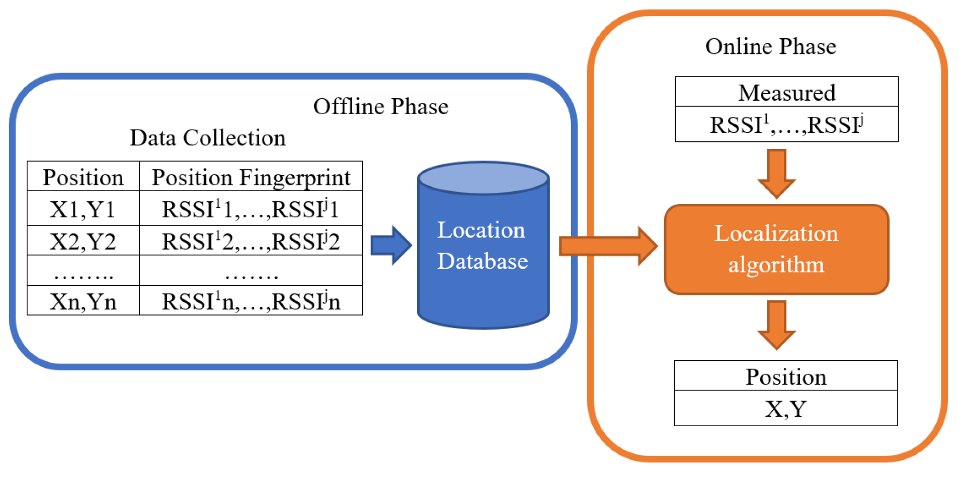
In our system, we adopt a fingerprinting-based localization method. Fingerprinting-based localization consists of two phases, as shown in
Figure 3: an offline phase and an online phase. In the offline phase, measurements are collected on a set of predefined locations: the readers are placed in fixed locations, generally in strategic positions such as in the 4 corners of a room, while a tag that emits periodic beacons is moved from one predefined location to another, after remaining in one location for a certain period of time in order to allow the readers to receive a sufficient number of beacons and collect the values of the RSSI. The RSSI samples are combined by a central node, based on the timestamp, and the position of the tag. This phase results in a training set, which creates the fingerprint database.
In the online localization phase, instead, readers collect data in real-time and transmit the RSSI samples to a central node, which compares such samples with the data stored in the fingerprint database to estimate the location of the target, via a specific localization algorithm.
3.4. Spatial Context: Grid Model
In this specific use case, our localization system considers as spatial context a rectangular surface, which represents an assembly line where multiple workstations are located. To identify the product with high precision, the surface is divided into a grid, in which different positions where the object can be placed are identified. In our localization system, we assume that the precise location inside each workstation is not tracked, as we aim only at identifying the current workstation where the product is located.
3.5. Localization Improvement
At the core of every localization solution, we have the localization algorithm that is implemented on the central node. The algorithm takes as input the data from fingerprinting and calculates the final position, also considering spatial context information. In the literature, many approaches have been considered. In this work, we assess the performance of multiple solutions with limited complexity in order to make their implementation feasible on an embedded system with limited computing resources: regressors, CNN and RNN.
For the regressors, we consider the following approaches:
Decision Tree (DT): The decision process is represented by a tree where each node is a conditional function. Each node checks a condition (test) on a particular property of the environment (variable) and has two or more down branches in operation. It always starts at the root node, the parent node located higher in the tree, and proceeds downwards until it reaches the leaves. According to the values detected in each node, the flow takes a different direction. The final decision lies in the terminal leaf nodes, i.e., the lower ones. The main advantage of logical trees is their simplicity: they are easy to understand and implement. Compared to neural networks, decision trees are easily understandable by humans; therefore, a man can verify how the machine reaches a certain decision. The main disadvantage of the decision tree representation is that it is not suitable for complex problems, as it can only describe a relationship between a truth function and logical combinations of attributes.
Random Forest (RF): The random forest algorithm is a technique that involves the use of many decision trees. Each tree in the forest generates classification predictions. When all the decision trees have a forecast, a collective decision is made with the highest number of votes, becoming the forecast of the entire model. The advantage of using the random forest is to introduce a randomness factor to mitigate the overfitting of the training set concerning decision trees. The disadvantages, compared to decision trees, are that the performance does not always increase with the number of trees, the complexity of human interpretation of the choices made by the random forest, and the need for a greater number of samples for training.
K-Nearest Neighbors (KNN): This algorithm exploits the characteristics of the samples in training to classify a new value. A sample is ranked by the distance from its neighbors, with the sample assigned to the most common class among its k closest neighbors. The number of samples to use is a parameter of the algorithm, while the distance can be any metric, although the most common choice is the standard Euclidean distance. Neighbors-based methods are known as non-generalizing machine learning methods, as they simply remember all their training data, eventually transformed into a fast indexing structure with some algorithms. Based on how the weights of the choices are fixed, we can have a uniform KNN that assigns equal weights to all points, or a distance KNN that assigns weights proportional to the inverse of the distance from the point.
As several studies have shown, the use of artificial intelligence (AI) has become a game changer for several sectors such as industry, healthcare, and finance [
17]. In light of this, we propose the exploitation of CNNs and RNNs in comparison with traditional regression methods. For the CNN we select different models that were initially defined to solve similar problems for indoor localization. The models considered, for both CNNs and RNNs, are not pretrained for our use cases. We report on the training in
Section 5.2 with the data collected specifically for our indoor localization fingerprinting system:
AlexNet: It is one of the most popular CNN used for image classification, [
18]. AlexNet is a convolutional neural network architecture that in 2012 won the Imagenet Large-Scale Visual Recognition Challenge, ILSVRC. The network was trained with over 1.2 million HD images, characterized by 60 million parameters and over 600,000 neurons, for a total of about 1000 possible classifications. The model includes 5 convolutional layers, some followed by MaxPooling layers and 3 fully connected layers.
ResNet50: This is another popular CNN used for image classification, [
19]. ResNet, in 2015, managed to unseat AlexNet from first place in the ILSVRC by winning the competition. The reason for this victory was due to the intuition that very often the performance deteriorates when the depth of the network increases. In order to overcome this issue, the authors introduced the concept of Residual Block: in traditional networks, layers propagate outputs as inputs to the next layer; in networks with residual blocks, layer n propagates the results to the next layer, therefore n + 1 and to layer n + 2, and so on, thus mitigating the vanishing gradient problem.
Liu CNN (hereafter
Liu for short): The authors of [
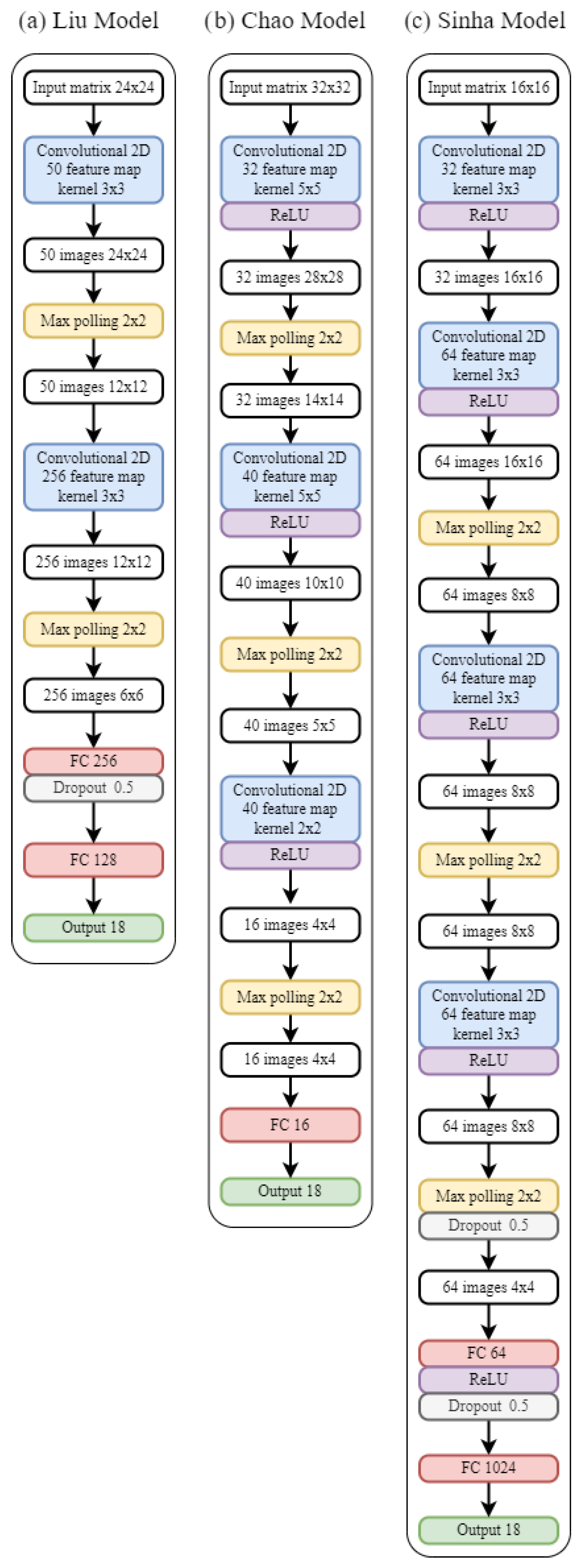
20] propose a CNN for indoor localization based on a hybrid wireless fingerprint of the Bluetooth and Wi-Fi signal. This CNN is used to analyze a spatial image composed of the signal collected from several access points. Unlike AlexNet and ResNet50, this network is much shallower and is therefore better suited for real-time applications.
Figure 4 shows the network structure. In order to exploit this CNN in our use case, we performed minor modifications, specifically in order to adapt the original CNN to the 18 outputs that are our reference points.
Chao CNN (hereafter
Chao for short): In [
21], a CNN-based localization approach for locating RFID tags is presented. The authors try to exploit both the joint fingerprint characteristics of the RSSI and the arrival phase difference (PDOA). The proposed CNN has 3 levels of convolution and 3 of pooling, where normalized RSSI and PDOA data are formed into images as input to train weights in the offline phase of the fingerprint technique. In the online phase, the RSSI and PDOA data of the test tags are collected and then the locations of the unknown tags are predicted based on the CNN output. Additionally, in this case, some minor modifications to the original CNN were applied, as shown in
Figure 4. Specifically, in our case, the CNN was modified in order to extend the number of input and output points to 18, according to the reference points adopted in our use case.
Sinha CNN (hereafter
Sinha for short): The authors of [
22] present an architecture for indoor localization using the Wi-Fi signal. To this aim, they present a CNN model based on the RSSI dataset of Wi-Fi access points. The model is mainly based on convolution and Relu layer pairs, as shown in
Figure 4. The experimental results reported in [
22] show that the proposed model can achieve an accuracy of 94% while also achieving better performance than AlexNet and ResNet.
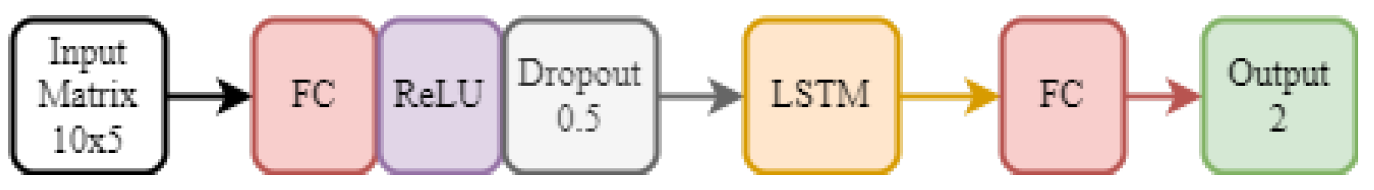
For the RNN, we chose the method proposed in [
23], which uses LSTM networks to learn the complex temporal patterns of signal power measurements and estimate the user’s position in real time.
Figure 5 shows the proposed structure with one FC layer and one LSTM layer because it is the best configuration to achieve a lower error average (1.92 m).
4. Testbed Implementation and Data Collection
In this section, we first introduce the results obtained from a preliminary set of experiments aimed at validating the signal profile of BLE for short-range localization (
Section 4.1), and then we present our testbed for short-range localization (
Section 4.2). The section is concluded with an introduction to the data collection methodology we used to create a dataset for the training and validation of different methodologies for short-range localization (see
Section 4.3).
4.1. BLE Signal Profile for Short-Range Localization
As highlighted in
Section 2.2, other studies have already adopted BLE for localization. Some of those studies have also already profiled the RSSI over distances, e.g., in [
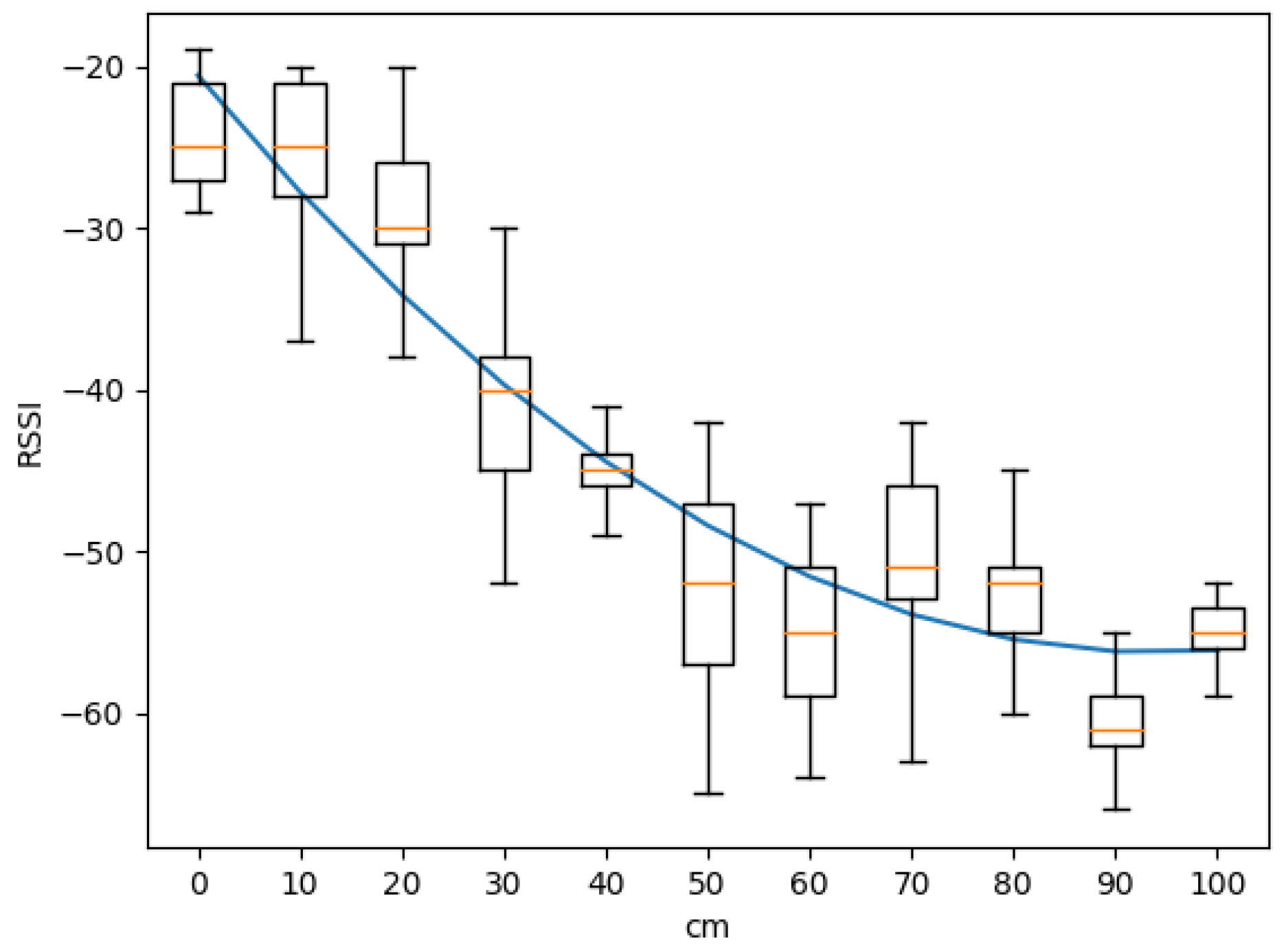
11], the trend curve of the RSSI w.r.t. distance is analyzed. However, they do not include an accurate resolution short distance, as in our case. In order to verify that BLE is also suitable to track distances below 1 m, we ran a set of preliminary experiments to derive the RSSI profile with short-range distances.
To this aim, we placed a single BLE receiver installed under a table, while a beacon emitter was moved at increasing distances from the receiver, i.e., between 0 and 100 cm with 10 cm steps. For each point, 300 samples were collected.
Figure 6 reports the RSSI values obtained on each position and the corresponding fitting curve. These results show that when the distance is below 70 cm, the trend line of the average values has a linear slope; after 70 cm, the average values of the RSSI fluctuate around the value of −55 dBm. This makes it more difficult to analyze the RSSI value and find a correlation between distance and RSSI.
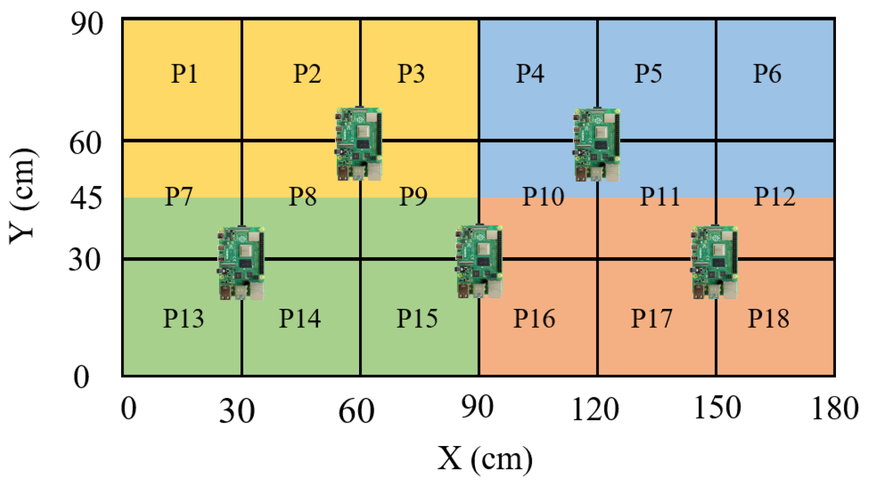
These results indicate that in order to ensure fine-grained positioning, the readers must be placed so any point in the area has at least one reader that is at a distance less than 0.7 m. To this aim, we derived the positioning scheme reported in
Figure 7. The reader nodes are placed under the surface with a specific pattern, which is optimized to maximize the coverage of the area with a minimal number of readers. This scheme ensures that for every point in each position, we have at least one reader that is at a distance less than 0.7 m. The overall area is composed of a grid of 18 positions, marked as
, with
in the figure. The area is assumed to be devoted to four different workstations, highlighted with four different colors.
4.2. High-Level Architecture
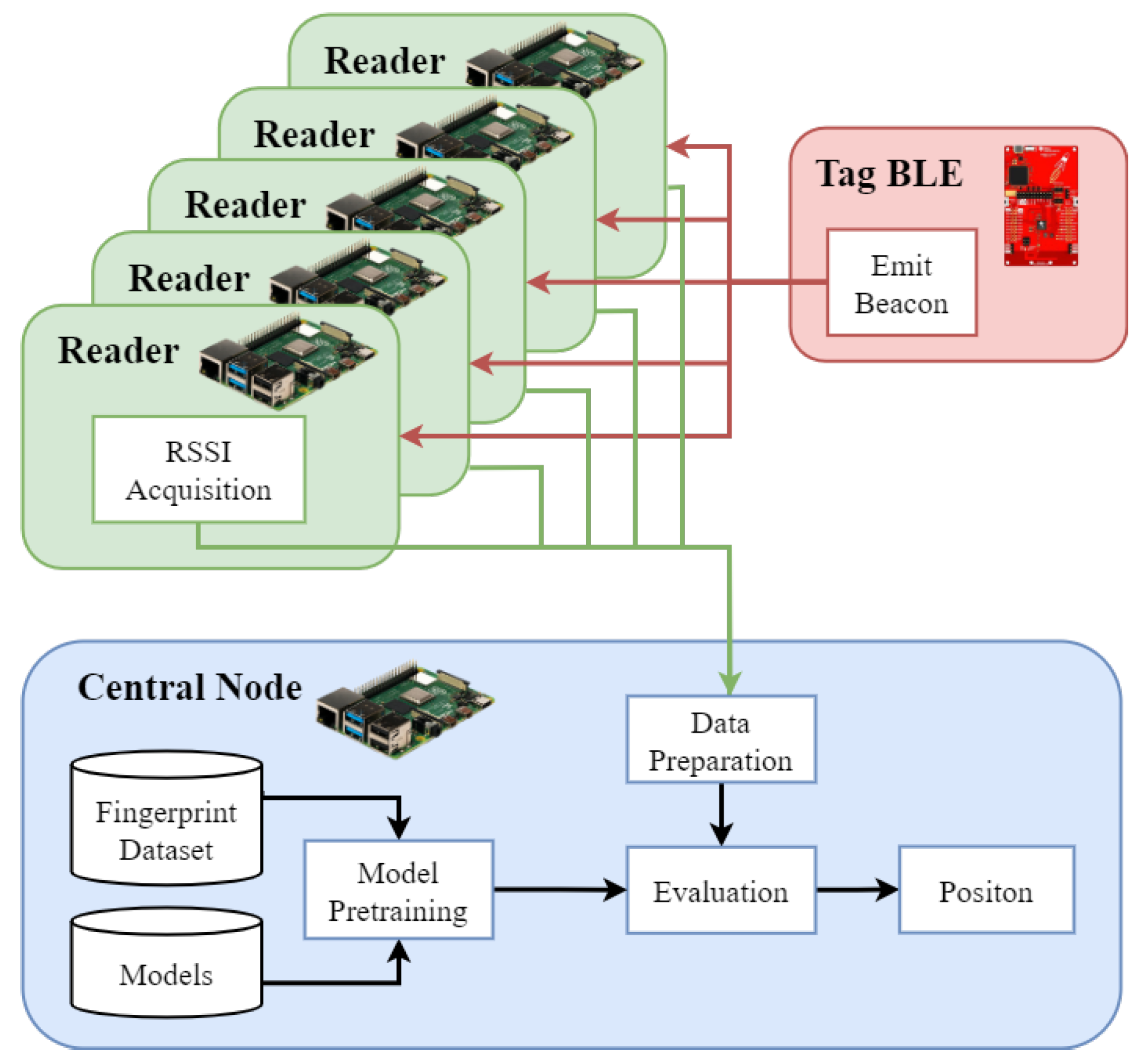
Figure 8 shows the overall architecture of our testbed. The system comprises three main components: a BLE tag, five readers, and a central node. The BLE tag is attached to the moving product and emits a beacon periodically. The beacon is received by the readers that can measure the RSSI value.
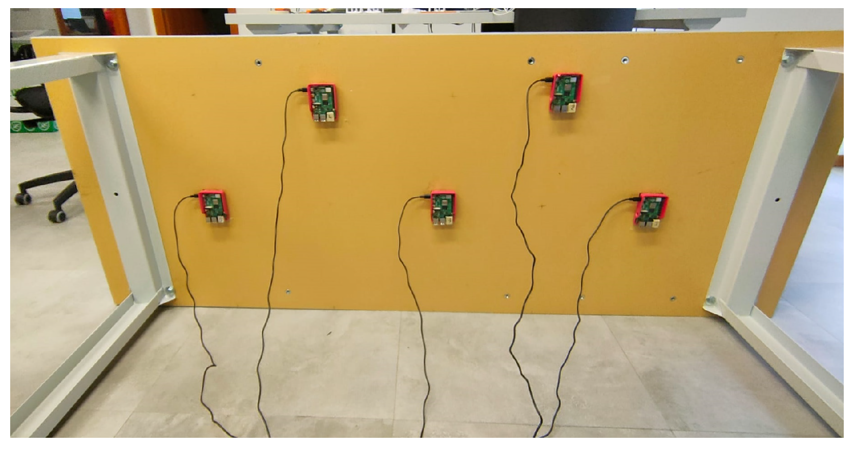
The central node analyzes the data collected by the readers, implementing one specific analysis model. When a model is selected, it is used to analyze the RSSI values received from the readers, also including the data preparation phase, such as filtering via the Kalman filter. Eventually, the data are processed and the position of the BLE tag is returned. In order to create a realistic dataset, we implemented the testbed in an environment that emulates a portion of the production chain, i.e., a smart workbench where one or more production stations are placed. The workbench is a 1.8 m × 0.9 m table, while a grid is composed of 30 × 30 cm rectangles considered for object location, thus resulting in a 3 × 6 grid of possible positions. In order to collect the beacon signal from the tag in a fine-grained manner, we used five Raspberry PI v4 embedded boards (Raspberry PI v4 website:
https://www.raspberrypi.org/products/raspberry-pi-4-model-b/, accessed on 8 Ocotber 2023) as readers that were installed under the workbench, as shown in
Figure 9.
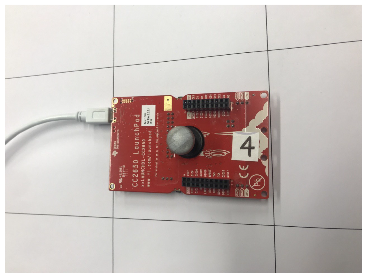
The boards were installed under the surface in order to minimize the interference with the workers or machines operating on the surface, while their placement was designed specifically with a modular pattern, which can be repeated as the surface expands to cover larger working areas, e.g., in a production line. The LAUNCHXL-CC2650 board from Texas Instruments (LAUNCHXL CC2650 website:
https://www.ti.com/tool/LAUNCHXL-CC2650, accessed on 8 Ocotber 2023) was used as a tag. The CC2650 wireless MCU is equipped with a 32-bit ARM Cortex-M3 processor that runs at 48 MHz as the main microcontroller and a rich peripheral feature set. Our proposed system then consists of 6 Raspberry Pi 4 costing EUR 50 per unit and one LAUNCHXL-CC2650 costing EUR 50. Our system therefore has a total cost of about EUR 350. Thus a much lower price relative to the cost of commercial UWB indoor tracking systems of USD 1999 (
https://estimote.com/spacetimeos, accessed on 8 Ocotber 2023).
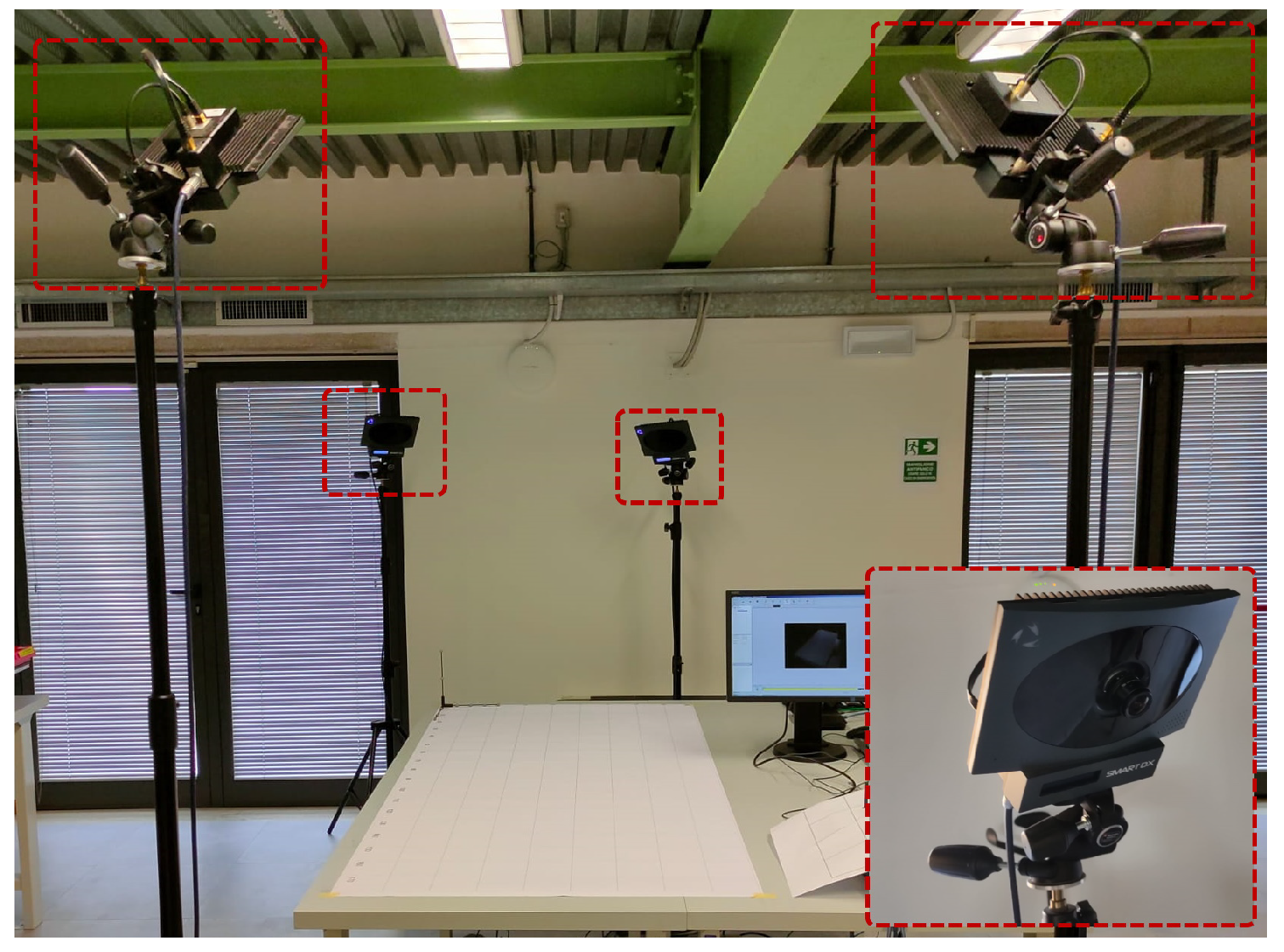
In order to have a reference system of the tag’s absolute positions (i.e., our ground truth), we used a commercial infrared camera system for high-precision localization. Specifically, we adopted BTS Bioengineering’s BTS SMART DX 100 (
https://www.btsbioengineering.com/products/smart-dx-motion-capture/, accessed on 8 Ocotber 2023) with four high-resolution infrared cameras that can ensure localization with an accuracy of 0.2 mm and a maximum capture rate of 280 FPS. In our case, the system is configured to collect data with a frequency of 100 Hz. The four cameras are positioned at the corners of the table, as shown in
Figure 10.
Figure 11 shows the Bluetooth beacon that was used in our tests with a marker that is tracked by the camera system just described.
This position guarantees data collection even when one of them is obstructed by the operator. In order to synchronize data from the ground truth system and the different readers, synchronized timestamps were used. To this aim, the Network Time Protocol (NTP) was exploited to synchronize the clock of all the hosts involved.
4.3. Dataset Creation Methodology
To start, we carried out a data collection phase to create a dataset for the training and validation of different localization methodologies. To this aim, a BLE tag, emitting beacons at the frequency of 10 Hz, is moved manually on the testbed to cover different positions on the grid shown in
Figure 7. For each position, RSSI samples are collected by the 5 different readers before moving to the next position. For each position, the exact coordinates (x,y) are collected via our reference system. Each sample in our dataset contains five RSSI values, e.g., RSSI-r1, RSSI-r2, RSSI-r3, RSSI-r4, RSSI-r5, with one from each reader, plus the exact location, e.g., x, y, and a timestamp.
RSSI is known to be a very noisy signal: as the current environment changes, the signal can change as well due to variations in the interference or changes in the environment that can cause different reflections. In order to reflect this variability in our data, the testbed was placed in a laboratory environment with industrial equipment (e.g., robots) and other devices (Wi-Fi or BLE devices) that can generate interference. In addition to this, the data used for testing was sampled over multiple days, in order to collect samples under different interference conditions, i.e., different days and hours of the day.
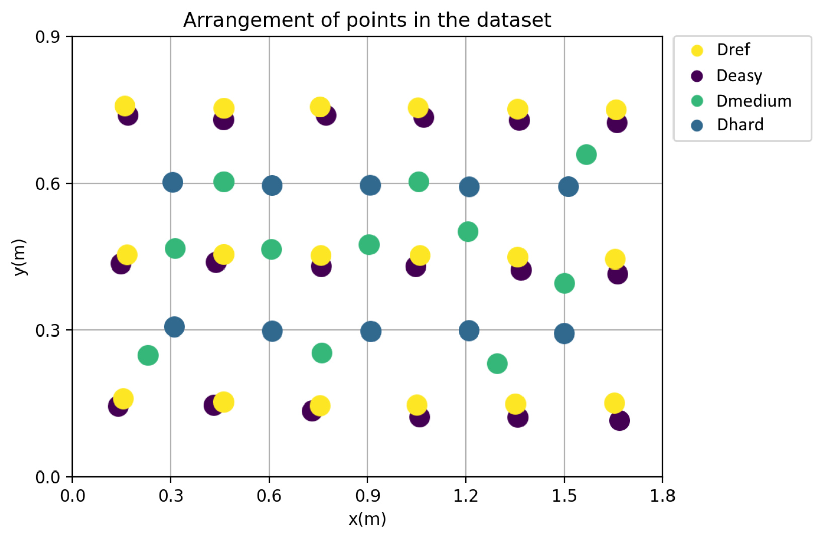
Overall, four different datasets were collected, i.e., Dref, Deasy, Dmedium, and Dhard. Each dataset includes a different set of positions on the grid. A graphical representation of the positions considered for the creation of each dataset is reported in
Figure 12.
As shown in
Figure 12, two datasets were collected in a more systematic way: Dref and Deasy were taken in the middle of the position. Instead, in order to obtain an idea of how our system behaves in real-life situations, we constructed two paths, Dmedium and Dhard, that have a non-predetermined pattern and thus reproduce a semi-random movement of the BLE tag on our assembly line. This allows us to see what happens even in borderline cases in which the beacon is in between two or more positions.
Table 1 shows the number of samples collected for each dataset, respectively, 8814 for Dref, 5985 for Deasy, 3591 for Dmedium, and 3040 for Dhard, with a total of 21,430 samples overall. Dref was used for the offline training of the fingerprinting technique, while the other datasets were used for testing and validation. Each dataset was collected on different days to provide a greater variety of external factors. Furthermore, as shown in
Figure 9, the devices are in a non-line-of-sight condition so these datasets already present this issue needing to be resolved.
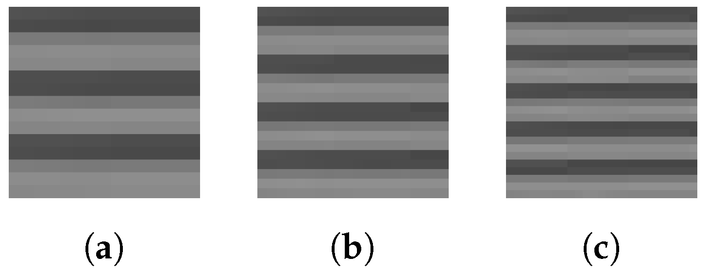
While Dref is collected by placing the tag in the center of each square of the grid, the others adopt different positioning schemas with increased localization difficulty. Deasy is used to validate the positioning systems with data that are close to the positions included in Dref, i.e., when the object is placed in a position nearby the exact center of each square. The other datasets, instead, include other challenging positions, i.e., positions that are at the border of a workstation to simulate an object temporarily placed aside (e.g., during assembly operations), e.g., Dmedium simulates an object placed at the border of a station in close proximity of the border between two different positions, while the Dhard dataset simulates an object placed in proximity of the corner of a station, i.e., close to the corner of three positions. It is important to highlight that the Dmedium and Dhard datasets contain infrequent positions where an object might be placed only temporarily. The goal of these datasets is to understand if the system is robust enough to detect infrequent positions that were not included in the initial set. In our evaluation, we also use the union of the three test datasets, i.e., Deasy, Dmedium, and Dhard. Hereafter, we refer to it as Dall. For each dataset, an image dataset is created to be used for the models examined. To create the images for training and testing the CNNs and RNNs, we converted the collected data into matrices. Each image is created based on the RSSI values arranged as in the following matrix:
where
h is the height of the matrix, and
w is the width of the matrix. Thus, the RSSI values are arranged vertically. More than one size of the matrix is generated, and that is the parameter of the specific CNN. The sizes chosen for the matrix are:
15 × 15: that reports 45 samples of RSSI from each reader.
20 × 20: that reports 80 samples of RSSI from each reader.
25 × 25: that reports 125 samples of RSSI from each reader.
To build more matrices to augment the data, and take into account a possible temporal correlation, a window was also considered to take the RSSI values of 10 samples, which results in 1 s. The matrix is then converted into an image in grayscale, with the values of the normalized RSSI multiplied by 255, and then the different dataset is constructed. In
Figure 13 and
Figure 14, we show some examples of RSSI matrices converted into images.
5. Results
In this section, we present the results of the performance evaluation. Specifically, in
Section 5.1, we present the results obtained with the regressors, while in
Section 5.2, the results obtained with the CNN and in
Section 5.3, the results obtained with RNN are presented. We conclude with a final comparison where the best solution for each technique is considered and analyzed in
Section 5.4.
In order to handle the high-frequency fluctuations that characterize RSSI measurements, the Kalman filter is used with its default parameters, i.e., Q is set to 0.00001 and R is set to 0.01, which are confirmed as also resulting in good performance in the short-range localization use case, as shown in
Appendix A.
To compare the performance of the regressors, we use the empirical cumulative distribution function (ECDF) of the error. Two different error metrics are considered: (i)
discrete error, defined as the difference in terms of positions between the predicted position and the real position in the grid; and (ii)
continuous error, defined as the Euclidean distance between the real position (
,
) and the predicted position (
,
). The discrete error is the metric that aligns most closely with our intended application, as it directly quantifies how accurately the proposed system identifies the correct station where the object is situated. On the other hand, we measure the continuous error to obtain a more detailed assessment, especially valuable since, in certain scenarios, the distinctions between various methods in terms of discrete error are relatively small. Moreover, the continuous error provides a means to gauge the resilience of the proposed solution across all scenarios where the worker does not position the object precisely at the center of the working area, as exemplified in the Dmedium and Dhard datasets.
For the discrete error, we use Formulas (
5)–(
7): we calculate the error made on the
x-axis (
5) and
y-axis (
6) as the absolute value of the difference between the predicted index (
or
) and the correct one (
or
). From these two calculated errors, i.e.,
and
, we select the greater as a discrete error. The continuous error, instead, is calculated using Equation (
8).
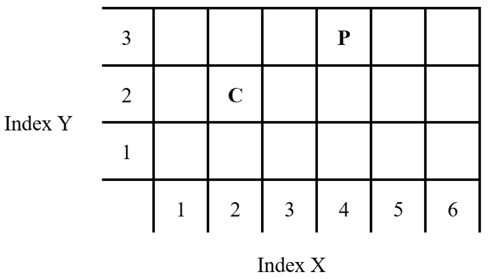
Figure 15 shows an example of a bad prediction. The position of the object is indicated with C and has coordinates [2,2]; the prediction, instead, indicated with P, has coordinates [3,4]. The calculation of Formulas (
5) and (
6) give us a value of
equal to 2, while
is equal to 1. By applying instead Formula (
7) using
and
, we find that the error is equal to 2.
5.1. Regressors’ Performance Evaluation
In this section, we present the results obtained with the regressors. We trained the regressors using the same dataset as a training set, i.e., the Dref dataset that was used 90% for training and 10% for validation. The remaining datasets, instead, were used to test the performance of the system. To this aim, on each dataset, the cumulative distribution function of the continuous distance error and the discrete error were calculated and reported in the following.
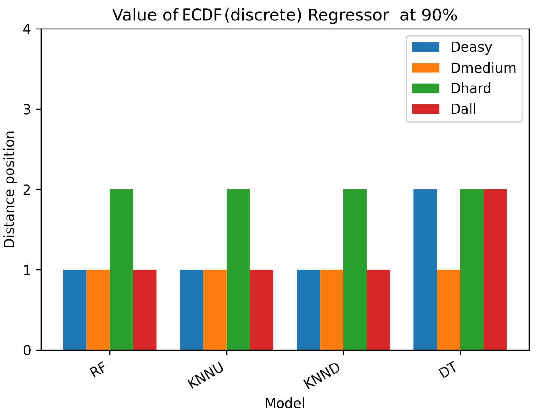
Figure 16 shows the error of the ECDF at 90% in the case of the discrete position for all the regressors. The results obtained with the Deasy, Dmedium, Dhard, and Dall datasets are reported. The 90% ECDF was adopted since it can provide a rough measurement of the precision, valid for a wide range of non-safety critical applications. A similar approach was adopted in [
24] for the analysis of a localization system based on the fusion of smartphone inertial data and Bluetooth beacon data. As we can notice, we have no significant differences between RF, KNNU, and KNND, i.e., all the regressors result in similar behaviour with the four datasets. Instead, DT reports a higher error even with the Deasy dataset, the less critical dataset.
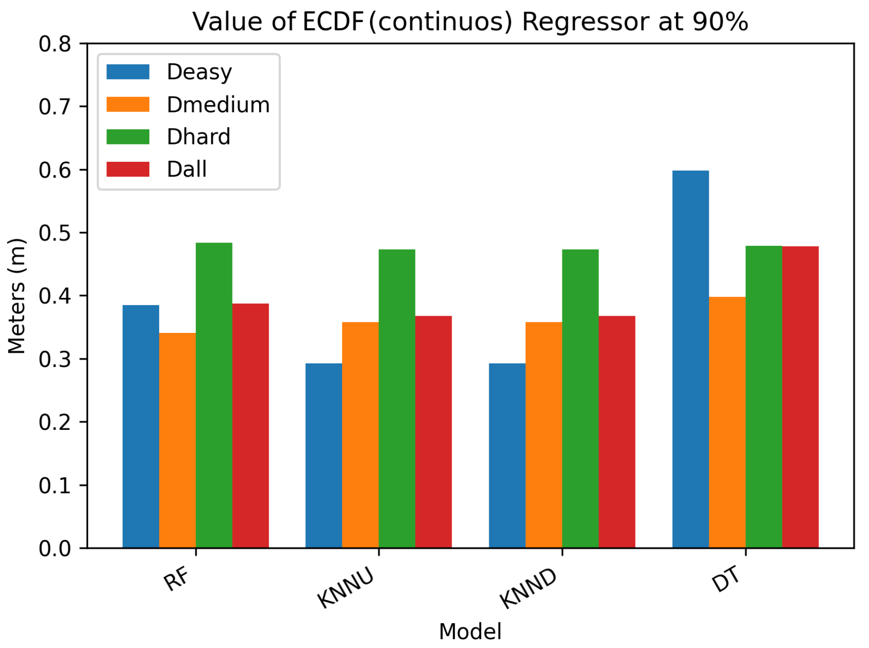
To better analyze the differences with the regressors, we also analyze also the continuous error.
Figure 17 shows the ECDF of the continuous error at 90% for all regressors. In this case, we can notice that the four regressors behave differently: RF results in a larger error in Deasy, while KNNU and KNND have comparable results. In general, as expected, as the difficulty of the dataset increases, the error increases as well. Moreover, in this case, DT results in the highest error. These results show that KNND slightly provides the lowest error on Dall; consequently, it is used as a term of comparison in the final analysis in
Section 5.4.
5.2. CNN Performance Evaluation
After analyzing the performance of different regressors, in this section, we examine the performance of different CNNs. As introduced in
Section 3.5, five CNNs were selected. For each model, we considered two configurations, the CNN used with the data filtered via Kalman and the CNN that uses the raw data directly. The goal is to assess if the filtering of the data used for training can help to improve the performance, considering that CNNs can already handle some degree of noise since they were designed mainly for image analysis. The labels that end with “_k” are associated with the configuration where the Kalman filter is used, while the labels that end with “_nok” are with the Kalman filter disabled. In order to guarantee the best performance for each CNN in our use case, their hyperparameters were tuned using a grid search in the ranges shown in
Table 2. This preliminary analysis identified the hyperparameters reported in
Table 3 as the best configuration for each CNN.
The output of any CNN is a matrix of probabilities associated with each position on the grid. In order to calculate the predicted position from such a matrix, we used the following formulas:
where
is the probability that the tag is in the
k-th position, while
and
are the coordinates of the
k-th position.
The number N, i.e., the number of output points taken into account, is varied in the range [1, 18] to assess how it influences recognition performance. Our preliminary results showed that all networks improved their accuracy from setting N to 18; consequently, we used this value for our experiments.
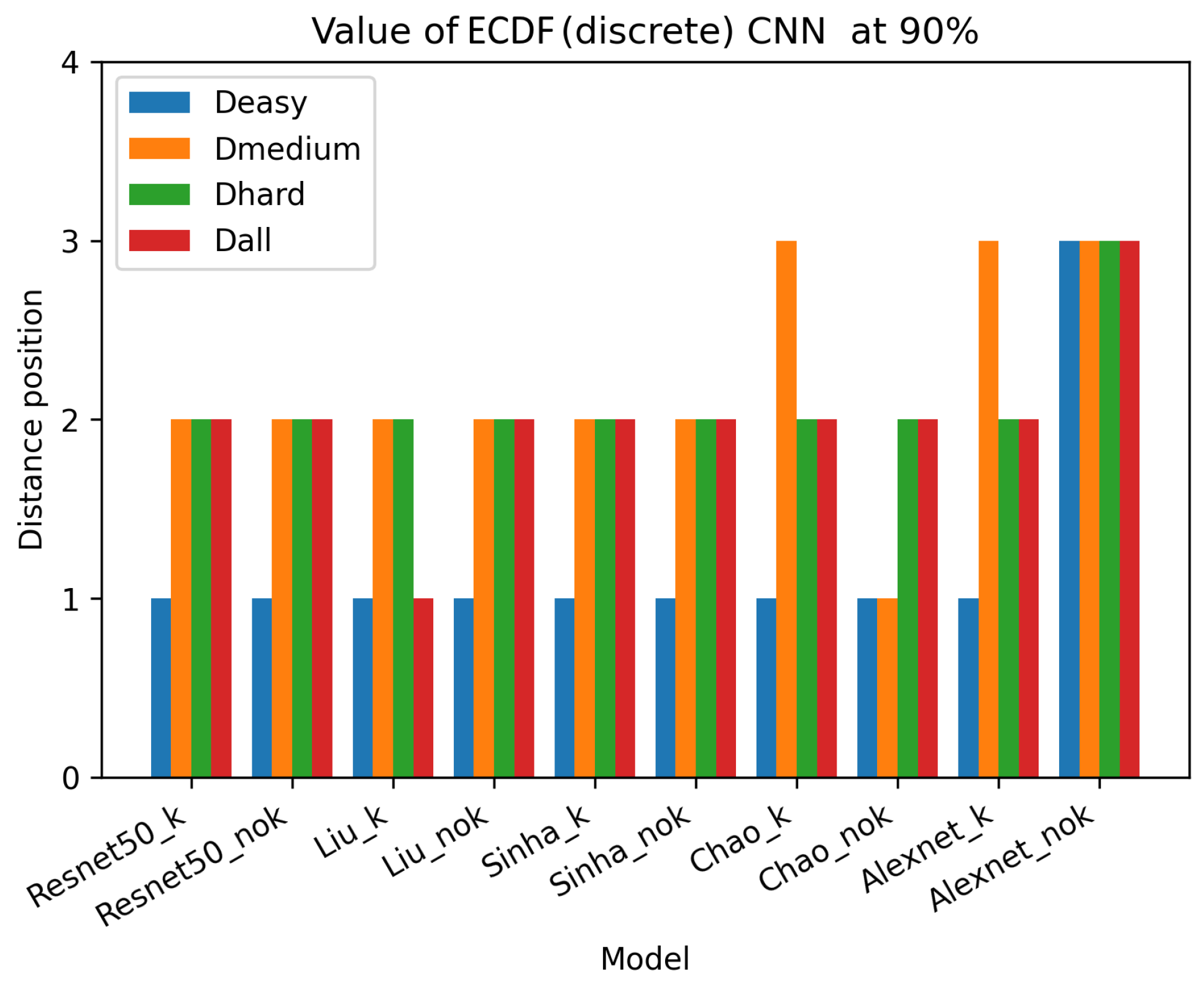
As already performed for the regressors, we carried out different experiments with different datasets and we analyzed both the continuous and discrete errors. In
Figure 18, the ECDF values at 90% of the discrete error are reported for the considered CNNs. From these results, we notice that also in this case, as happened with the regressors, we have networks that behave similarly. The two best networks are Liu_k and Chao_nok, with the former, in particular, having only a one-position error with two datasets and a two-position error with the others.
As for the regressors, it is difficult to assess the performance in the discrete case, while more noticeable differences are displayed in the continuous case.
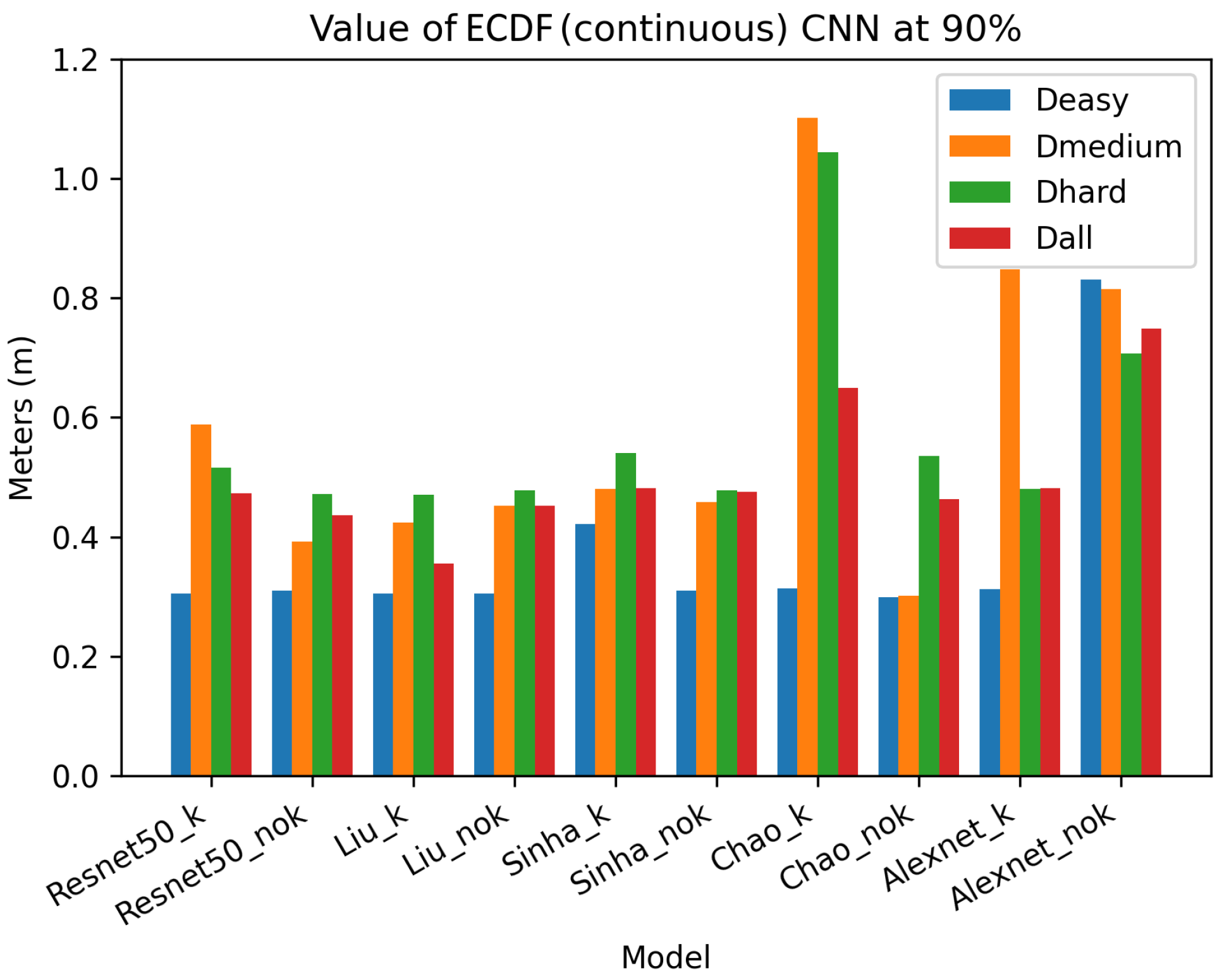
Figure 19 shows the ECDF values at 90% of the continuous error of the CNNs. These results show that the best network, in terms of performance, is the Liu_k, which obtains a 0.35 m error on the dataset Dall. If we compare the results obtained with and without the Kalman filter, we can notice that the filter does not always improve the performance of the CNN. For example, the AlexNet model results in an error for the Dall dataset that is 0.75 m without Kalman and 0.48 m with the Kalman filter. The other models, such as the Chao model, have different results, e.g., 0.65 m without Kalman and 0.46 m with Kalman. Therefore, the use of the Kalman filter does not always result in better performance. Further considerations can be made about the poor performance of Alexnet_nok. We think that these results are not due to the input image size both Resnet_nok and AlexNet (both the versions) have input images of 20 × 20 and were trained with the same dataset. Furthermore, looking specifically at the graphs, we see that Alexnet_k has comparable results to the other models examined. We, therefore, consider them to be comparable tests.
5.3. RNN Performance Evaluation
In this section, we analyze the performance of RNNs. As for the other solutions, the RNNs are trained using the Dref dataset for training. Two RNN configurations are considered, one with the data filtered with a Kalman filter and one using the raw data. The results for the former configurations are reported with the name “RNN_k”, while the results obtained with the latter are reported with “RNN_nok”. After training, the other three datasets are used as test datasets to perform the performance study, as for the other solutions considered in this paper.
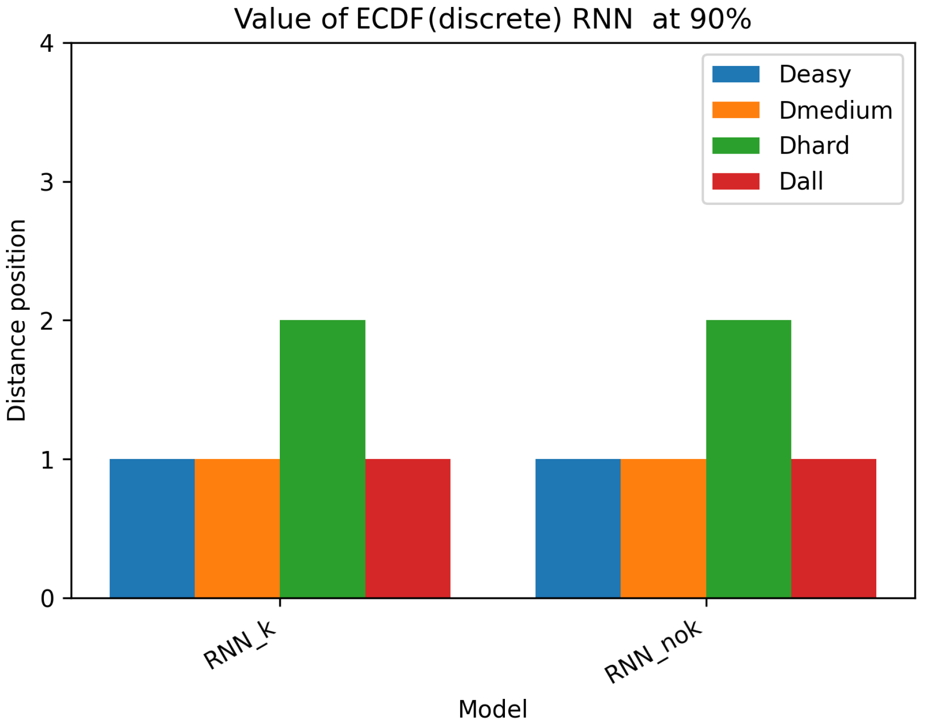
Figure 20 shows the values of the 90% ECDF for the discrete error. As can be seen, both networks result in similar performance.
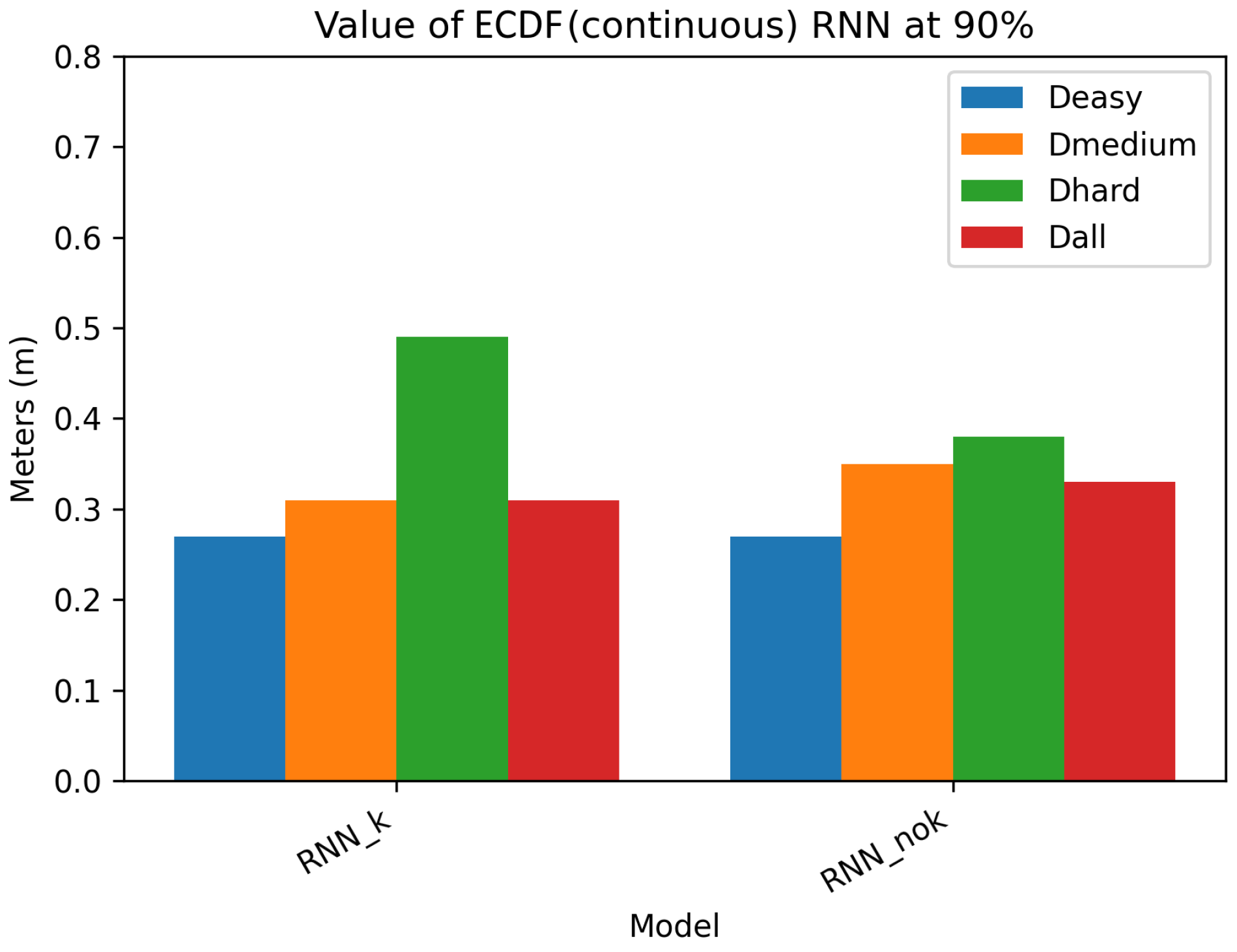
Figure 21, instead, reports the ECDF at 90% of the continuous error. In this case, we obtain different results with different datasets. The RNN_nok results with the Dhard dataset show an error of 0.38 m, while RNN_k reports an error of 0.49 m. The results, however, are different if the Dmedium dataset is considered: the RNN_k reports an error of 0.31 m, while the RNN_nok has an error of 0.35 m. In order to identify the most suitable configuration, we can consider the results obtained with the Dall dataset: the RNN_k results in an average error of 0.31 m, while the RNN_noK results in 0.33 m, although the difference in this case is also minimal. We use the RNN_k as the term of comparison in our final analysis since it obtains better results on the Dall dataset.
5.4. Final Comparison
In this section, we carry out a final comparison. To this aim, the configuration that resulted in the lowest continuous error was selected for each category in order to make a final assessment. Specifically, for the regressors, we consider KNND, for the CNNs, we consider the Liu_k network, while for the RNN we consider RNN_k.
The goal is to analyze their performance more in depth with the Dall dataset and draw some final conclusions and guidelines.
In this final assessment, we consider the ECDF at 80%, 85%, and 90% for an exhaustive assessment of the error.
Table 4 shows the ECDF values for both discrete and continuous errors for KNND, Li_k, and RNN_k.
If we consider the discrete ECDF, we notice that all the models result in an error of 1 position in the grid system we considered in our experiments. This shows that all the models result in a minimal error in recognising the position on the grid.
If we consider the continuous ECDF, we notice that different methods result in different errors. The minimum error for each configuration is highlighted in bold. As can be seen, the RNN_k has the lowest values at 80%, 85%, and 90% with errors of 0.23 m, 0.28 m, and 0.31 m, respectively. Even though the difference in performance across the methods is in the order of centimeters, these results confirm that RNN_k is the approach that performs best in the considered use case.
In order to compare the error obtained using the proposed system with the literature, even if a direct comparison is not possible, a comparison of the order of magnitude can help to assess the improvement in the level of precision obtained with our configurations. In [
20], the authors obtained an average error of 3.91 m using a CNN based on the one proposed by Liu, while they obtained an error of 4.17 m error using a KNN. In our case, the CNN proposed by Liu resulted in an error of 0.35 m on average. In [
21], the authors carried out several studies using both RSSI and phase difference of arrival (PDOA). They obtained an average error of 1.13 m using Chao CNN with RSSI, and an average error of 0.68 m using RSSI + PDOA. In our case, we obtained an error of 0.50 m. Finally, the authors of [
22] obtained an average error of 1.44 m using Sinha CNN, while in our study, we obtained an error of 0.52 m.
5.5. Workstation Detection Test
In the experiments presented so far, we assessed the performance of the different solutions focusing on their localization accuracy from a general perspective. In this paper, as also highlighted in the introduction, we consider a very specific use case, i.e., localization for production monitoring, as shown in
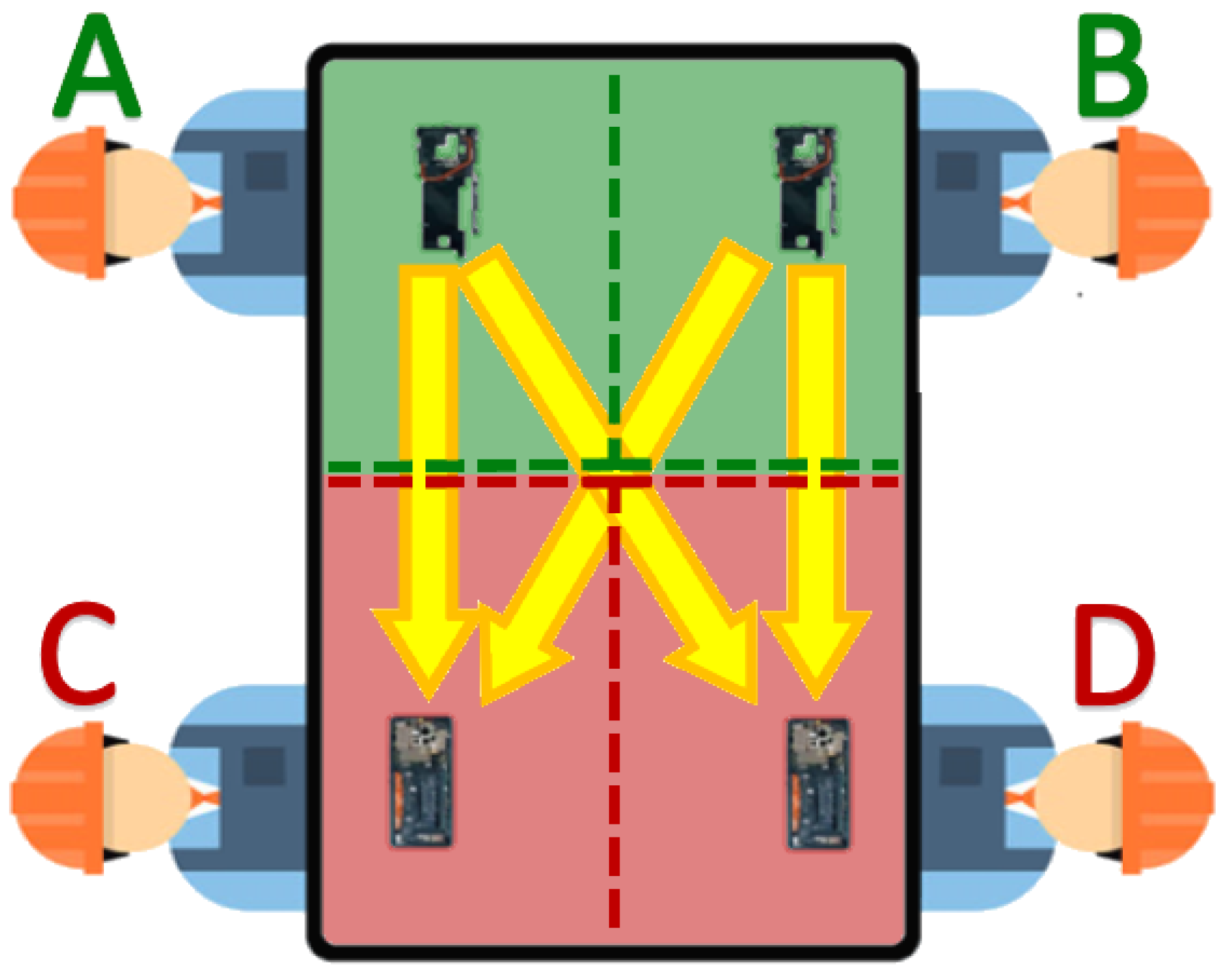
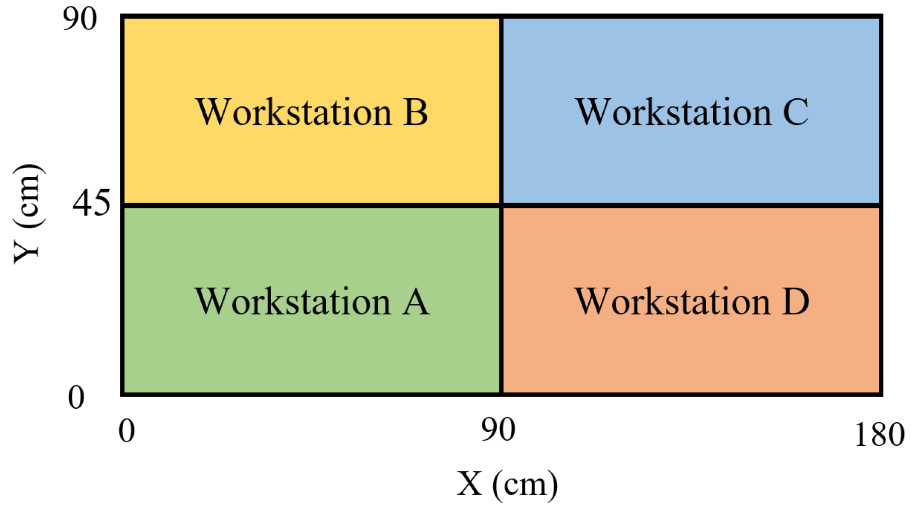
Figure 1. To this aim, the proposed system should keep track of the workstations where the objects were assembled and for how long. For this reason, in this section, we carry out a further set of experiments in which we evaluate the performance of the three chosen models in a scenario that emulates the specific one considered in this work. To this aim, we divided the workspace into four workstations labeled A, B, C, and D, as shown in
Figure 22. The size of the workstations was fixed at 90 × 45 cm.
In order to evaluate the three selected models, all datasets presented in
Section 4.3 are used. The data are divided randomly as 70% for training and 30% for testing, thus resulting in two new datasets, i.e., DTest and DTrain, with 15,000 and 6430 values, respectively. The three models (KNND, Liu_k, and RNN_k) are trained with DTrain without any pre-information or data from the previous experiments (no pre-training). The trained models are tested with DTrain and the results are reported in
Table 5. As we can see, the three models result in different performances: the KNND achieves an accuracy of 99% for the correct workstation recognition, and then we have the Liu_k model at 97% and RNN_k at 95%. These results show that these models can be used for workstation localization with very good performance and that the KNND achieves the best outcomes.
6. Conclusions
In this work, we assessed different methodologies for an assembly line localization system based on Bluetooth beacons. To this aim, a proof of concept implementation of a sensorized workbench is developed and used initially to create a realistic dataset. Using the collected data, different methodologies were trained based on regressors, CNNs and RNNs, respectively. The implementation of the proposed localization system in an industrial environment presents challenges that are sometimes difficult to recreate in the laboratory, such as signal interference, beacon maintenance, scalability, and human error. Signal interference can compromise tracking accuracy, while beacon maintenance and scalability require careful planning. Human error is another aspect that is difficult to take into account because there are many different cases to exploit, such as a worker breaking a BLE tag. Ensuring location accuracy and adaptability to environmental changes is crucial, as is the training of workers. With our study, we tried to address these challenges in a systematic way, also taking these issues into consideration Our experiments highlighted that KNND, in particular, can offer a very good localization accuracy in the industrial production monitoring use case, which can reach up to 99%, thus showing the possibility of implementing a short-range localization system with good accuracy. In future work, we plan to extend the proposed positioning system in order to track movements, as at the moment, only the static location of objects is supported.


 ,
, 


