FOCUSeR: A Fog Online Context-Aware Up-to-Date Sensor Ranking Method

Abstract

Data obtained from sensors connected to wireless sensor networks must be stored and processed to enable environments such as smart cities. However, with the exponential growth in the number of devices at the edge of the network, it is necessary to implement robust techniques, capable of selecting reliable data sources and meeting low latency requirements, in order to serve critical applications. Thus, to overcome these challenges, this research work presents FOCUSeR, a method for ranking sensors. The method uses the evaluation of data as a criterion for the ranking, allowing us to identify occurrences of failures in sensors and anomalies in environments. In order to meet the requirements inherent to WSNs, the proposed method was developed to run in a fog computing environment, using online learning and constant updating over time to avoid effects such as time drift. The generated ranking lists are managed through distributed hash tables. To provide reliability to the experimental results, a real experimental environment was developed. Moreover, using this developed testbed, a dataset with labels was created, to support the evaluation of the method. In addition, four other real datasets were used, three of which were labeled through artificial fault injection. These datasets were labeled in a related work that focused on injecting artificial faults. The experimental results obtained demonstrate that the proposed approach can provide reliability in the use of sensor data, using low computational resources and reducing latency in the sensor selection process. Precision rates are approximately 98% and Accuracy rates are greater than 94% across all datasets. In addition, the analyses carried out show that the Accuracy has an increasing rate as the number of samples also increases. Results obtained in the failure data recovery also demonstrate the feasibility of the proposal in this resource.

1. Introduction

Advances in low-cost sensor manufacturing and the miniaturization of microelectronic systems are the main factors responsible for the development of sensing, computing, and communication technologies, represented by smart sensors [1]. Smart sensor nodes are low-power devices equipped with a power supply, typically a battery, a processor, memory, a radio, and at least one sensor. Eventually, actuators can be incorporated to allow adjustments in sensor parameters, and sensor the movement or even monitoring of available energy. As sensors are usually deployed in difficult-to-access places, communication needs to be done through wireless devices, such as radios, responsible for transferring data to an access point in a fixed infrastructure [2].

These sensor nodes collect information about the surrounding environment and transmit this data to the Internet. The demand for environmental monitoring, which, through the control of critical values, avoids failures and minimizes the impact of extreme events caused by climate change or human interventions, has leveraged the development of wireless sensor networks (WSNs). The development of WSNs began around the 1980s, but it was only in 2001 that they really became the focus of research and industry interest [3]. Typically, a WSN consists of several sensor nodes (a few tens to thousands) working together to monitor a region for data about the environment and has little or no infrastructure. Unlike traditional networks, a WSN typically has resource constraints that include a limited amount of power, short communication range, low bandwidth, and limited processing and storage on each node. Design constraints depend on the application and are based on the monitored environment [2,4]. In the case of IoT, developed in parallel with WSNs [5], a specific communication technology is not assumed [3].

WSNs are great sources of big data generation due to the large number of nodes connected to the network. In these networks, large-scale data collected by sensors can be distributed, processed and used by various services and applications. However, as the number of objects added to the IoT is approaching 200 billion, and the number of sensors is already over 50 billion [6], the data generated far exceeds the capabilities of existing IT architectures and infrastructures. In scenarios where the real-time requirement is present, the available computing power needs to be even more robust.

The cloud computing model is a great alternative for managing these large volumes of data, providing greater processing capacity without affecting performance. However, when it comes to latency-sensitive applications, these characteristics may not be sufficient to meet services where delay requirements are present [7]. This type of service requires the network nodes to be close to the end-user, so that the time between the request and the response is as short as possible [8].

To overcome these obstacles, CISCO Systems, a company specialized in equipment and services for telecommunications, proposed the creation of the fog computing platform [8]. Fog computing is a horizontal, physical, or virtual resource paradigm that resides between smart end devices and the cloud or traditional data centers. This paradigm supports latency-sensitive applications by providing scalable, distributed compute, storage, and network connectivity [9]. In this architecture, each smart sensor node is connected to a fog computing device. These devices can be interconnected and are linked to the cloud [10]. By allowing the use of data produced by sensors, this architecture adds intelligence to environments. This is made possible by accessing necessary information related to environments, by collecting and analyzing past and present data. Thus, these data will support optimal decision-making about people and their environments, preferably in real time [8].

Edge computing (EC), on the other hand, is a paradigm in which communication, computing, control and storage resources are placed at the edge of the Internet, close to mobile devices, sensors, actuators, connected things and end users [11]. Applications running on EC will perform actions locally before connecting to the cloud. However, the actions that can be performed are limited by the modest computational resources characteristic of the devices in this layer of the network.

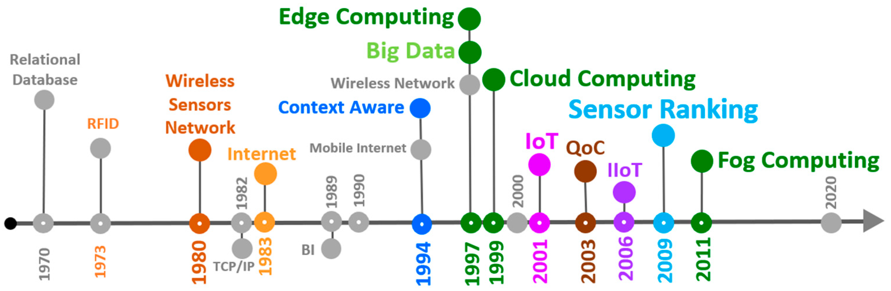
The timeline shown in Figure 1 presents these various technologies, which are related to the growth in the volume of data produced by sensors, as well as the technologies that have emerged to meet the demands of services and applications. Analyzing the image, it is possible to verify that there is a trend towards the miniaturization of the devices and that data analysis and processing has moved toward these devices.

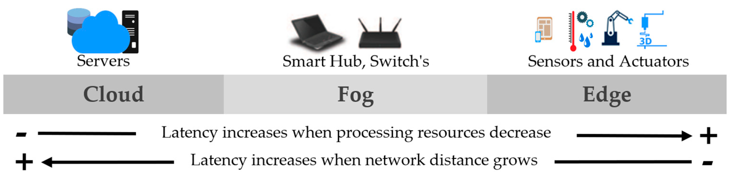
It can be said that latency in data transmission is one of the main factors that boosted this development. As can be seen in Figure 2, there are two factors that directly affect latency: the network distance and the power of the processing devices. In this way, to further reduce latency in the use of the service, data processing is performed in the Fog Computing layer of the network. This provides data processing, analysis and storage close to endpoints, allowing tools to be deployed outside of the cloud. It also favors the use of high-performance applications capable of processing and storing data close to where it is generated, allowing for very low latency and intelligent, real-time responsiveness [12,13].

In addition, when processing sensor data, it is necessary to understand the context in which the data was captured, requiring processes to become intelligent. Thus, understanding the context, or the situation in which the capture takes place, using sensor data and then acting autonomously, requires detection and learning. This is called context-aware computing. Quality of context (QoC) provides a set of metrics with information that helps in resolving conflicts related to contextual information [14].

To allow the use of these techniques in the processing of this large volume of data produced by sensors, IoT middleware solutions have been adopted [15,16]. An IoT middleware is used to manage sensor data allowing its use by different applications, thus acting as an interface between the user/application and the sensor networks and allowing for an abstraction of the heterogeneity inherent in sensor data sources [1].

An IoT middleware offers capabilities for acquiring, discovering, indexing, ranking and querying sensors and data related to these sensors [1,17]. Indexing consists of storing and indexing data about sensors, to speed up the process of selecting a subset of sensors. Sensor ranking is performed by prioritizing criteria such as data quality, device availability, energy efficiency and network latency. This task can be performed based on the data generated by the sensor (content) and on the available information about the conditions under which these data were generated (context). Applications such as industry and healthcare that require reliability associated with processing and providing data with low latency are examples of usage scenarios [18].

The relevance of the proposed approach is related to the ability to provide a quick way, and with a high degree of reliability, to select data sources (sensors), for decision making and control of environments and devices, in addition to carrying out these activities of distributed form to ensure scalability, an essential requirement in the IoT environment [11]. The exponential growth in the number of sensors in the IoT environment justifies the need for this type of activity.

Considering these premises, this paper presents the result of a research work in which we propose a method for ranking sensors. The proposed method is based on the fact that solutions for sensor ranking must be feasible considering the heterogeneity, low computational capacity and high volume of connected devices. Furthermore, it considers that the real-time requirement is present in several services that make use of sensor data.

The rest of the paper is organized as follows. Section 2 presents the concepts involved, as well as describes the proposed method and the related works. Section 3 describes the experimental environment develop and the experimental results. In Section 4, the results obtained are discussed, and in Section 5, the Conclusions and Future Works are presented.

2. Background

This section describes the basic concepts related to the applied techniques and algorithms. The main concepts described are related to the interquartile range, used in the first evaluation of the data, as well as those related to the matrix profile method, used in the second evaluation of the data, to identify anomalous segments in time series. The theory of quality of context (QoC), from which some parameters are used, and the definition of distributed hash tables (DHT), which are used to manage distributed ranking lists, are also presented. After presenting these concepts, the proposed method is described in detail.

2.1. Active Perception Theory

Active perception can be defined as a problem of an intelligent data acquisition process. This process must define and measure environmental parameters and errors, which, in turn, can be fed back to control the data acquisition process. The importance of this process is that time is not spent processing and improving imperfect data, but rather accepting imperfect and noisy data as a matter of fact and incorporating it into the overall processing strategy [19]. Thus, perception is not a passive process, but an active one. Perceptions do not merely fall on sensors as rain falls on the ground. During the act of looking, the pupils adjust to the level of illumination, the eyes bring the world into sharp focus, converge or diverge, the heads move to improve the vision of something [19]. This adaptability is crucial for survival in an uncertain world. Thus, the problem of active perception can be defined as the use of control strategies applied to the data acquisition process, which, in turn, will depend on the interpretation of the data and the objective of the task [19].

Whereas perception depends on context, other senses and time, active perception has four levels: sensation, perception, perception over time and active perception. Sensation involves the process of capturing the data. After capture, perception interprets and gives meaning to this data. By observing a process over a period of time, it is possible to improve the interpretation of this data. This process is called perception over time, indicating that it is possible to evaluate perception in relation to another perception. The last level is active perception, which includes reasoning, decision and actions based on the information received [20,21,22].

2.2. Interquartile Range

The interquartile range (IQR) metric is useful to indicate whether the values of a dataset can be considered outliers [23]. Quartiles are the separators that divide a numerical dataset into four equal parts. The first quartile (Q1) is the value of the set that delimits the 25% smaller values. The second quartile (Q2) is the median itself. The third quartile (Q3) is the value that delimits the 25% higher values. Thus, the first range of data starts at the smallest value and goes to Q1. The second range, between 25% and 50% are values greater than Q1 and less than Q2, and so on [24]. The interquartile range is the difference between Q3 and Q1. The intention is to create thresholds using the value of the IQR index to allow the identification of values that are far from the frequent values of the data set.

2.3. t-Digest

When dealing with time series, many interesting statistics are difficult to calculate. For example, to find the most common value, or the number of distinct values, or even just the median without sorting all the data, the most popular approach is to calculate a small summary of the data (called a digest or a sketch), and then use that summary to estimate the desired value, such as a median or a quartile. The t-digest provides these statistics with an order-of-magnitude better accuracy than other existing algorithms, and with very low computational complexity [25].

2.4. Fault/Outlier Model

Failures in capturing and transmitting data, obtained from sensors, normally occur in one capture and are normalized in the next (outlier point). The reason is that the disturbances related to these problems are mostly transient, caused by imbalances that lead to momentary instabilities [26]. Thus, when interference occurs in a single measurement, generating a single incorrect value, there is a high probability that these data will be misinterpreted. This kind of problem can be mitigated by analyzing time slices of data (subsequences).

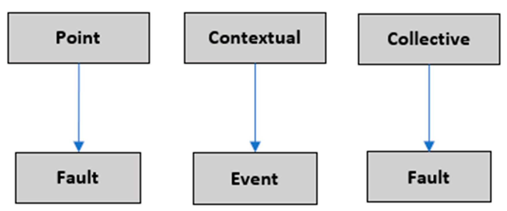
In this work, the values are first analyzed individually, and they are then evaluated using comparisons between subsequences of data. Values that are far from frequent values are considered failures, and the rest of the data are considered events. In the case of a point outlier, this evaluation is simple. When considering subsequences of data, if any value of the subsequence is discrepant from the rest of the data, the subsequence is interpreted as a failure (collective outlier), otherwise, as an event (contextual outlier). The taxonomy presented in Figure 3 describes this method.

When a failure occurs, the proposal also delivers, along with the other output variables, a classification for the type of outlier, based on the information presented in the failure/outlier model and in the scheme presented in

Table 1. Output fault/outlier type (cell background colors help identify outlier types).

		First Level
	Output Label	Normal	Anomaly	Failure
Second Level	Normal	Normal	Point Failure	Point Failure
	Anomaly	Context Event	Context Event	Context Event
	Failure	Collective Failure	Collective Failure	Collective Failure

.

The criteria adopted for the decision consider that faults identified at the first level, that is, in the individual analysis of the sample, are highly likely to represent transient faults in the sensor. Thus, when only the first level fails, the error is considered a point failure. At the second level, in the analysis of a subsequence of data, when an anomaly is identified, the data are considered as a context event and not as a failure. If a fault is also identified at the first level, the data are considered a collective failure. Figure 4 presents an example of these types of outliers.

In this proposal, the data generated by sensors are classified with as normal, anomaly (event), and failure. Data considered as normal are those that indicate that both the sensor and the environment in which the measurement is being made are stable (no anomalies) and the reading process was not affected by interference during data capture and transmission. Data in this range of values represent the data most frequently generated by the sensor.

When a measurement affected by a fault is analyzed as a time series (slice), the subsequence corresponding to that fault will be different from the normal trend of the entire time series. However, this will only be true if the deviation from normality is large enough to influence the measurement of the entire segment, which occurs in persistent failures. In the case of transient failures, a single abnormal data point, the influence on series measurement is less significant. Thus, when analyzed in a data segment, the disturbance caused is mitigated due to the presence of several other normal values.

In this second evaluation, the data can also be considered an anomaly, indicating the occurrence of anomalies in the environment. This occurs when several of the values in the data segment are relatively far from the normal range, but within a range of values that may exist in the environment’s domain (contextual outlier). This kind of data do not occur that often.

Finally, data considered as a failure are data that occur due to persistent failures in devices, affecting the capture or transmission of data (collective outlier). In this case, the range of values is further away from the other values, extrapolating the limits of valid values in the domain.

$$\left(Q1-FF\times IQR\right)\langle fi\rangle (Q3+FF\times IQR)$$

(1)

$$\left(Q1-AF\times IQR\right)<ai<\left(Q3+AF\times IQR\right)$$

(2)

The IQR metric is applied to obtain the indicators to be used in the evaluation of the data. In the case of evaluating single data samples, the IQR is applied to a data set of values produced by the sensors. In the case of evaluating data subsequences, the IQR is applied to the distance profile generated by the matrix profile algorithm.

Equations (1) and (2) use the anomaly index (ai) and failure index (fi) to label samples. Equation (1) is used to verify if a value is considered a failure and Equation (2) for values considered anomalies. The anomaly factor (AF) was set to 3 (three) and failure factor (FF) to AF × 2. Normally, when calculating the cut of outliers using the IQR metric, a K coefficient usually equal to 1.5 (one point five) is adopted [27]. In preliminary studies carried out in the development of the proposed method, this coefficient proved to be inefficient as a threshold to define anomalies and failures related to the approach of this work.

Figure 5 shows an example of application of this metric: the samples located between the green lines represent the data considered normal; the samples between the green and red lines represent anomalous data, and the points above the red line represent probable failure data.

2.5. Matrix Profile

Here, the scalable matrix profile algorithm [28] and some of its variations relevant to this work, will be described. The algorithm is used in the proposal to create time series subsequence joins. The algorithm is simple, fast, parallelizable, and parameter free, and can be incrementally updated. As will be shown, the algorithm is extremely efficient for discord discovery tasks.

The following definitions and notations were taken from [28]. A time series T is a finite sequence of samples T = [t₁, t₂, …, t_n], taken at increasing instants of time, of length n. A subsequence is a small continuous subsets T_i,m obtained from T, of length m, starting in i. T_i,m = [t_i, t_i+1,…, t_i+m−1], where 1 ≤ i ≤ n − m + 1. A subsequence refers to a sequence of time series samples ordered in time.

The Euclidean distance metric is used to produce the similarity measure between subsequences t₁ and t₂, with m samples in each subsequence. A zero distance, that is, maximum similarity, occurs only when two segments are very similar in all n samples. The Euclidean metric is presented in Equation (3).

$$d\left(t_1, t_2\right)=\sqrt{{\sum }_{i=1}^m{\left(t_1-t_2\right)}^2}$$

(3)

A distance profile D is a vector of the Euclidean distances between a given query and each subsequence in an all-subsequences set. When the query and all-subsequences set belong to the same time series, the distance profile must be zero at the query location, and close to zero before and just after [28]. An all-subsequences set A of a time series T is an ordered set of all possible subsequences of T obtained by sliding a window of length m across T:A = {T_1,m, T_2,m, …, T_n−m+1,m}, where m is a user-defined subsequence length. A[i] is used to denote T_i,m [28].

Given two all-subsequences sets A and B and two subsequences A[i] and B[j], a 1NN-join function θ1nn (A[i], B[j]) is a boolean function which returns “true” only if B[j] is the nearest neighbor of A[i] in the set B.

Given all-subsequences sets A and B, a similarity join set J_AB of A and B is a set containing pairs of each subsequence in A with its nearest neighbor in B:J_AB = {〈A[i], B[j]〉 | θ1nn(A[i], B[j])}. This is formally denoted as J_AB = A⋈ _θ1nnB.

A matrix profile P_AB is a vector of the Euclidean distances between each pair in J_AB. This vector is called the matrix profile because one way to compute it would be to compute the full distance matrix of all the subsequences in one time series with all the subsequence in another time series and extract the smallest value in each row (the smallest non-diagonal value for the self-join case). The profile has a host of interesting and exploitable properties. For example, the highest point on the profile corresponds to the time series discord (subsequences that are maximally different to all the rest) [28], the lowest points correspond to the locations of the best time series motif pair [29], that is, pairs of time series subsequences that are very similar to each other, and the variance can be seen as a measure of T’s complexity. Moreover, the histogram of the values in the matrix profile is the answer to the time series density estimation [30]. This special case of the similarity join set is named as self-similarity join set. Each element in the matrix profile tells us the Euclidean distance to the nearest neighbor, however, it does not tell us where that neighbor is located. This information is recorded in matrix profile index, a vector of integers that allows efficiently retrieve the nearest neighbor of an element by accessing the position indicated by each integer, that is, a I_AB of a similarity join set J_AB is a vector of integers where I_AB[i] = j if {A[i], B[j]} ∈ J_AB.

Mueen’s ultra-fast algorithm for similarity search (MASS) is a Euclidean distance similarity search algorithm for time series data that finds the nearest neighbor to a query and, unlike the dozens of time series KNN search algorithms in the literature [31], this algorithm calculates the distance to every subsequence, i.e., the distance profile of time series T. The algorithm uses an fast similarity search algorithm under Euclidean distance as a subroutine, exploiting the overlap between subsequences using the classic Fast Fourier Transform (FFT) algorithm to calculate the dot products between the query and all subsequences of the time series [28]. The algorithm produces one full row of the all-pair similarity matrix. The scalable time series anytime matrix profile (STAMP) [28] algorithm is a loop that computes each full row of the all-pair similarity matrix and updates the current “best-so-far” matrix profile when needed.

The STAMP is the batch version of the algorithm. Batch means that the algorithm needs to see the entire time series T_A and T_B (or just T_A if self-similarity join matrix profile is being calculated) before creating the matrix profile. But in the case of this research work, the interest is in building the matrix profile incrementally. Once the matrix profile has already been built in a batch approach, when new data arrives, an incremental adjustment of the current profile is performed. This algorithm is called STAMPI (STAMP incremental) algorithm.

2.6. Evaluation Measures

The evaluation metrics commonly used to measure the effectiveness of anomaly detection performance present in related works are Accuracy, Precision, Recall, and F1 score, as presented in Equations (4)–(7) respectively. In these Equations, TP = true positive, TN = true negative, FP = false positive, and FN = false negative. The results are presented as a percentage.

$$Accuracy=\frac{TP+TN}{TP+TN+FP+FN}$$

(4)

$$Precision=\frac{TP}{TP+FP}$$

(5)

$$Recall=\frac{TP}{TP+FN}$$

(6)

$$F1 Score=2\times \frac{Recall\times Precision}{Recall+Precision}$$

(7)

2.7. Distributed Hash Tables

Distributed hash tables (DHT) are excellent solutions for managing distributed lists. This method has a high degree of scalability and flexible support for query and update operations. DHT has a decentralized approach that provides fast mechanisms for storage, queries and updates. Are built on overlay networks in which network objects are spread out and identified with unique keys [32].

The Apache Cassandra tool implements a chord class algorithm [33]. Cassandra achieves horizontal scalability by partitioning all data stored on the system using a hash function called a consistent hash that is similar to a Chord model [34], and the Chord model in turn is based on DHT. This model provides a scalable and efficient protocol for dynamic research in P2P systems with frequent node inputs and outputs. It also provides mechanisms to facilitate resource finding, new node entries, and fault management. To improve scalability, the Chord node does not need routing information about all other nodes, but only a number of O (log N) nodes, and therefore the search needs a maximum of O (log N) messages.

3. Related Works

In this section, the most relevant works related to the ranking of sensors are presented.

The IoTCrowler [35] is a framework developed for the task of search IoT. The framework is composed of two layers: the crawling and processing layer that is responsible for constantly integrating new data sources into the framework; and the search and orchestration layer that contains components for handling search and subscription requests coming from IoT applications or users. In the crawling and processing layer, the data stream is monitored to allow fault detection as well as fault recovery. Here, the search indexes are also generated. In the search and orchestration layer, the orchestrator is the entry point for any user or application that wants to search for IoT devices. This layer can provide an endpoint to receive notifications about faults. In this layer, the ranking component uses the built indices, given constraints, and enriched information to rank the found data sources before they are sent back to the user or application.

Bharti proposed the VoI-based sensor ranking mechanism VoISRAM [36], which is primarily intended to exploit the classification engine’s gateway services to strike a balance between application-specific QoS requirements and network power consumption. The method proposed an information-based value-based sensor service ranking mechanism that models the classification of a sensor service as an information attribute value while considering its context of use in the corresponding application. In [37] the GaaS, a cross-platform gateway architecture for retrieving the sensory data from the low-power IoT sensors is proposed. The architecture leverages multithreading to enable the gateway from simultaneously connecting to several IoT sensors. To regulate the Bluetooth low energy connections, the work devised two distinct priority-based schedulers which rank the IoT sensors, before generating the connection schedule.

In the work of Nesa and Banerjee [38], a dynamic sensor activation algorithm, inspired by the PageRank algorithm, called SensorRank, is proposed. Unlike the PageRank algorithm, which requires only external links to classify web pages, SensorRank dynamically analyzes the network topology in terms of relative distances, link qualities, and the remaining power of the devices, based on which the sensors are classified. Dautov and Distefano [39] present a decentralized architecture to group heterogeneous devices and execute data-intensive IoT workflows at the edge of the network. The proposed approach initially divides a complex workflow into more straightforward tasks, then discovers and selects suitable edge devices and, finally, allocates tasks to the selected nodes, connecting them to recompose the original workflow. The discovery and selection of suitable edge devices are made based on functional and non-functional task requirements, respectively, before mapping the decomposed tasks to the selected nodes. The ranking of devices is calculated at the device selection stage using non-functional requirements. In the work of Ruta et al. [40], the ranking of the devices is based on a metric that calculates the semantic distance between the user’s requirements and the semantic description of each device. In the work by Kertiou et al. [18], the authors use context information from sensors with a dynamic skyline operator to reduce the search space and select the best sensors according to user requirements. In Kang et al. [41], the frequency at which users use individual items, the distances between users and devices (services), the network’s QoS, the device’s performance and its history of operations, and the priority set by the user are used to calculate the device’s ranking information.

In the work of Yuen et al. [42], the primitive cognitive network process (P-CNP) method is used to derive the importance of sensor nodes based on two types of QoS parameters: network-based (latency, bandwidth, and throughput) and based on the sensor (accuracy, reliability, and cost). The parameters receive weights according to their importance to the user. The ranking of the sensor is generated using the values of the attributes and weights.

The work of Perera et al. [43] presents an architecture for providing scalability, as well as a research tool, in which it establishes two classes of user parameters (negotiable and non-negotiable). For example, if a user wants to measure the temperature in a given location, the result (the list of sensors) must contain only sensors to measure the temperature. To index and order the sensors, user preferences are used with an indexing technique using the weighted Euclidean distance metric called the Comparative Priority Based Weighted Index (CPWI). In the paper by Truong, Römer, and Chen [44], a proposal for researching similarity sensors is presented. In the proposal, a user provides a sensor and a fraction of its past output as an example and requests sensors that have produced similar output in the past. Regarding the time factor, the proposal uses a time series to search for sensors when comparisons are made by similarity. A comparison of the sensors is made using fuzzy logic to compare each of the candidate sensors with the sensor provided by the user. The result of the similarity metric is used to build the sensor ranking.

Elahi et al. [45] were the first to use the term ranking of sensors. The work focuses on using data produced by sensors centered on people, considering that habits can indicate future behavior, and thus use the data generated by these sensors to create forecasting models. This process calculates, for each sensor, an estimate of the probability that corresponds to the query and the sensors in decreasing order of probability. The effort is spent first on sensors with a high probability of corresponding to the query. This approach, in addition to not meeting situations in which low latency requirements are present, as it is very specific, needs to develop (train) a forecasting model for each dataset, making the intervention of a specialist mandatory and requiring a long preparation time for use. Another negative aspect is that the ranking calculation is performed after receiving the user’s parameters, which increases the process latency. In addition to the characteristics described, the proposal cannot be executed in a distributed manner, which poses an obstacle when considering the need for scalability of a solution aimed at the IoT network.

Table 2. Related works.

Work		Features Characteristics
	Distributed	Fog/Edge Tier	Low Complexity	Ready Ranking List	Data Evaluation	Fault/Outlier Type	Online	Up to Date	Replace Failure Data	Real Testbed	Real Datasets
FOCUSeR	√	√	√	√	√	√	√	√	√	√	√
Mekala (2021)	√	√	-	-	√	-	-	-	-	-	-
Iggena (2021)	√	-	√	-	√	√	-	-	√	-	√
Costa (2021)	-	√	√	√	√	-	-	-	-	-	√
Bharti (2021)	√	√	√	√	-	-	-	-	-	-	-
Liu (2020)	-	-	-	-	-	-	-	-	-	-	√
Lee (2020)	-	-	√	-	-	-	-	-	-	-	-
Sundar (2019)	-	-	-	-	-	-	-	-	-	-	-
Biró (2019)	-	-	√	-	-	-	-	-	-	-	-
Abdelaal (2019)	-	√	√	-	-	-	-	-	-	√	√
Costa (2019)	-	√	√	√	√	-	-	-	-	-	√
Nesa (2019)	√	-	-	√	-	-	-	-	√	-	√
Dautov (2019)	√	-	-	√	-	-	-	-	-	√	√
Ruta (2019)	√	√	√	-	√	√	-	-	-	√	√
Kakunsi (2018)	-	-	√	-	-	-	-	-	-	-	-
Kertiou (2018)	√	-	√	-	-	-	-	-	-	√	√
Dilli (2018)	-	-	√	√	-	-	-	-	-	-	-
Hussain (2018)	-	-	√	√	-	-	-	-	-	-	-
Nunes (2018)	-	-	√	-	-	-	-	-	-	-	√
Kang (2016)	√	√	√	√	-	-	-	-	-	-	-
Zhang (2016)	√	-	-	-	-	-	-	-	-	-	√
Neha (2016)	-	-	√	-	-	-	-	-	-	-	-
Wang (2015)	√	-	√	-	-	-	-	-	-	-	-
Yuen (2014)	-	-	√	-	√	√	-	-	-	-	-
Cabral (2014)	√	-	√	√	-	-	-	-	-	-	√
Niu (2014)	-	-	-	-	-	-	-	-	-	-	-
Perera (2014)	√	-	√	√	-	-	-	-	-	-	√
Truong (2012)	√	-	√	√	-	-	-	-	-	√	√
Walters (2011)	√	√	√	-	-	-	-	-	-	-	-
Wang (2010)	√	-	√	√	-	-	-	-	-	√	-
Ostermaier (2010)	√	-	√	-	-	-	-	-	-	√	√
Elahi (2009)	√	√	-	√	-	-	-	-	-	-	√

presents a list of works related to this proposal. The symbology of the table uses a dash if the work does not meet the presented resource and a special sign if it does. The features refer, in this order, to: whether the proposal is capable of running totally in a distributed network environment; in which computing layer (cloud, fog, or edge) the algorithm runs; if the algorithm has low computational complexity; if the ranking list is always ready (no need to generate it for each query); if the work considers the evaluation of the data generated by the sensor; if the proposal seeks to identify and differentiate faults and anomalies; whether the data assessment process requires training; whether the data assessment process is kept up to date; whether the proposal makes use of data recovery from other sensors when failures occur in the current sensor; whether the experimental environment used in the evaluation of the proposal is close to a real processing environment; and finally, whether real data were used in the evaluation of the proposal.

According to the bibliographic research carried out, it is possible to verify that few works address the evaluation of data, and among these, none of the proposals use online training or keep up to date over time. Many other works address the issue of fault detection, but as they do not propose to offer solutions for sensor ranking, they were not considered in this discussion [46,47].

FOCUSeR Contributions

From the analysis of related works, it is possible to assume that a reasonable ranking method must satisfy several requirements [35,48], in order to provide a service that meets the quality of service when used in a real scenario.

The related works analyzed present different approaches for generating sensor ranking lists, demonstrating the importance of the activity for the correct use of IoT data. However, despite the related proposals showing promising results, it is possible to note some challenges and issues that still need to be overcome. Thus, when considering these problems, it is possible to list a set of requirements that must be met in the sensor ranking processes. These requirements are listed below:

• Requirement 1 (R1): the ranking list should be distributed in a distributed way.
• Requirement 2 (R2): to reduce latency in end-user queries and applications where real-time requirements are present, it is desirable that the ranking service runs close to the data source, that is, in the Edge or Fog Computing layers.
• Requirement 3 (R3): to be viable in terms of processing, and considering R2, it is essential that the algorithm has low time complexity.
• Requirement 4 (R4): with the same purpose as R2, the ranking list must always be ready, to prevent the user from having to wait for the list to be generated on each request.
• Requirement 5 (R5): one of the main challenges of a WSN is how to efficiently deliver the detected measurements to the destination with maximum fidelity to the probed data. For this, data measured by sensors require an efficient classification measure to differentiate between normal and anomalous values [49]. Thus, not performing data evaluation can compromise the performance of WSNs and the services and applications interested in that data.
• Requirement 6 (R6): considering that WSN is highly dynamic, distributed, heterogeneous and with a large number of objects, using data evaluation (R5) with methods that require training becomes unfeasible. Thus, it is essential that ranking algorithms have online learning.
• Requirement 7 (R7): since the objects in the WSNs are dynamic, and in order to avoid effects such as “concept drift”, it is important to use methods capable of avoiding the lag of the models.
• Requirement 8 (R8): verifying the viability of the algorithm, carrying out the tests in environments as close as possible to real processing environments, corroborates the results of the work.
• Requirement 9 (R9): here the intention is similar to that presented in R8.

Thus, after presenting the requirements considered important for a sensor ranking method, we present the contributions of this research work:

• Run in a distributed environment (R1).
• The method is able to meet the real-time requirements using low computational resources and thus providing low latency in queries (R2, R3 and R4).
• Provides a method capable of delivering, together with the data obtained from the sensors, metadata with information about the quality, reliability and nature of this data and the sensor itself (R5, R6 and R7).
• The proposed method is free of training and keeps up to date over time (R6 and R7).
• Evaluate experimental results with real data and in real environments (R8 and R9).
• The proposed method is capable of recomposing failure data by searching for sensors, capable of providing the same information, in the surrounding locations.

4. Fog Online Context-Aware Up-to-Date Sensor Ranking (FOCUSeR) Method

This section describes the proposed method FOCUSeR and some important approaches used in the proposal.

4.1. Sensor Ranking Inspired on Active Perception Theory

The ranking method proposed in this work is inspired by the theory of active perception. Similarly, in this proposal, the task of ranking sensors is performed through an analysis that allows for different levels of reasoning according to the context found. In addition, it is characterized as active because it is able to find alternatives to the problems encountered (failures and anomalies) by seeking reliable data sources.

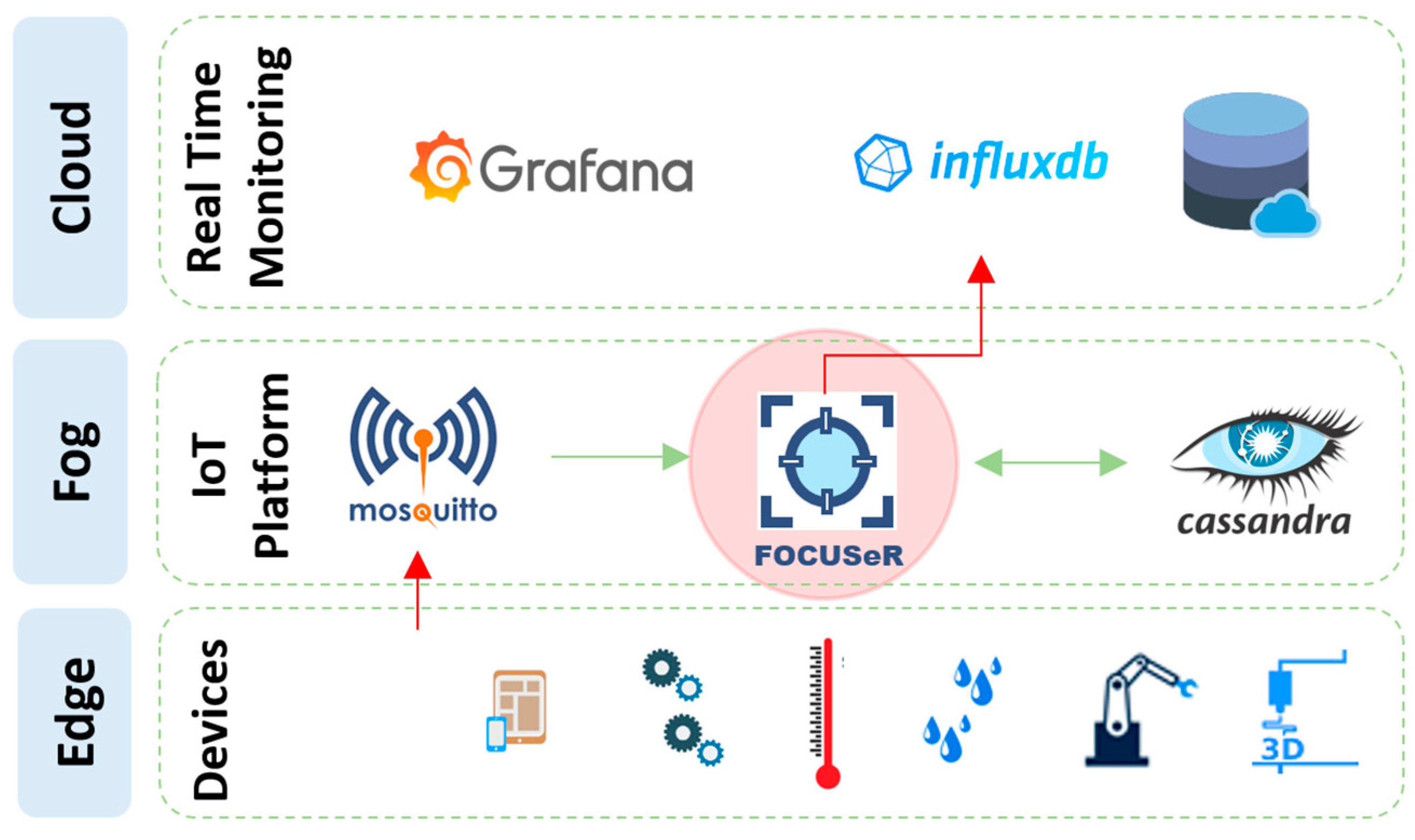
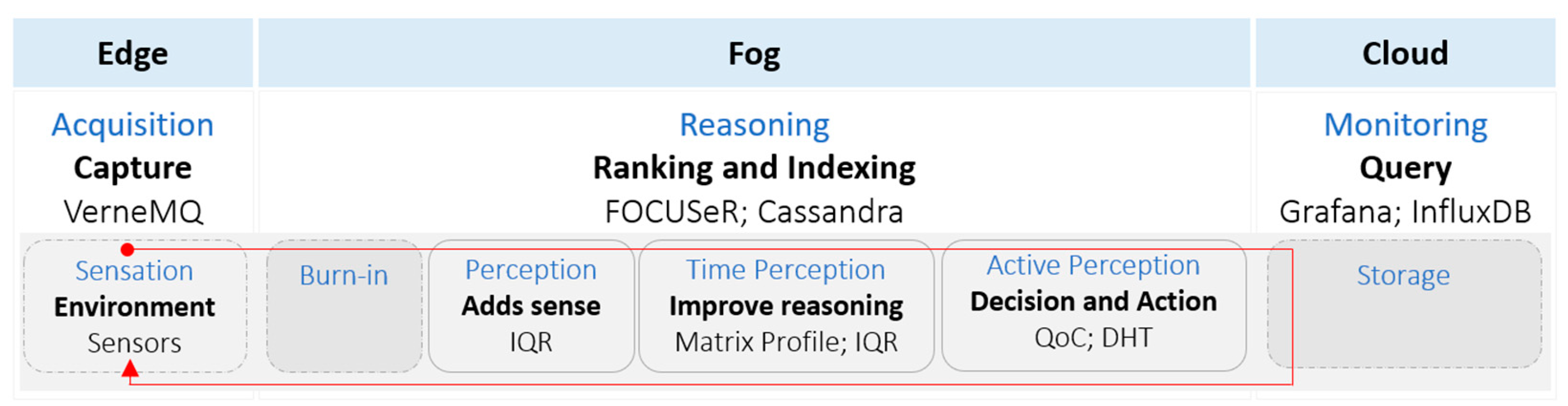
Figure 6 shows an overview of all steps involved in this proposal. At the top of the figure, the network layers (Edge, Fog, and Cloud) are first identified. Below the network layers, are presented (from left to right): the acquisition, reasoning and monitoring levels; the standard functions (bold text), commonly found in middleware’s for sensor ranking; and the tools used to perform each function in the experimental environment developed to evaluate the proposal.

The boxes in the lower part of the figure presents the levels of the ranking process, detailing the flow of information in the proposal. This part of the figure presents the levels of active perception (boxes with light gray background color), starting with the sensation activity, that is, collecting data in the environment and following the direction of the red arrow, perception, perception over time and active perception. In this flow, the burn-in and storage activities (boxes with a darker gray background color) of the data produced by the proposal are also presented.

The first level of active perception, sensation, is performed by the sensors and represents the capture of data produced by them. So, the burn-in activity is the one in which the indicators for using the IQR metric are created. After the burn-in stage, the next levels of active perception appear.

The flow ends with the data persistence activity, used to demonstrate monitoring examples. The red arrow in the image informs that the flow returns to the environment, indicating the execution of actions to be taken defined at the level of active perception. In the following subsections, the implementations of each level will be detailed.

4.2. Burn-In

Due to the heterogeneity of the environments monitored by sensors, it is impossible to manually adjust the parameters for each sensor. As a way to overcome this limitation, this proposal uses the online learning approach. In the burn-in step, the samples initially obtained from each sensor are used to generate the anomaly and failure indices presented in Equations (1) and (2). The number of samples initially used to generate the indices is an input parameter of the proposal’s algorithm. In the tests performed, the first 2000 (two thousand) samples were used, with the exception of the FOCUSeR and SmartSantander datasets in which the first 500 (five hundred) were used due to the low number of samples for each sensor. These values were chosen after a parameter sensitivity analysis, as will be described in the evaluation results section.

The update of the anomaly and failure index (Equations (1) and (2)), according to the value defined in the burn-in parameter, proved to be effective, which was verified through an increase in the Accuracy rates, as will be shown.

The t-digest data structure was used to allow updating these indexes without having to keep the entire dataset already seen in memory.

4.3. First Level

At the first level of proposal processing, that is, perception, the anomaly and failure indices are applied to the samples that arrive in the system. As a result of this evaluation, the data can be classified as normal, anomaly or failure.

4.4. Second Level

This level uses time to evaluate the data. The adoption of this approach allows to distinguish transient faults from persistent faults and also, by examining the data from the point of view of a data slice, it allows a better identification of the patterns contained in that dataset. If a measurement affected by a fault is analyzed as a time series, then the sequence of samples or segments corresponding to the fault will be distinct from the normal trend of the time series. In other words, this segment will be considered anomalous.

To implement this concept, the matrix profile algorithm was chosen. The algorithm is initially run with the burn-in sample data (batch). Once the distance profile is generated, the IQR metric is applied to generate the anomaly and failure indices for segments. After the burn-in stage, the matrix profile is updated with each new data and this data is evaluated using the generated indices, in order to identify the segments that diverge from the other segments of the data set (in this case, all segments known so far). In the same way as in the previous level, the segments are also classified in the normal, anomaly and failure categories.

4.5. Third Level

In the final level, according to the classifications obtained in the first two levels, the type of outlier is identified. The sensor index is also updated with the new information. To update the index, the data are processed using the concepts of Quality of Context (QoC) theory. The QoC parameters used in this work are described below.

The trustworthiness (T) parameter of QoC (Equation (8)) is used as an indicator in order to generate the ranking of sensors. In the trustworthiness parameter, the value 0 (zero) means that this context source is not reliable, and 1 (one) represents total reliability in the context source [50]. In Equation (8), the parameter T is the reliability, the ctx is the set of trusted context elements for a given sensor i and W is the total number of sensor context elements and must be greater than zero.

$$T_i=\frac{NumberOfRealiableSamples\left(ct{x}_i\right)}{W_i}$$

(8)

In the final level, that is, the active perception level, when a failure is identified in the sensor data, the active perception function is then activated, and “the vision is adjusted” to check if there is another sensor close enough to provide the measurement of the environment that can replace the measurement provided by the unreliable sensor. For this task, other QoC parameters are used.

The sensor_location [51] parameter, which describes the location of the sensor at the time the context information was collected, is used to enable the retrieve of similar sensors (with the same features) surrounding some sensor that is in abnormal state. To make this search quick and straightforward in the sensor list, geospatial data is previously stored in Apache Cassandra. By storing the data in this way, it is possible to find points close to a certain location. The challenge here is to find a key capable of restricting the potential list of locations and avoiding consulting many keys at once [52].

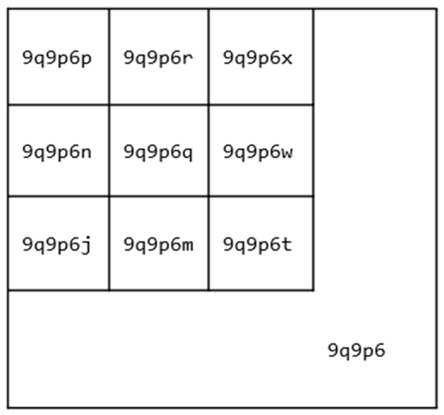
Although there is more than one possible data structure used for this purpose, geohashing was chosen because it offers several benefits over other techniques. A geohash is a base 32 representation of a geographic area, where each additional digit represents greater accuracy. The property of geohashes that makes them particularly suitable for geospatial research is that adding a level of precision to given geohash results in an area contained in the lower precision value [52]. An example can be seen in Figure 7, which shows a diagram with the geohash 9q9p6, containing a series of more precise geohashes contained within it. All the smaller geohashes begin with the 9q9p6 prefix.

After performing a search using the location data, the found data is evaluated with the QoC parameters described below. These parameters were used to verify the validity of context information over time, that is, to verify that the data did not expire according to the parameters.

$$Age\left(ct{x}_i\right)=t_{curr}-t_{meas}\left(ct{x}_i\right)$$

(9)

$$Timeliness\left(ct{x}_i\right)=\{\begin{array}{c}1-\frac{Age\left(ct{x}_i\right)}{TimePeriod\left(ct{x}_i\right)} : if Age\left(ct{x}_i\right)<TimePeriod\left(ct{x}_i\right)\\ 0 :otherwise \end{array}$$

(10)

Age of context object ctx_i (Equation (9)) is calculated by taking the difference between the current time, t_curr, and the measurement time of that context object ctx_i, t_meas(ctx_i). Information about the age of a context allows the consumer to assess its relevance in advance to process it. The Timeliness parameter (Equation (10)) is a measure that indicates the degree of freshness of a context object at a given time [51]. Newer information is often more relevant compared to older information. In most cases, old contexts can be discarded without significant consequences. The dynamic nature of this parameter is characteristic of real-time applications [53]. As the situation in pervasive environments changes very rapidly, applications using a context object without knowing the Timeliness of that context object may take undesired actions that can result in loss of resources. Timeliness of a context object can be measured objectively and subjectively. To obtain the subjective view of the timeliness of a context object, the validity time of the context object mentioned by the user is considered, regardless of the time period [51]. However, as this proposal does not consider the query parameters to generate the ranking, the value of 0.5 is assumed as the limit for the data age (Timeliness). The parameter TimePeriod indicates the time interval between two measurements. The value of Timeliness and the validity of context object decrease as the Age of that context object increases [51].

In addition to checking the freshness of the data produced, it is tested whether the value of the trustworthiness parameter is above 0.9, otherwise the sensor is considered unreliable. These parameters are configurable per dataset and do not influence ranking generation. They can be informed at the time of user queries.

The values set for the burn_in, window_size and iqr_refresh parameters are discussed in the results evaluation section.

The last step is to update the ranking of the sensors using the new values of the trustworthiness parameter as a key. The algorithm also feeds information regarding the last analyzed sample into the distributed hash tables, such as the classification of data into normal, anomaly and failure and a second category identifying the sample as normal, point outlier (failure), context outlier (anomaly) or collective outlier (failure). Algorithm 1 presents the entire process, whose abbreviations used are presented in

Table 3. List of abbreviations used in Algorithm 1.

Abbreviations	Definition
ptr	QoC parameter trustworthiness
ptl	QoC parameter timeliness
ptp	QoC parameter time_period
burn_in	Burn-in phase
pbin_sz	Number of samples to be used in the burn-in step
pw_sz	Size of the window to be used when comparing subsequences
piqr	Number of samples to be used to update IQR metric indicators
id	Sensor identification
val	Sensor measured value
lat	Sensor location latitude
lon	Sensor location longitude
dt	Sensor measurement capture date
tt	Updated QoC parameter trustworthiness
ft	Fault type
fsid	Identification of the sensor used in data recovery (nearby sensor)
fsv	Value captured by the nearby sensor
sl	Sample sliding window buffer
ct	Counter of the number of samples processed
lbp	First level output label (perception level)
lbt	Second level output label (level of perception with time)
lba	Third level output label (active perception level)

.

Algorithm 1 Fog Online Context-aware Up-to-date Sensor Ranking (FOCUSeR)

Input:ptr=0.9, ptl=0.5, ptp, burn_in, pbin_sz=3000, pw_sz=30, piqr=3000, id, val, lat, lon, dt Output:tt, ft, lba, fsid, fsv focuser (ptr, ptl, ptp, pbin_sz, pw_sz, piqr, id, val, lat, lon, dt): tt, ft, lb, fsid, fsv sl := [ ] ct := 0 burn_in := true repeat   ct := ct + 1   sl[ct] = val   if burn_in    if pbin_sz < ct then     build_iqr()     burn_in := false     ct := 0     end if   else    if piqr < ct then     build_iqr()     ct := 0    end if   end if   lbp := perception(iqr)   lbt := time_perception(lbp)   lba, ft, tt, fsid, fsv := active_perception(lbp, lbt)   update_rank(par, id, val, lat, lon, dt) end repeat

4.6. Time Complexity Discussion

As a way of not impacting latency, it is important that the algorithm has a low time complexity. In the time complexity equations, consider the following notation:

• n: the number of samples for ranking
• C1: cost to calculate IQR for all levels
• C2: cost to calculate matrix profile structures
• C3: cost to update matrix profile structures
• C4: cost for all levels tests
• C5: cost to locate the sample from another sensor

The total cost of the algorithm (Equation (11)) is the result of the sum of the costs of the burn-in step and the normal operation of the algorithm. In the case of the burn-in stage, cost is represented by the calculation of the IQR metric indicators (C1) and by the initial execution (batch) of the matrix profile algorithm (C2). On execution after the algorithm burn-in step, the cost is represented by the sum of the costs of the tests of each level (C4) with the sum of the cost of updating the structures of the matrix profile algorithm (C3) and when an anomaly occurs, by the cost of searching, in the tables of distributed hash, of a sensor sample in normal state (C5).

$$C_{total}=C1+C2+C3+C4+C5$$

(11)

Computing the IQR (C1) of data at the given quartile value has O(nlogn) time complexity [23]. The overall complexity of the matrix profile algorithm (C2) is O(n²logn) [28]. The time complexity of the STAMPI algorithm (C3) is O(nlogn) [28]. The cost of tests at each level is equal to O(n). And the cost of searching for a sample from another sensor is O(logn) [34]. Thus, the total time complexity of the algorithm is O(n²logn). However, considering that the burn-in step (C1 and C2 costs) only occurs at the initial moment of the algorithm execution, the algorithm’s operating cost is O(nlogn).

This loglinear computational complexity is promising for the Fog Computing environment. This can be proven through the results obtained in the evaluation of the latency of the proposal. This is supported by the fact that the tests were carried out in a real test environment, that is, with the same resources as a Fog network node.

5. Proposal Experimental Environment and Datasets

In this section, the computational architecture and the data sets used in the tests of the proposal are presented. To support the results obtained, the proposal was tested in a scenario close to the real world. The configuration of the experimental environment is first described, as well as the datasets used, before presenting the evaluation results themselves. Performance is evaluated considering the data retrieval latency and against the effectiveness of the anomaly detection.

5.1. Experimental Environment

Given the distributed nature of IoT devices, it is necessary to adopt a distributed architecture capable of ensuring the scalability of the proposal. The exponential growth in the number of sensors in the IoT environment justifies the requirement for this type of approach. Thus, the proposed method will use a distributed approach in which the processing takes place in the fog computing layer. This work considers the use of gateways, in which the data of each sensor will be processed and evaluated. The gateways exchange information using a ranking list management model available in Apache Cassandra.

Figure 8 presents the developed experimental architecture. The bottom box in Figure 8 represents the sensors (devices). The data from these sensors are sent to the platform using the message queuing telemetry transport (MQTT) protocol. To perform this function, the Mosquitto tool [54] was chosen. A connector continuously monitors topics (such as a message queue) in MQTT, and, as soon as a message arrives, it is automatically transferred to our broker FOCUSeR, which represents the proposal of this research work for ranking sensors.

After processing by the FOCUSeR broker, messages are maintained in the Apache Cassandra tool. To visualize the processing results, the algorithm output data are persisted in the InfluxDB database, which is used as a data source in the Grafana tool. For the tests, a network with three nodes was used. In this way, this architecture allows parallel processing, also reinforcing the scalability of the proposal.

To evaluate the proposal, we developed a testbed composed of four processing nodes and two sensors (Figure 9). As hardware for each node, Raspberry PI 4 boards with 4GB RAM each were used (Figure 9a,c). Three of the four nodes were used to run the proposed algorithm and the Apache Cassandra tool. The other node, one Raspberry PI 2 board, was reserved for running the MQTT Broker.

As sensors, two DS18B20 temperature sensors, a passive infrared sensor and a led were used, all connected to an ESP8266 12E module (Figure 9b,d). The Grafana and InfluxDB (Cloud Computing) tools were run on a computer with an Intel Core i7 processor with 8 GB of RAM and a 500 GB SSD.

5.2. Datasets

Five real data sets were selected to evaluate the proposed method, as shown in

Table 4. Datasets.

Dataset	Cases (Millions)	Stations
FOCUSeR	0.014	2
Intel	2.300	54
NUMENTA	0.022	1
SmartSantander	0.044	16
SensorScope	0.418	23

. The FOCUSeR dataset was created in this research work. Two DS18B20 temperature sensors were connected to an ESP8266 board Figure 9b. Captures were taken every two (2) seconds. To create abnormal data in the set, at random times, one of the sensors (identified in the image by the red blocks) was alternately dipped in glasses of hot and cold water. The moments of each change were generated randomly, as well as the duration of each event and the type of change (cold or hot).

As a way of assisting in the process of creating labels for the data, an infrared sensor was installed next to the manipulated sensor to detect the presence. Approximately 7000 (seven thousand) samples were generated from each of the sensors. The Intel Lab dataset [55] contains information about data collected from 54 sensors with weatherboards that collected timestamped topology information, along with humidity, temperature, light, and voltage values once every 31 s. The sensors, deployed in the Intel Berkeley Research Lab (Intel), were arranged in the lab. The Numenta Anomaly Benchmark (NAB) is a real-world set of data about multiple domains. The “machine temperature system failure” dataset contains temperature sensor data of an internal component of a large, industrial machine. The file has three anomalies: the first is a planned shutdown of the machine; the second is difficult to detect and directly led to the third anomaly, a catastrophic failure of the machine [56]. The SmartSantander dataset consist of temperature measurements from 16 outdoor sensors that are part of the SmartSantander project [57]. The last dataset used have data collected from 23 stations of the SensorScope [58], an outdoor temperature.

The subsets of data for each sensor (stations) were chosen because they contain data that are far from the average of each set (possible anomalies or failures). The combination of these datasets, in which the data were generated under different conditions, contributed to the evaluation of our proposal. Furthermore, data referring to Intel Lab, SmartSantander and SensorScope sets were retrieved from [59]. The work described in the paper provides a framework for preparing annotated datasets with configured injected faults, which are suitable for evaluating fault detection methods. The motivation for using these files is to allow an evaluation of the proposed treatment of anomalies and failures method.

6. Experimental Results

In this section, the results obtained in the experimental tests will be presented.

6.1. Parameter Sensitivity Test

Table 5. Parameter sensitivity analysis (best results for each metric are highlighted in bold).

Dataset	Burn-In	Subsequence	Accuracy	Precision	Recall	F1 Score
Intel	5000	30	94.59	96.16	97.68	96.91
	3000	30	94.19	98.56	94.51	96.49
	4000	270	89.47	89.35	99.99	94.37
	2000	30	91.49	95.03	94.55	94.79
SmartSantander	2000	30	94.83	97.06	96.80	96.93
	1000	30	92.47	98.10	92.72	95.33
	3000	30	91.19	97.14	91.31	94.14
	1000	150	82.68	90.74	88.10	89.40
SensorScope	5000	30	95.73	99.00	95.86	97.40
	4000	30	95.50	98.29	96.17	97.22
	3000	30	94.74	97.25	96.34	96.79
	4000	270	85.22	84.72	99.98	91.72

presents the results of the sensitivity analysis of the burn-in parameters and subsequence size (window size). In the tests, the IQR Refresh parameter was set to the same value as the burn-in parameter. Tests were performed with the values 1000, 2000, 3000, 4000 and 5000 for the burn-in parameter and with the values 30, 90, 150, 210 and 270 for the subsequence parameter, that is, 25 different combinations for each data set. The Table shows only four from each set.

Although in the Intel and SensorScope datasets the values with a burn-in size equal to 5000 present the best values, we chose to use a default value of 3000 as default. This choice is justified because higher burn-in values “spend” more samples in the method operation in order to effectively start processing. Furthermore, they are only slightly higher than those with lower values in these parameters. In the case of the Santander dataset, the value 1000 was chosen because the dataset files have few samples (on average, 3000 samples per file).

In the case of the subsequence length parameter (window size), the best result is obtained when the parameter is set to 30.

6.2. Accuracy Evaluation

To verify the accuracy of the proposal, only the datasets with labels were considered, that is, those labeled in [59]. The temperature variable was selected to evaluate the accuracy of these three data sets.

As can be seen in

Table 6. Effectiveness of FOCUSeR.

Dataset	Accuracy (%)	Precision (%)	Recall (%)	F1 (%)
FOCUSeR	98.4	98.1	100.0	99.0
Intel	94.6	96.1	97.7	96.9
SmartSantander	94.8	97.1	96.8	96.9
SensorScope	95.7	99.0	95.9	97.4

, FOCUSeR achieved Accuracy around 95% and approximately 97% for Precision, Recall and F1-Score.

As a way of evaluating the proposed method in comparison with other solutions,

Table 7. Comparison of Effectiveness Evaluation (best results for each metric are highlighted in bold).

Work	Dataset	Accuracy (%)	Precision (%)	Recall (%)	F1 (%)
FOCUSeR	Intel	94.59	98.56	98.56	96.9
	SensorScope	95.73	99.00	99.00	97.4
[60]	Intel	98.4	-	-	-
	SensorScope	-	-	-	-
[61]	Intel	98.5
	SensorScope	99.1	-	-	-
[62]	Intel	95.00	-	100.0	-
	SensorScope	-	-	-	-
[63] 1	Intel	-	53.32	94.61	68.20
	SensorScope	-	76.04	92.97	83.66
[64] 2	Intel	-	49.23	95.30	64.92
	SensorScope	-	-	-	-
[65]	Intel	-	94.00	89.00	91.43
	SensorScope	-	-	-	-
[66]	Intel	-	83.00	94.00	88.16
	SensorScope	-	-	-	-
[67]	Intel	-	94.86	-	-
	SensorScope	-	-	-	-
[68] 3	Intel	99.86	-	-	51.94
	SensorScope	-	-	-	-

¹ Online results considered. ² Best Precision and Recall in the same entry. ³ Best results considered.

presents the values obtained in the Accuracy, Precision, Recall, and F1 score metrics, respectively. It should be noted that this comparison serves only as a superficial analysis, since the approaches and purposes are normally different in relation to aspects such as the online approach, execution environment and data sets used.

In Table 7, only the Intel and SensorScope datasets were considered, as they are also used in other proposals. In cases where the datasets or metric was not used in the job, a dash was placed in the cell. As can be seen in the table, in three of the four metrics used, FOCUSeR presents the best performance (values highlighted in bold) in at least one of the two datasets considered. In the case of Accuracy, where FOCUSeR did not obtain the best result, the values are close to the highest values.

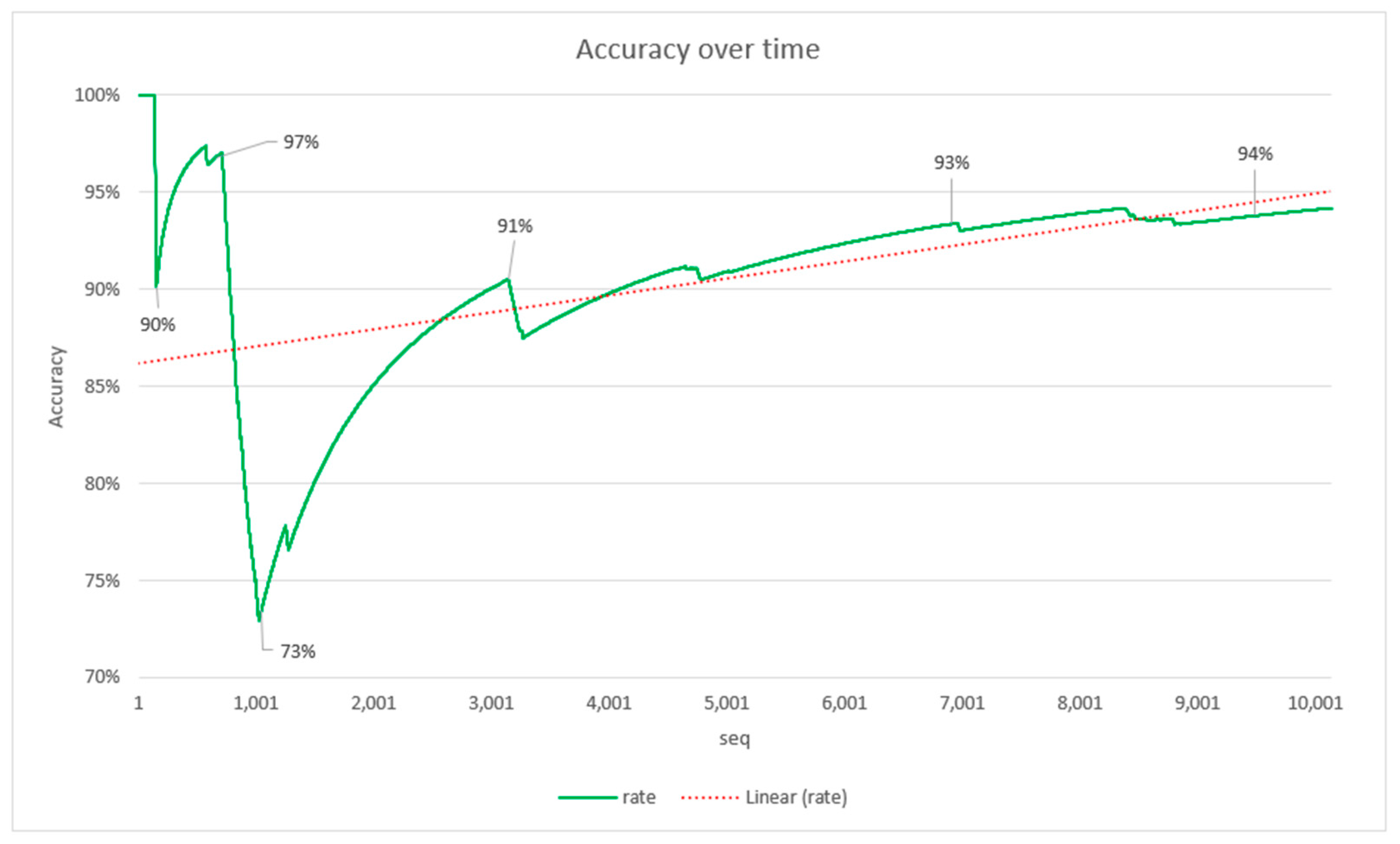
Furthermore, as FOCUSeR uses an approach of keeping your model up to date over time, as the number of samples increases, the parameters of the IQR metric are updated. As a result of this approach, when analyzing the growth of the Accuracy rate over time, it is possible to verify that there is a trend of growth in this rate (Figure 10), indicating an improvement in the results over time.

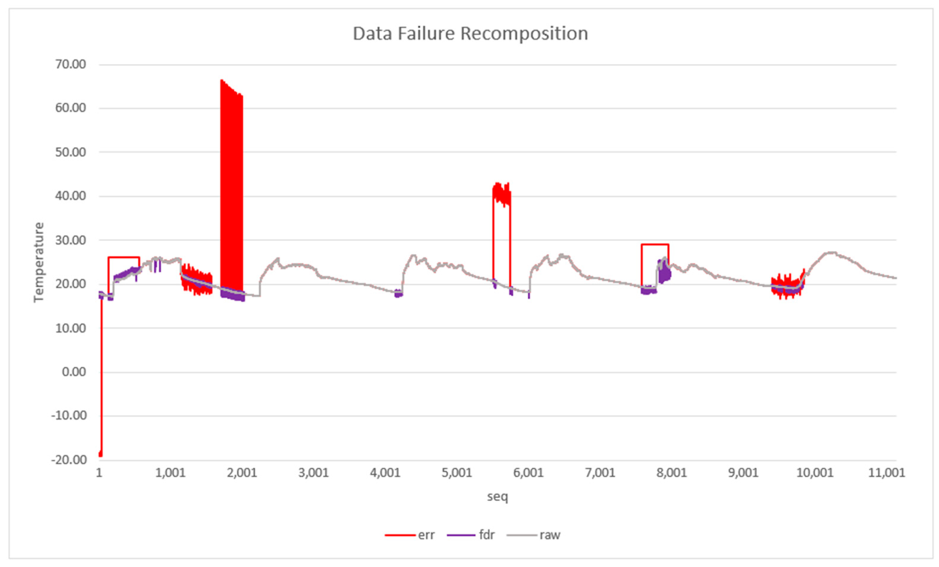
6.3. Failure Data Recomposition Evaluation

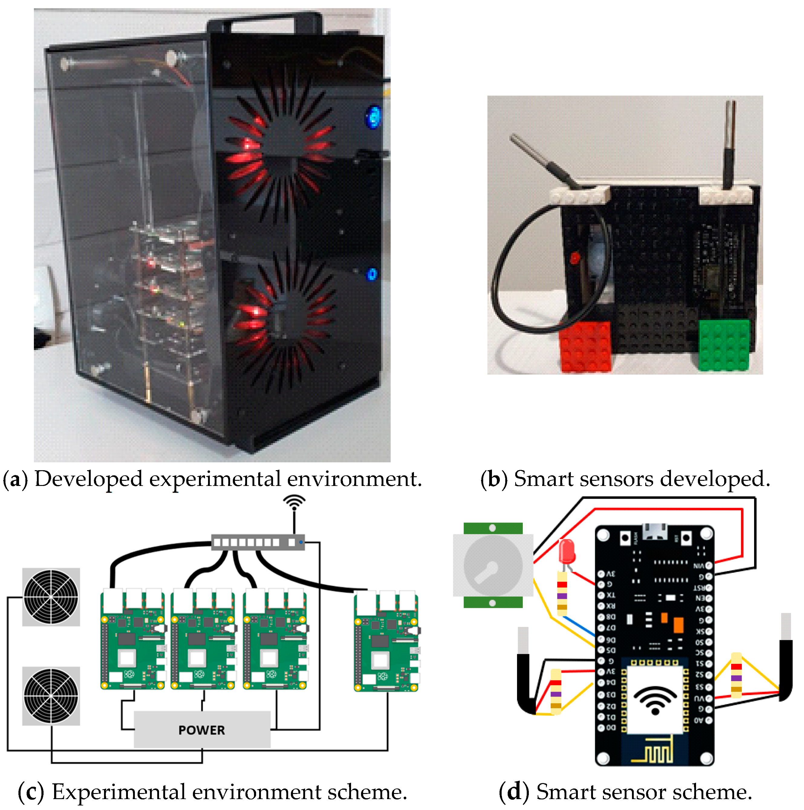
When using the active ranking approach, the algorithm looks for nearby sensors with valid (normal) values if the value read from the current sensor is considered abnormal. The scenario of this test used the processing of data in multiple nodes (raspberry’s). Each node listening to a specific sensor. In this way, data were selected if they met the requirements of geographic location, message freshness and age, that is, the QoC parameters.

Figure 11 presents a failures data recovery scenario. This graph was generated using the data files of sensor 1 of the Intel dataset available in the work of [59]. Three data sets were used to construct the graph: data without errors (gray), that is, original data from the Intel dataset, data with injected errors (red) and data generated by FOCUSeR (violet). As shown in the graph, most of the samples identified as anomalies or failures by FOCUSeR can be retrieved from nearby sensors, more precisely 87.31%.

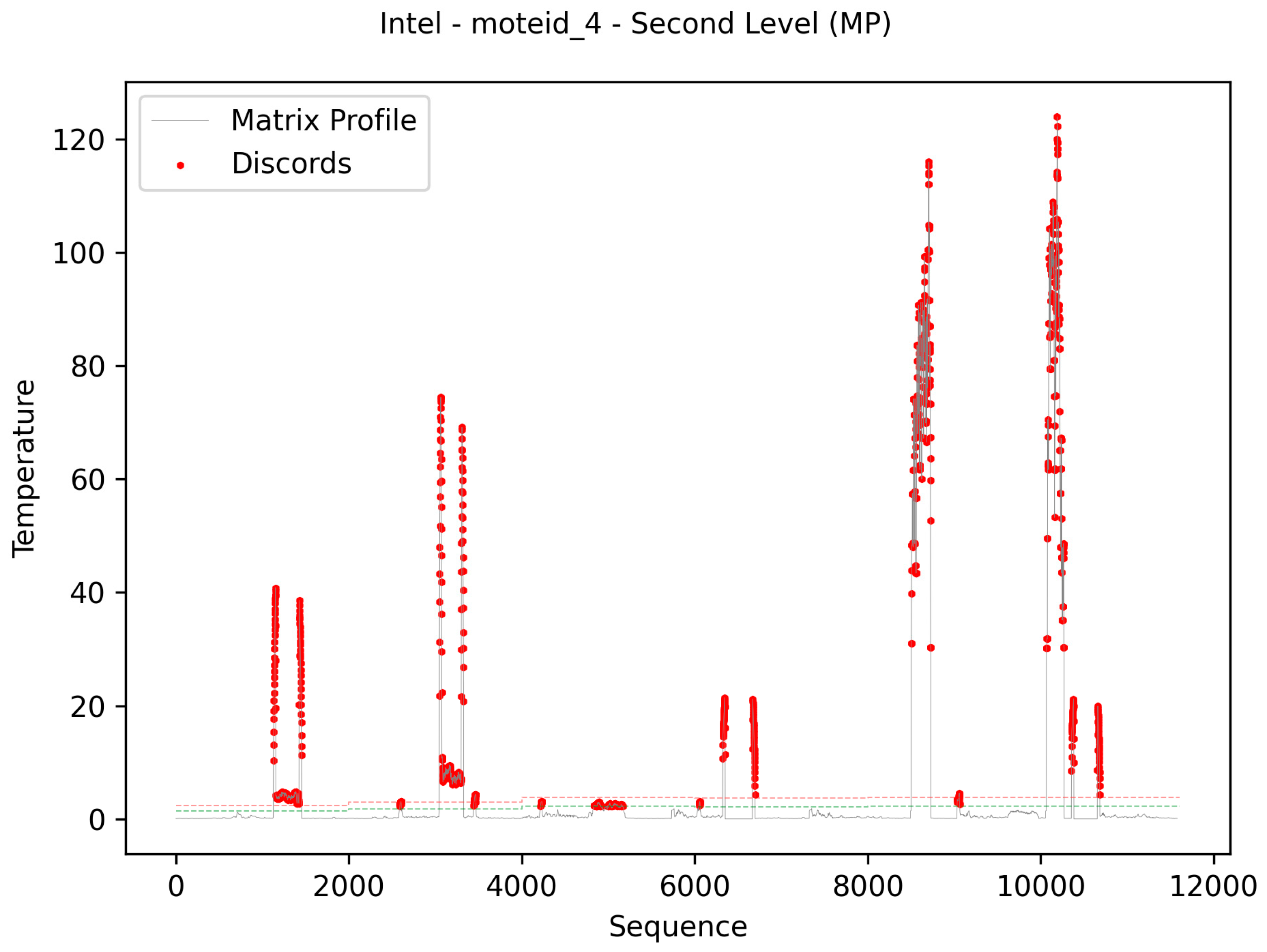
6.4. Online and Up-to-Date Approach Results

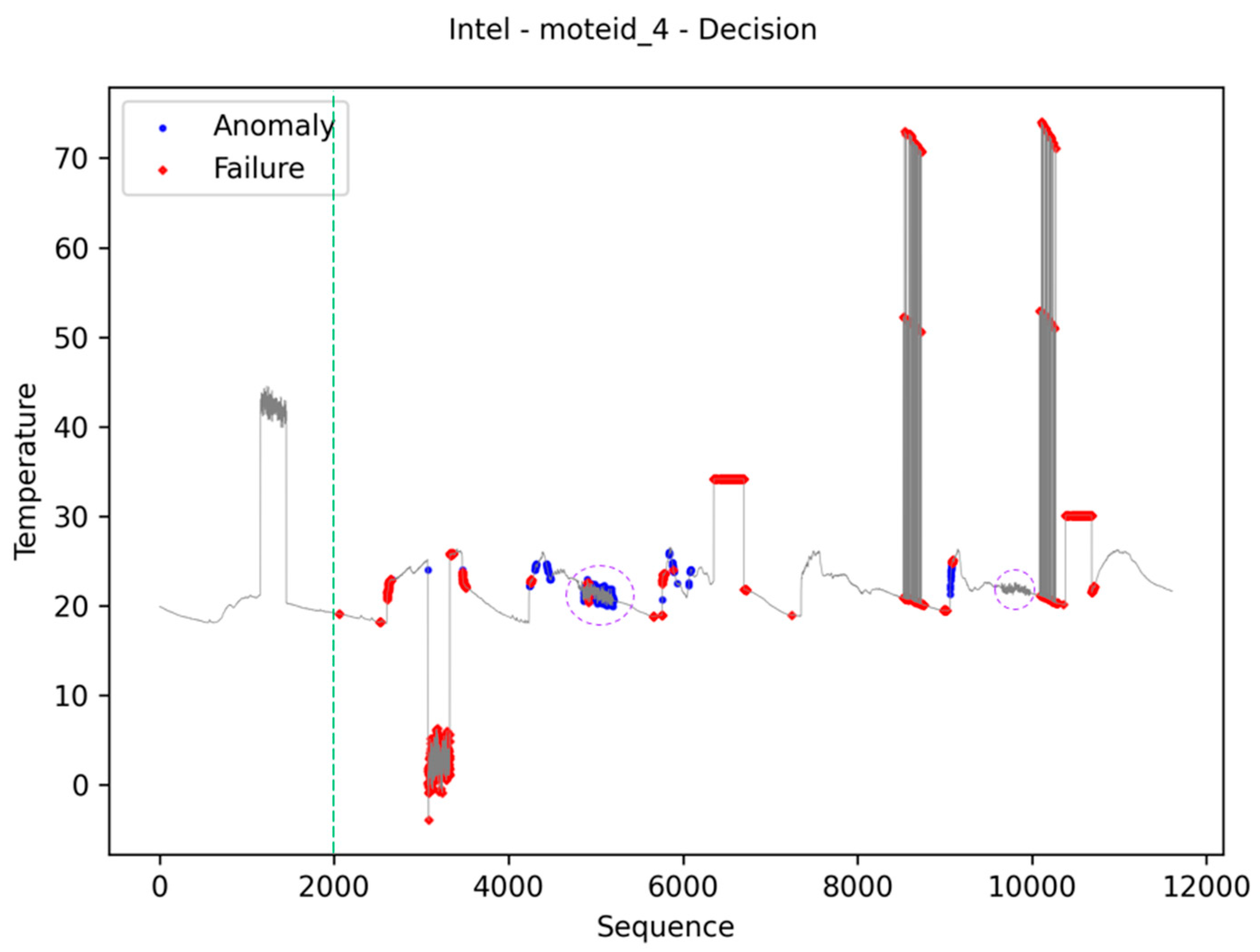
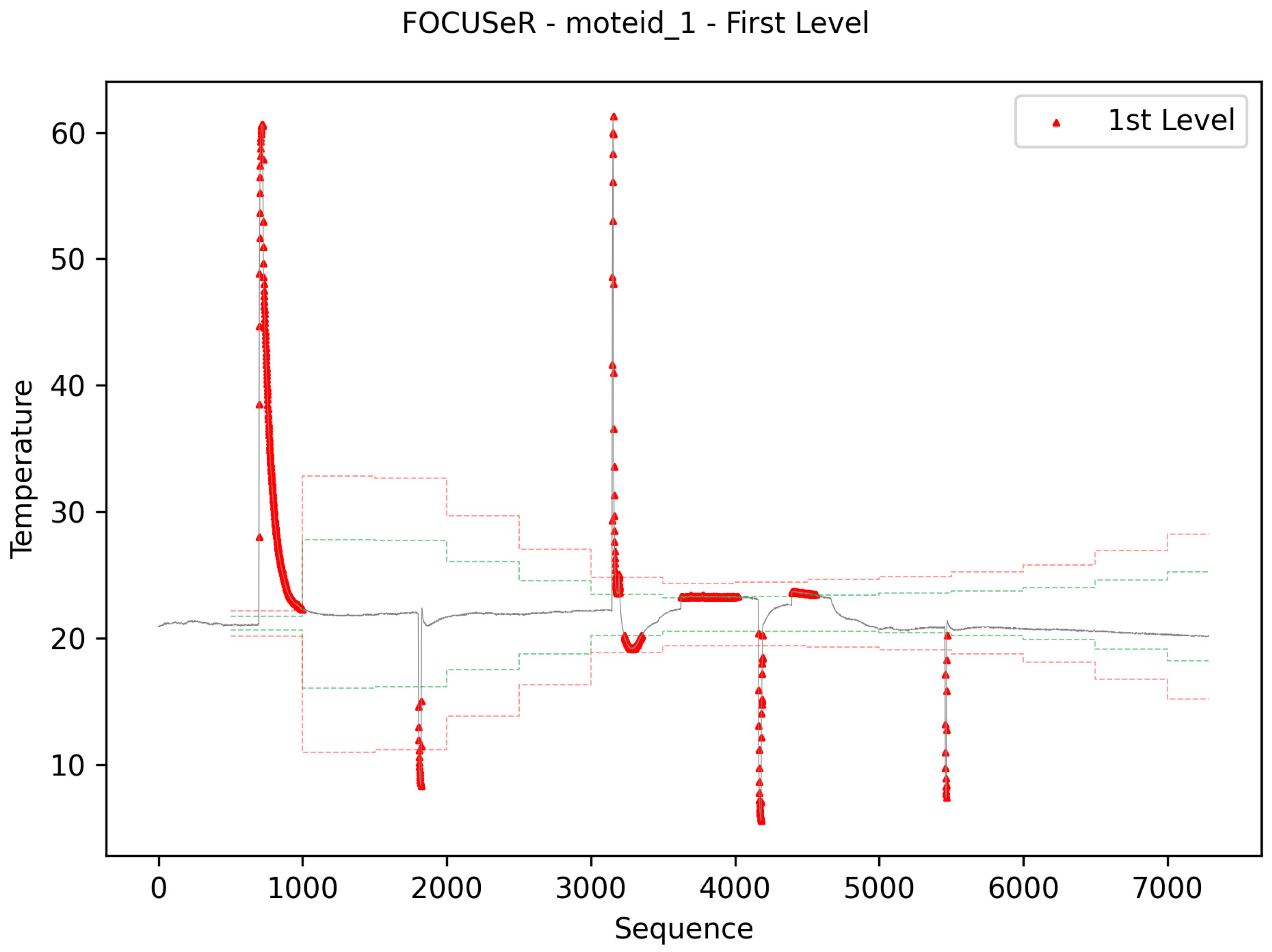
From Figure 12, Figure 13 and Figure 14, the presented images demonstrate the proposal’s online training approach, as well as the ability to keep indexes up to date. The green dashed line in Figure 12 separates the data used in the algorithm’s burn-in step from those used in normal processing. For this reason, data before this row is not labeled as anomaly and failure. The images also present the results of classifying the data into anomaly, normal, and failure. In the images, the initial data were used in the burn-in stage to generate the metrics from the IQR statistic. The green and red lines (Figure 13) represent the thresholds used to identify the data categories.

Figure 13 presents the result of the evaluation referring to the second level of the algorithm. This evaluation was performed using the matrix profile method. In the same way, the colored lines represent the limits used in the evaluation of the data. As you can see in the images, the lines have breaks at fixed-length intervals related to the burn-in parameter value. These breaks represent the updating of the IQR metric indicators. The t-digest structure was used to make it possible to update these indicators.

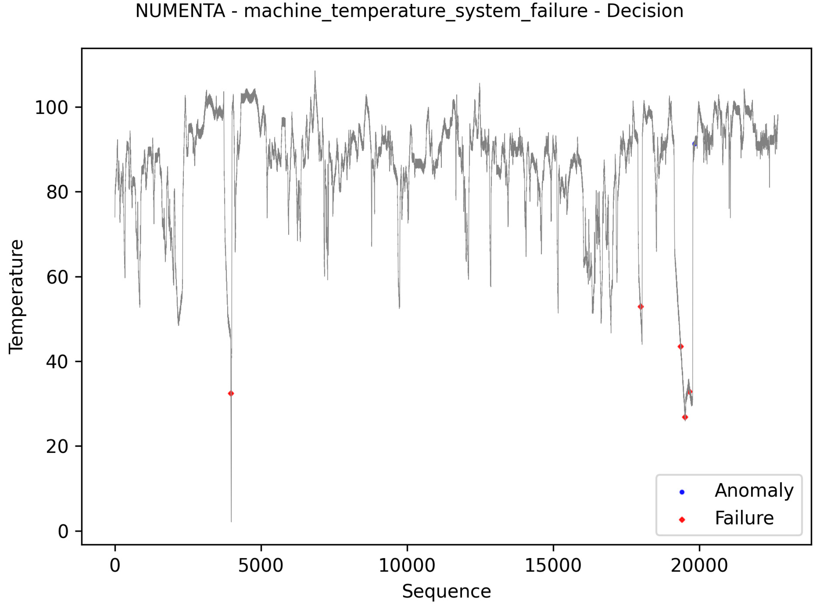
Figure 14 presents the results referring to the NUMENTA dataset. Despite the absence of labels, and for this reason it was not included in the Accuracy assessment, some works [69,70] mention the presence of three anomalies in this dataset. Comparing the results of the generated graph with that of the work of [56] it is possible to see that the first and last anomalies were identified at the same points and the second at a slightly different location. As the work states, the second anomaly is difficult to identify exactly.

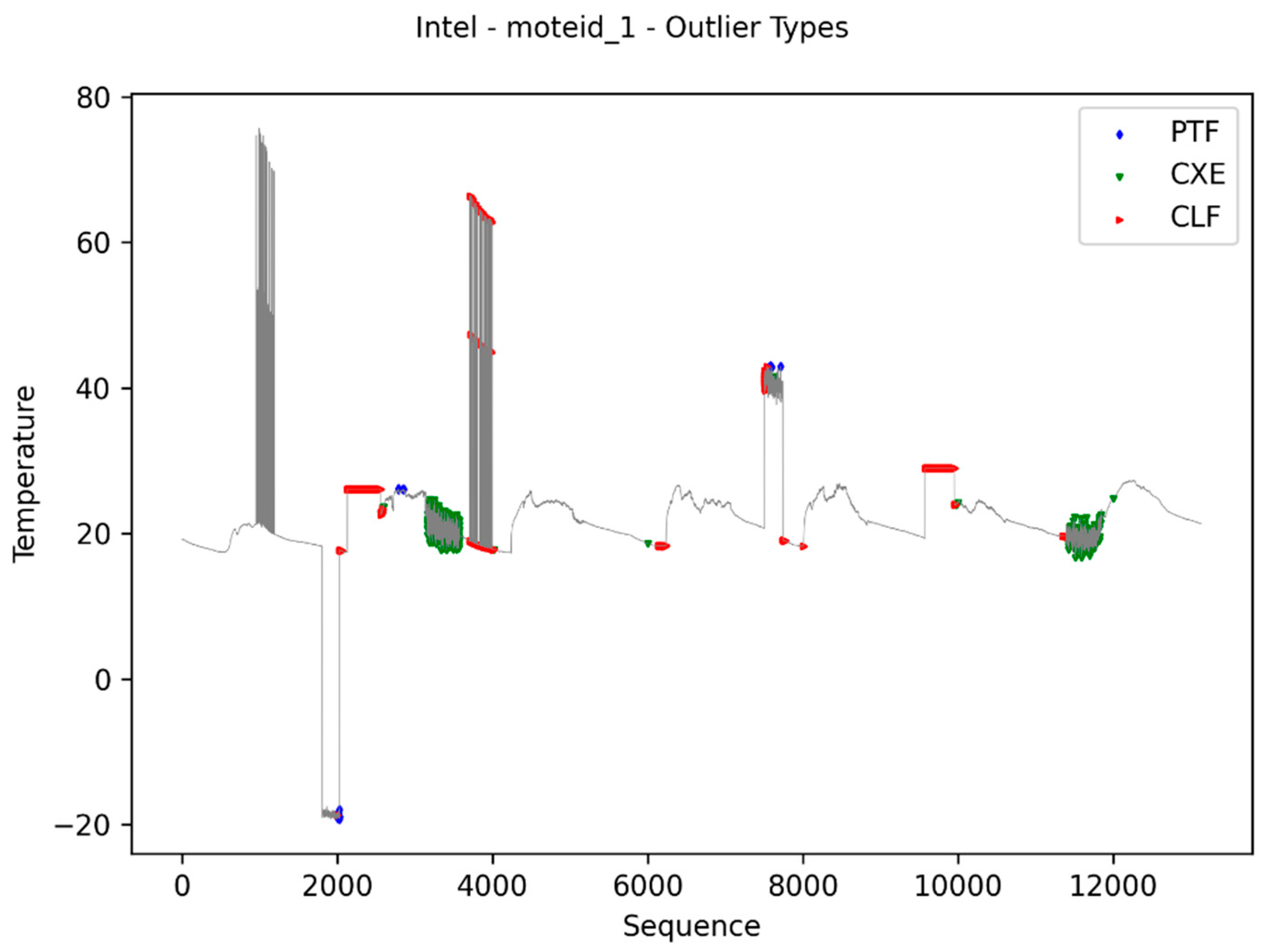
In addition to classifying the data into normal, anomaly and failure, this proposal delivers a classification of the outlier type, as shown in Figure 5.

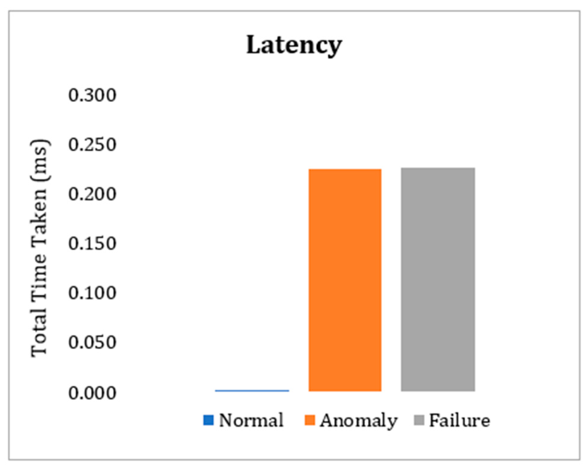
6.5. Latency Evaluation

To evaluate latency, we consider latency as the time difference between the time of entry and exit of the message in the system. In this experiment the messages were processed in the raspberry nodes configured in the developed testbed. As shown in Figure 15, the average latency added by the proposal is approximately 0.0016 milliseconds per transaction. When faults or anomalies in the readings are identified, the proposed algorithm searches for normal data in neighboring sensors. In these cases, the average latency added is approximately 0.225 milliseconds per transaction.

In the case of the average latency for querying the ranking list, the times are similar to the values of queries to data from nearby sensors since both queries are performed on the distributed hash lists.

The performance in relation to latency is not compared with other works due to the diversity of approaches in relation to the metrics used. Most of the works use the query times of the ranking list as a metric and in these cases, most of the time is spent with the sensor selection operations according to the query criteria. In addition, aspects such as network transmission speed and hardware used in the tests drastically impact the results.

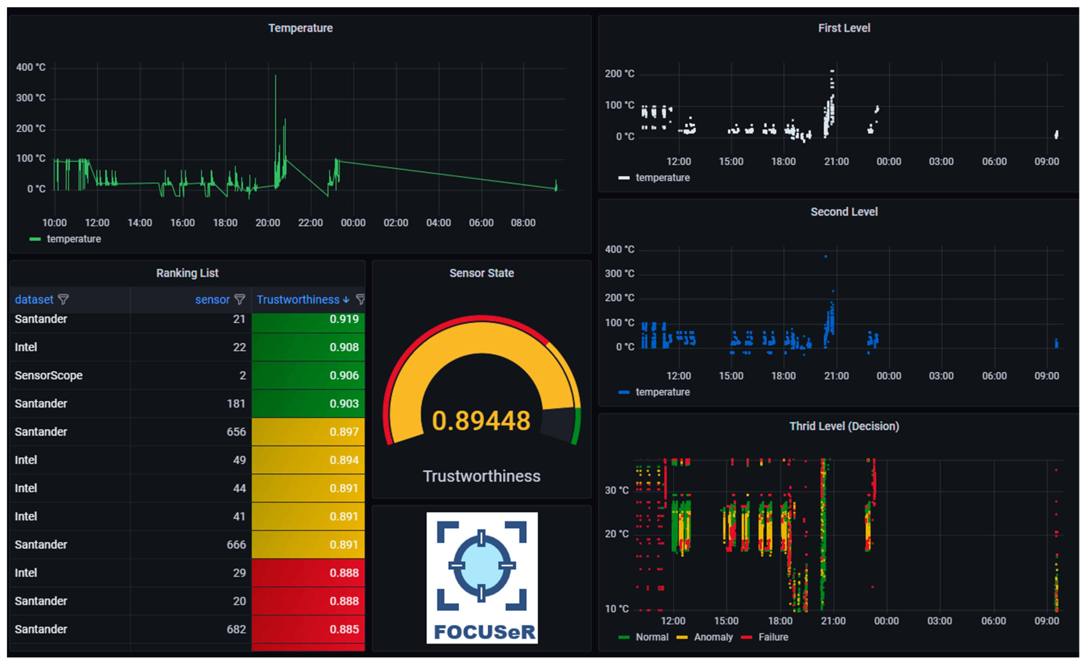
6.6. Cloud Monitoring

Finally, Figure 16 exemplifies a way of monitoring environments using the results produced by the proposal.

The monitoring panel shown in the image includes sensor value monitoring (top left); the results of the evaluation at the different levels of the proposal (right); and the ranking list of sensors classified using the trustworthiness parameter (bottom left).

7. Discussion

The method proposed in this research work can create and managing sensor ranking lists, in a distributed way, so that the information is available for services and applications as fast as possible. In the same sense, the proposed method also keeps the parameters obtained in the online training up-to-date, to prevent them from becoming outdated due to changes in the data. To the best of our knowledge, this is the first sensor ranking method that addresses all these features.

The numerical results obtained in the tests demonstrate the feasibility of the proposed method. However, the indices obtained with the Accuracy metric are slightly lower than some of the related works. In these cases, it is important to emphasize that the related works considered do not present online solutions, that is, free of training and also do not present techniques to keep the parameters updated. These requirements are fundamental given the characteristics of the IoT environment, in which the immense heterogeneous volume of sensors makes training for each sensor or even dataset unfeasible. On the other hand, FOCUSeR obtained the best values in the other metrics used.

Analyzing the results, it is possible to verify that the highest incidence occurs due to False Positive values, that is, values considered as normal when they should be considered as anomalies or failures. It is important to remember that the datasets in which this occurs are datasets with artificially inserted faults [59]. This issue occurs on failures that are considered “malfunctions” in the job from which the datasets were obtained. In this type of artificial failure, data is generated more frequently than expected. The cause of this misclassification of data is related to the magnitude of errors injected into the dataset. As can be seen in Figure 12, the dashed purple lines identify two regions where this type of error was inserted into the dataset. The first region was correctly identified, which was not the case with the second. This is due to the amplitude of the values entered, which in the case of the second region, is very small.

Regarding latency, considering the real datasets and testbed used in the tests, the response times obtained are promising and demonstrate the robustness of the proposal. This statement is supported by the following points: the proposal is intended to run in a distributed environment; with low computational resources (Fog Computing); that provides a training-free method of evaluating data that remains updated over time; and finally, that a has low computational complexity, so as not to add latency to services and applications interested in using the results produced.

8. Conclusions and Future Works

This paper describes a method for ranking sensors that uses data evaluation as a criterion for ranking. FOCUSeR offers a real ranking solution for WSNs to be executed in the Fog Computing environment, making ranking lists available in a distributed way. FOCUSeR was evaluated in a real testbed, developed with Fog nodes and temperature sensors.

The motivation for the development of this proposal is based on the fact that, although the related works in this area present promising results, there are still some challenges to be overcome in the sensor ranking area. Given the exponential growth in the volume of connected devices, the great heterogeneity of these devices and the data generated, and considering that one of the main challenges is to efficiently deliver the detected measurements with maximum fidelity, it is reasonable to assume that methods that use supervised learning will not achieve good results when used in real environments. Thus, although the methods with this approach may present slightly superior results to those of this proposal, we can assume that our method is superior, as it is free of training and has resources to keep its data evaluation indicators updated over time.

As future works, we consider executing the proposal using data from online public sensors and with a larger set of nodes for processing; increase the criteria used in the selection of spatially and temporally correlated sensors to be used to replace the values of the sensors in failure state; and we also consider the implementation of resources for the rational use of sensors, aiming to provide an energy saving mechanism.