Plant Disease Classification: A Comparative Evaluation of Convolutional Neural Networks and Deep Learning Optimizers


Abstract

1. Introduction
2. Materials and Methods
2.1. Dataset
2.2. Software and Hardware Specifications
2.3. Deep Learning Architectures
2.4. Deep Learning Optimizers
- SGD: This is one of the simplest deep learning optimizers. A static learning rate for all the parameters requires in the duration of whole training and it has a fast convergence ability [41].
- Adagrad: This optimizer uses different learning rates for every parameter in the model. It updates the learning rate according to the frequency of the update of each parameter [42].
- RMSProp: To reduce the training time observed in Adagrad, the RMSProp optimizing functions were proposed and its learning rate decays exponentially [43].
- Adadelta: This is an extended version of Adagrad optimizer and accumulates the previous gradients over a fixed time window which ultimately ensures the continuation of learning even after many iterations. Adadelta used Hessian approximation to ensure the update direction in the negative gradient and eliminated the learning rate from update rule [44].
- Adam: The Adaptive moment estimation method (Adam) evaluates adaptive learning rates from the first and second moments of gradients for various parameters [45]. It has combined advantages of two extended versions of the SGD method that are Adagrad and RMSProp. In contrast with the RMSProp, it calculates the average of the second moment of gradient and it also utilizes the previous gradients to speed up learning [45].
- Adamax: A different version of Adam was also proposed in [45] which is based on the infinity norm and could be useful for sparse parameter updates like word embeddings.
2.5. Training Specifications
3. Results and Discussion
3.1. Step-1: Comparative Analysis of Deep Learning Architectures
3.1.1. Performance of Well-Known CNN Architectures
- The Xception model attained the highest validation accuracy, F1-score, and lowest validation loss among all the well-known CNN models. Therefore, this model can be undoubtedly considered as the best CNN architecture to classify plant disease on the PlantVillage dataset. It implies that the concept of a modified version of depth-wise separable convolution [38] in the Xception model is a useful way to obtain higher classification results. Moreover, this DL model converged to its final value at the 34th epoch which is the least number of epochs as compare to all the other DL architectures. On the other hand, it required a significant amount of time to complete one epoch (around 3400 sec). Therefore, future studies should propose another version of DL architecture that can achieve Xception-level accuracy and require smaller training time for each epoch.
- The second highest F1-score/validation accuracy was attained by ZFNet architecture. Hence, a smaller filter size and the increased number of activation maps used in ZFNet architectures (as compared to AlexNet) improved its performance.
- Then, MobileNet, DenseNet, and AlexNet architectures have also achieved a good F1-score followed by Inception-v4, ResNet-50, and Inception ResNet-v2 architectures. The MobileNet is a comparatively more preferable model due to its lower number of parameters which reduced its computation time significantly. The depthwise and pointwise convolutional layers helped to achieve a better classification result. Therefore, a CNN model could be proposed in future research based on the MobileNet architecture. Moreover, this model required a lower number of epochs to achieve its final accuracy and loss as compare to DenseNet and AlexNet models (as shown in Table 2).
- The VGG-16 and OverFeat were found unsuitable models for plant disease classification as they achieved lower validation accuracy/F1-score and higher validation loss as compared to the other well-known DL architectures. The smaller filter size of the VGG model degraded its performance. However, the larger filter size of the OverFeat model significantly reduced its training time but they were not enough to provide a noticeable classification performance. Additionally, they had a higher number of parameters (in millions) which slow down their training time effectively.
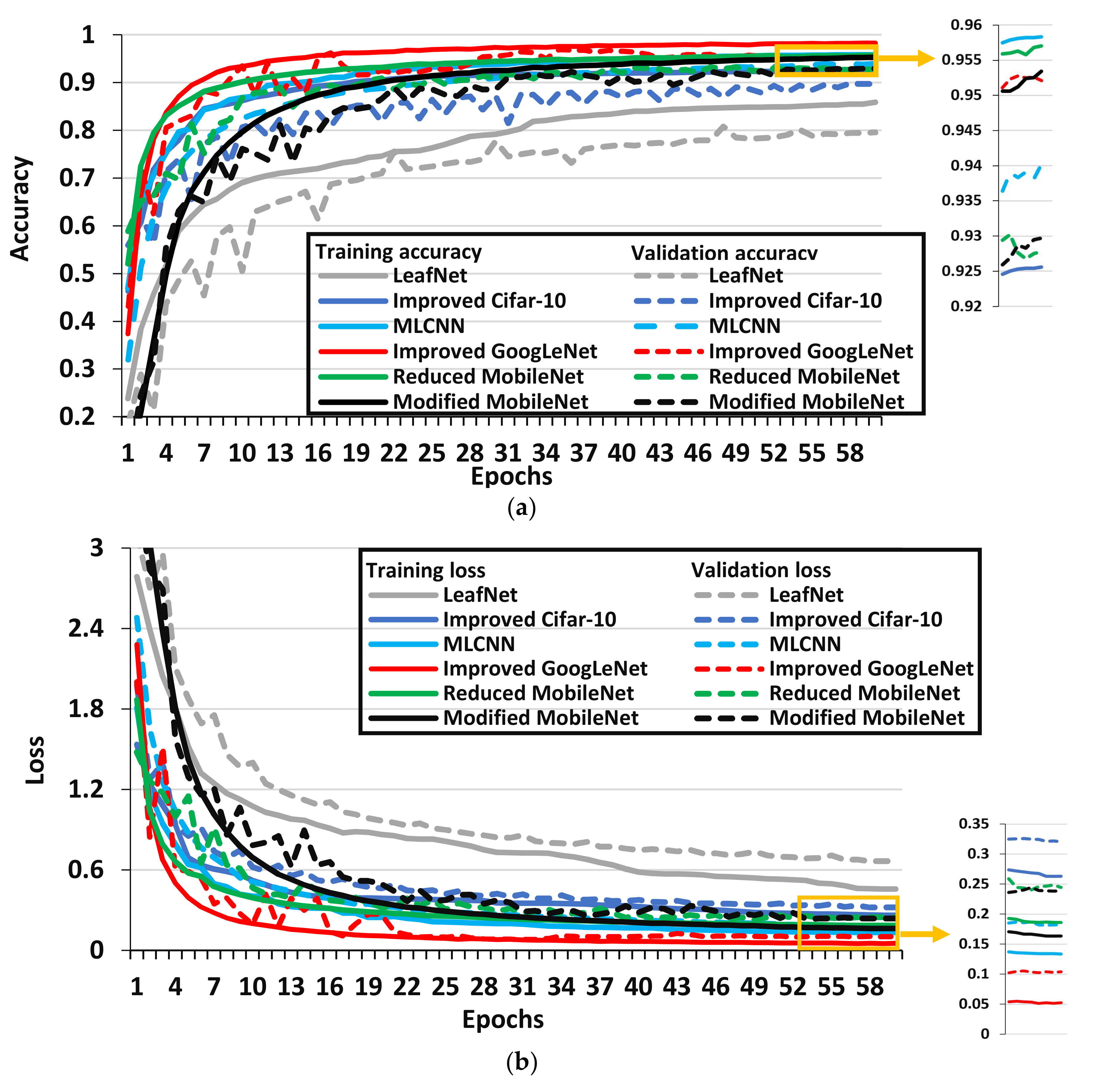
3.1.2. Performance of Modified CNN Architectures
- The improved GoogLeNet architecture achieved the best performance in terms of validation accuracy/loss and F1-score among all the modified versions of CNN architectures by utilizing the concept of the Inception module from the original GoogLeNet model. Moreover, it got the final value of accuracy and loss in 53 epochs which is the least as compared to other modified/improved versions of the DL models considered in this article, but it required more training time to complete one epoch as compared to the models like Modified and Reduced MobileNet.
- The MLCNN architecture provided a good F1-score due to the inclusion of a dropout layer after each max pooling layer and a reduction in the number of filters of the starting convolution layers in the original AlexNet architecture. However, due to a higher number of parameters, this modified DL architecture required considerably higher training time per epoch.
- The two versions of MobileNet named Modified and Reduced MobileNet models achieved an acceptable F1-score closed to each other. These modified versions of DL architecture used depthwise separable convolutional layers, which helped to attain a good classification result, and they had six times fewer parameters than the original MobileNet model which reduced their training time per epoch.
- Moreover, there were some models like Improved Cifar-10 and LeafNet models that had a lower number of parameters which increased their speed of training per epoch. The Improved Cifar-10 model achieved a noticeable F1-score, but the reduced parameters of the LeafNet model were not enough to obtain a good F1-score/validation accuracy. Therefore, it is not a suitable model to classify diseases in the selected dataset. It is also observed that these two models required a higher number of epochs as compare to other modified versions of DL architectures. Hence, future research could comprise of proposing a DL model such as Improved Cifar-10 and LeafNet for reducing the training time, but some convolutional layers should be added to attain acceptable validation/testing accuracy.
3.1.3. Performance of Cascaded/Hybrid CNN Architectures
- The cascaded AlexNet with GoogLeNet architecture outperformed all the DL models in terms of validation accuracy; moreover, except for the Xception architecture, this model achieved the highest F1-score among all the DL architectures considered in this research (as shown in Table 2). Although it required almost 57 epochs to reach its final accuracy/loss values (as shown in Figure 6), but it completed one epoch in a smaller period, which clearly shows its effectiveness in terms of training time. There were a few important modifications in the original AlexNet model, which helped to extract the features of plants containing disease including smaller convolution kernel in different layers, the inclusion of max-pooling layer, cascading the Inception module with the modified AlexNet layers, and convolutional layers after Inception to replace two fully connected layers [18].
- Moreover, a hybrid version of AlexNet with VGG architectures has also been studied, and it provided good performance in terms of validation accuracy (as shown in Figure 6) and F1-score, but it had the highest number of parameters which significantly increased its training time to complete each epoch. This model performed well due to the utilization of concepts such as normalization and selection of filter depth from AlexNet and VGG models, respectively [40].
3.2. Step-2: Improvement in Classification Results by Deep Learning Optimizers
- Considerable changes were observed in training/validation accuracy, loss, precision, recall, and F1-score by training the DL models through various deep learning optimizers.
- Adam and Adadelta were the most successful optimizers for all the three selected DL architectures.
- The Xception model trained with the Adam optimizer achieved the highest validation accuracy and F1-score of 99.81% and 0.9978, respectively, which clearly show the effectiveness of the proposed approach. Moreover, these results are better than previous studies that used the same dataset but different approaches [12,16,19,24]. Therefore, the methodology proposed in this article could be used for various other agricultural operations.
- The cascaded AlexNet with GoogLeNet and improved GoogLeNet models achieved their best classification results by using the Adadelta and Adam optimizers, respectively.
- However, a degradation in the performance has also been observed when optimizing functions were changed from SGD to Adagrad and RMSProp for Xception and cascaded models, respectively.
- It is also noticed that the Improved GoogLeNet showed its lowest validation accuracy/F1-score when it was trained by the SGD optimizer.
4. Conclusions and Future Recommendations
- Various deep learning optimizers such as Adam, and Adadelta, can also be used to enhance research on other agricultural applications, such as crop/weed discrimination, classification of weeds, plant recognition, etc.
- The classification performance of the other datasets related to plant disease could also be improved by adopting the methodology proposed in this research.
- Furthermore, although the Xception model provided the best results according to the analysis provided in this article, it required a significant amount of time to complete each epoch. Therefore, an attempt should be made to achieve an Xception level accuracy with small training time.
Author Contributions
Funding
Conflicts of Interest
References
- Liakos, K.G.; Busato, P.; Moshou, D.; Pearson, S.; Bochtis, D. Machine learning in agriculture: A review. Sensors 2018, 18, 2674. [Google Scholar] [CrossRef] [PubMed]
- Römer, C.; Bürling, K.; Hunsche, M.; Rumpf, T.; Noga, G.; Plümer, L. Robust fitting of fluorescence spectra for pre-symptomatic wheat leaf rust detection with support vector machines. Comput. Electron. Agric. 2011, 79, 180–188. [Google Scholar] [CrossRef]
- Chen, T.; Zhang, J.; Chen, Y.; Wan, S.; Zhang, L. Detection of peanut leaf spots disease using canopy hyperspectral reflectance. Comput. Electron. Agric. 2019, 156, 677–683. [Google Scholar] [CrossRef]
- Coops, N.; Stanford, M.; Old, K.; Dudzinski, M.; Culvenor, D.; Stone, C. Assessment of Dothistroma needle blight of Pinus radiata using airborne hyperspectral imagery. Phytopathology 2003, 93, 1524–1532. [Google Scholar] [CrossRef]
- Leucker, M.; Mahlein, A.-K.; Steiner, U.; Oerke, E.-C. Improvement of lesion phenotyping in Cercospora beticola–sugar beet interaction by hyperspectral imaging. Phytopathology 2015, 106, 177–184. [Google Scholar] [CrossRef] [PubMed]
- Saleem, M.H.; Potgieter, J.; Mahmood Arif, K. Plant Disease Detection and Classification by Deep Learning. Plants 2019, 8, 468. [Google Scholar] [CrossRef]
- Xie, C.; Yang, C.; He, Y. Hyperspectral imaging for classification of healthy and gray mold diseased tomato leaves with different infection severities. Comput. Electron. Agric. 2017, 135, 154–162. [Google Scholar] [CrossRef]
- Kobayashi, T.; Kanda, E.; Kitada, K.; Ishiguro, K.; Torigoe, Y. Detection of rice panicle blast with multispectral radiometer and the potential of using airborne multispectral scanners. Phytopathology 2001, 91, 316–323. [Google Scholar] [CrossRef]
- Brahimi, M.; Boukhalfa, K.; Moussaoui, A. Deep learning for tomato diseases: Classification and symptoms visualization. Appl. Artif. Intel. 2017, 31, 299–315. [Google Scholar] [CrossRef]
- Ferentinos, K.P. Deep learning models for plant disease detection and diagnosis. Comput. Electron. Agric. 2018, 145, 311–318. [Google Scholar] [CrossRef]
- Fuentes, A.; Yoon, S.; Kim, S.; Park, D. A robust deep-learning-based detector for real-time tomato plant diseases and pests recognition. Sensors 2017, 17, 2022. [Google Scholar] [CrossRef] [PubMed]
- Mohanty, S.P.; Hughes, D.P.; Salathé, M. Using deep learning for image-based plant disease detection. Front. Plant Sci. 2016, 7, 1419. [Google Scholar] [CrossRef] [PubMed]
- TÜRKOĞLU, M.; Hanbay, D. Plant disease and pest detection using deep learning-based features. Turk. J. Electr. Eng. Comput. Sci. 2019, 27, 1636–1651. [Google Scholar] [CrossRef]
- Zhang, K.; Wu, Q.; Liu, A.; Meng, X. Can Deep Learning Identify Tomato Leaf Disease? Adv. Multimed. 2018, 2018. [Google Scholar] [CrossRef]
- Oppenheim, D.; Shani, G.; Erlich, O.; Tsror, L. Using Deep Learning for Image-Based Potato Tuber Disease Detection. Phytopathology 2019, 109, 1083–1087. [Google Scholar] [CrossRef] [PubMed]
- Too, E.C.; Yujian, L.; Njuki, S.; Yingchun, L. A comparative study of fine-tuning deep learning models for plant disease identification. Comput. Electron. Agric. 2019, 161, 272–279. [Google Scholar] [CrossRef]
- Singh, U.P.; Chouhan, S.S.; Jain, S.; Jain, S. Multilayer Convolution Neural Network for the Classification of Mango Leaves Infected by Anthracnose Disease. IEEE Access 2019, 7, 43721–43729. [Google Scholar] [CrossRef]
- Liu, B.; Zhang, Y.; He, D.; Li, Y. Identification of apple leaf diseases based on deep convolutional neural networks. Symmetry 2018, 10, 11. [Google Scholar] [CrossRef]
- Geetharamani, G.; Pandian, A. Identification of plant leaf diseases using a nine-layer deep convolutional neural network. Comput. Electr. Eng. 2019, 76, 323–338. [Google Scholar]
- Zhang, X.; Qiao, Y.; Meng, F.; Fan, C.; Zhang, M. Identification of maize leaf diseases using improved deep convolutional neural networks. IEEE Access 2018, 6, 30370–30377. [Google Scholar] [CrossRef]
- Chen, J.; Liu, Q.; Gao, L. Visual Tea Leaf Disease Recognition Using a Convolutional Neural Network Model. Symmetry 2019, 11, 343. [Google Scholar] [CrossRef]
- Kamal, K.; Yin, Z.; Wu, M.; Wu, Z. Depthwise separable convolution architectures for plant disease classification. Comput. Electron. Agric. 2019, 165, 104948. [Google Scholar]
- Jiang, P.; Chen, Y.; Liu, B.; He, D.; Liang, C. Real-Time Detection of Apple Leaf Diseases Using Deep Learning Approach Based on Improved Convolutional Neural Networks. IEEE Access 2019, 7, 59069–59080. [Google Scholar] [CrossRef]
- Brahimi, M.; Arsenovic, M.; Laraba, S.; Sladojevic, S.; Boukhalfa, K.; Moussaoui, A. Deep learning for plant diseases: Detection and saliency map visualisation. In Human and Machine Learning; Springer: Berlin, Germany, 2018; pp. 93–117. [Google Scholar]
- Brahimi, M.; Mahmoudi, S.; Boukhalfa, K.; Moussaoui, A. Deep interpretable architecture for plant diseases classification. arXiv 2019, arXiv:1905.13523. [Google Scholar]
- DeChant, C.; Wiesner-Hanks, T.; Chen, S.; Stewart, E.L.; Yosinski, J.; Gore, M.A.; Nelson, R.J.; Lipson, H. Automated identification of northern leaf blight-infected maize plants from field imagery using deep learning. Phytopathology 2017, 107, 1426–1432. [Google Scholar] [CrossRef]
- Torres, J.F.; Gutiérrez-Avilés, D.; Troncoso, A.; Martínez-Álvarez, F. Random hyper-parameter search-based deep neural network for power consumption forecasting. In Proceedings of the International Work-Conference on Artificial Neural Networks (IWANN 2019), Gran Canaria, Spain, 12–14 June 2019; pp. 259–269. [Google Scholar]
- Martínez-Álvarez, F.; Asencio-Cortés, G.; Torres, J.F.; Gutiérrez-Avilés, D.; Melgar-García, L.; Pérez-Chacón, R.; Rubio-Escudero, C.; Riquelme, J.; Troncoso, A. Coronavirus optimization algorithm: A bioinspired metaheuristic based on the COVID-19 propagation model. Big Data 2020, 8, 308–322. [Google Scholar] [CrossRef]
- Hughes, D.; Salathé, M. An open access repository of images on plant health to enable the development of mobile disease diagnostics. arXiv 2015, arXiv:1511.08060. [Google Scholar]
- Krizhevsky, A.; Sutskever, I.; Hinton, G.E. Imagenet classification with deep convolutional neural networks. In Proceedings of the Advances in neural information processing systems (NIPS 2012), Lake Tahoe, NV, USA, 3–6 December 2012; pp. 1097–1105. [Google Scholar]
- Sermanet, P.; Eigen, D.; Zhang, X.; Mathieu, M.; Fergus, R.; LeCun, Y. Overfeat: Integrated recognition, localization and detection using convolutional networks. arXiv 2013, arXiv:1312.6229. [Google Scholar]
- Simonyan, K.; Zisserman, A. Very deep convolutional networks for large-scale image recognition. arXiv 2014, arXiv:1409.1556. [Google Scholar]
- Zeiler, M.D.; Fergus, R. Visualizing and understanding convolutional networks. In Proceedings of the European conference on computer vision (ECCV), Zurich, Switzerland, 6–12 September 2014; pp. 818–833. [Google Scholar]
- He, K.; Zhang, X.; Ren, S.; Sun, J. Deep residual learning for image recognition. In Proceedings of the 2016 IEEE conference on computer vision and pattern recognition (CVPR), Las Vegas, NV, USA, 26 June–1 July 2016; pp. 770–778. [Google Scholar]
- Szegedy, C.; Ioffe, S.; Vanhoucke, V.; Alemi, A.A. Inception-v4, inception-resnet and the impact of residual connections on learning. In Proceedings of the Thirty-First AAAI Conference on Artificial Intelligence (AAAI-17), San Francisco, CA, USA, 4–9 February 2017; pp. 4278–4284. [Google Scholar]
- Howard, A.G.; Zhu, M.; Chen, B.; Kalenichenko, D.; Wang, W.; Weyand, T.; Andreetto, M.; Adam, H. Mobilenets: Efficient convolutional neural networks for mobile vision applications. arXiv 2017, arXiv:1704.04861. [Google Scholar]
- Huang, G.; Liu, Z.; Van Der Maaten, L.; Weinberger, K.Q. Densely connected convolutional networks. In Proceedings of the 2017 IEEE Conference on Computer Vision and Pattern Recognition (CVPR), Hawaii Convention Center, Honolulu, HI, USA, 21–26 July 2017; pp. 4700–4708. [Google Scholar]
- Chollet, F. Xception: Deep learning with depthwise separable convolutions. In Proceedings of the 2017 IEEE Conference on Computer Vision and Pattern Recognition (CVPR), Hawaii Convention Center, Honolulu, HI, USA, 21–26 July 2017; pp. 1251–1258. [Google Scholar]
- Szegedy, C.; Liu, W.; Jia, Y.; Sermanet, P.; Reed, S.; Anguelov, D.; Erhan, D.; Vanhoucke, V.; Rabinovich, A. Going deeper with convolutions. In Proceedings of the 2015 IEEE Conference on Computer Vision and Pattern Recognition (CVPR), Boston, MA, USA, 7–12 June 2015; pp. 1–9. [Google Scholar]
- Chavan, T.R.; Nandedkar, A.V. AgroAVNET for crops and weeds classification: A step forward in automatic farming. Comput. Electron. Agric. 2018, 154, 361–372. [Google Scholar] [CrossRef]
- Ruder, S. An overview of gradient descent optimization algorithms. arXiv 2016, arXiv:1609.04747. [Google Scholar]
- Duchi, J.; Hazan, E.; Singer, Y. Adaptive subgradient methods for online learning and stochastic optimization. J. Mach. Learn. Res. 2011, 12, 2121–2159. [Google Scholar]
- Hinton, G.; Srivastava, N.; Swersky, K. Neural networks for machine learning. Available online: http://www.cs.toronto.edu/~hinton/coursera/lecture6/lec6.pdf (accessed on 5 October 2020).
- Zeiler, M.D. Adadelta: An adaptive learning rate method. arXiv 2012, arXiv:1212.5701. [Google Scholar]
- Kingma, D.P.; Ba, J. Adam: A method for stochastic optimization. arXiv 2014, arXiv:1412.6980. [Google Scholar]
- Bergstra, J.; Bengio, Y. Random search for hyper-parameter optimization. J. Mach. Learn. Res. 2012, 13, 281–305. [Google Scholar]
- Ioffe, S.; Szegedy, C. Batch normalization: Accelerating deep network training by reducing internal covariate shift. arXiv 2015, arXiv:1502.03167. [Google Scholar]


| Optimizers | Specifications |
|---|---|
| SGD | learning rate = 0.001, weight decay = 0.0005, momentum = 0.9, nesterov = False |
| Adagrad | learning rate = 0.001, epsilon = 1 × 10⁻⁷ |
| RMSProp | learning rate = 0.001, rho = 0.9, epsilon = 1 × 10⁻⁷ |
| Adadelta | learning rate = 1.0, rho=0.95, epsilon= 1 × 10⁻⁶ |
| Adam | learning rate = 0.001, beta1 = 0.9, beta2 = 0.999, epsilon = 1 × 10⁻⁸, amsgrad = False |
| Adamax | learning rate = 0.002, beta1 = 0.9, beta2 = 0.999, epsilon = 1 × 10⁻⁸ |
| Deep Learning Architectures | Parameters (in Millions) | Epochs Required to Train the Model | Training Time (in Hours) | Training Accuracy | Validation Accuracy | Training Loss | Validation Loss | Precision | Recall | F1-score |
|---|---|---|---|---|---|---|---|---|---|---|
| LeafNet | 0.324 M | 59 | 5.95 | 0.8590 | 0.7961 | 0.4563 | 0.6658 | 0.7946 | 0.7971 | 0.7958 |
| VGG-16 | 138 M | 59 | 38.13 | 0.8339 | 0.8189 | 0.5328 | 0.5651 | 0.8182 | 0.8194 | 0.8188 |
| OverFeat | 141.8 M | 58 | 6.75 | 0.8995 | 0.8603 | 0.3201 | 0.4330 | 0.8592 | 0.8628 | 0.8610 |
| Improved Cifar-10 | 2.43 M | 58 | 6.08 | 0.9256 | 0.8974 | 0.2628 | 0.3205 | 0.8944 | 0.8960 | 0.8952 |
| Inception ResNet v2 | 54.3 M | 58 | 32.83 | 0.9551 | 0.9091 | 0.1530 | 0.3047 | 0.9075 | 0.9105 | 0.9089 |
| Reduced MobileNet | 0.5 M | 55 | 11.72 | 0.9570 | 0.9278 | 0.1860 | 0.2442 | 0.9269 | 0.9267 | 0.9268 |
| Modified MobileNet | 0.5 M | 53 | 6.38 | 0.9534 | 0.9297 | 0.1632 | 0.2385 | 0.9278 | 0.9265 | 0.9271 |
| ResNet-50 | 23.6 M | 55 | 26.33 | 0.9873 | 0.9423 | 0.0468 | 0.1923 | 0.9351 | 0.9358 | 0.9354 |
| MLCNN | 78 M | 57 | 67.33 | 0.9583 | 0.9402 | 0.1335 | 0.1820 | 0.9386 | 0.9411 | 0.9398 |
| Inception v4 | 41.2 M | 59 | 52.92 | 0.9586 | 0.9489 | 0.1410 | 0.1828 | 0.9410 | 0.9466 | 0.9438 |
| Improved GoogLeNet | 6.8 M | 53 | 9.67 | 0.9829 | 0.9521 | 0.0522 | 0.1038 | 0.9528 | 0.9539 | 0.9533 |
| AlexNet | 60 M | 54 | 6.10 | 0.9689 | 0.9578 | 0.1046 | 0.1298 | 0.9563 | 0.9570 | 0.9566 |
| DenseNet-121 | 7.1 M | 56 | 28.75 | 0.9826 | 0.9580 | 0.0758 | 0.1323 | 0.9581 | 0.9569 | 0.9575 |
| MobileNet | 3.2 M | 47 | 14.70 | 0.9764 | 0.9632 | 0.0903 | 0.1090 | 0.9624 | 0.9612 | 0.9618 |
| Hybrid AlexNet with VGG (AgroAVNET) | 238 M | 54 | 49.90 | 0.9841 | 0.9649 | 0.0546 | 0.1078 | 0.9626 | 0.9674 | 0.9650 |
| ZFNet | 58.5 M | 47 | 6.47 | 0.9752 | 0.9717 | 0.0746 | 0.1139 | 0.9746 | 0.9751 | 0.9748 |
| Cascaded AlexNet and GoogLeNet | 5.6 M | 57 | 6.5 | 0.9931 | 0.9818 | 0.0229 | 0.0592 | 0.9749 | 0.9751 | 0.9750 |
| Xception | 22.8 M | 34 | 56.28 | 0.9990 | 0.9798 | 0.0140 | 0.0621 | 0.9764 | 0.9767 | 0.9765 |
| Optimizers | Training Accuracy | Validation Accuracy | Training Loss | Validation Loss | Precision | Recall | F1-score |
|---|---|---|---|---|---|---|---|
| Cascaded AlexNet with GoogLeNet | |||||||
| SGD | 0.9931 | 0.9818 | 0.0229 | 0.0592 | 0.9749 | 0.9751 | 0.9750 |
| RMSProp | 0.9894 | 0.9757 | 0.0482 | 0.1479 | 0.9746 | 0.9613 | 0.9679 |
| Adagrad | 0.9956 | 0.9824 | 0.0153 | 0.0547 | 0.9815 | 0.9782 | 0.9798 |
| Adamax | 0.9990 | 0.9859 | 0.0029 | 0.0574 | 0.9828 | 0.9795 | 0.9811 |
| Adam | 0.9989 | 0.9857 | 0.0039 | 0.0750 | 0.9836 | 0.9836 | 0.9836 |
| Adadelta | 0.9993 | 0.9873 | 0.0024 | 0.0696 | 0.9846 | 0.9856 | 0.9851 |
| Improved GoogLeNet | |||||||
| SGD | 0.9829 | 0.9521 | 0.0522 | 0.1038 | 0.9528 | 0.9539 | 0.9533 |
| RMSProp | 0.9723 | 0.9685 | 0.1780 | 0.2272 | 0.9692 | 0.9666 | 0.9679 |
| Adagrad | 0.9889 | 0.9718 | 0.0350 | 0.0930 | 0.9651 | 0.9618 | 0.9634 |
| Adamax | 0.9998 | 0.9847 | 8.782 × 10⁻⁴ | 0.0875 | 0.9792 | 0.9826 | 0.9809 |
| Adam | 0.9992 | 0.9904 | 0.0026 | 0.0434 | 0.9859 | 0.9872 | 0.9864 |
| Adadelta | 0.9991 | 0.9905 | 0.0022 | 0.0567 | 0.9828 | 0.9879 | 0.9861 |
| Xception | |||||||
| SGD | 0.9990 | 0.9798 | 0.0140 | 0.0621 | 0.9764 | 0.9767 | 0.9765 |
| RMSProp | 0.9998 | 0.9924 | 6.922 × 10⁻⁴ | 0.0433 | 0.9877 | 0.9920 | 0.9900 |
| Adagrad | 0.9987 | 0.9621 | 0.0164 | 0.1460 | 0.9682 | 0.9505 | 0.9593 |
| Adamax | 1.0000 | 0.9889 | 0.0012 | 0.0415 | 0.9902 | 0.9874 | 0.9888 |
| Adam | 1.0000 | 0.9981 | 6.890 × 10⁻⁴ | 0.0178 | 0.9981 | 0.9975 | 0.9978 |
| Adadelta | 1.0000 | 0.9906 | 8.407 × 10⁻⁴ | 0.0364 | 0.9926 | 0.9887 | 0.9906 |
© 2020 by the authors. Licensee MDPI, Basel, Switzerland. This article is an open access article distributed under the terms and conditions of the Creative Commons Attribution (CC BY) license (http://creativecommons.org/licenses/by/4.0/).
Share and Cite
Saleem, M.H.; Potgieter, J.; Arif, K.M. Plant Disease Classification: A Comparative Evaluation of Convolutional Neural Networks and Deep Learning Optimizers. Plants 2020, 9, 1319. https://doi.org/10.3390/plants9101319
Saleem MH, Potgieter J, Arif KM. Plant Disease Classification: A Comparative Evaluation of Convolutional Neural Networks and Deep Learning Optimizers. Plants. 2020; 9(10):1319. https://doi.org/10.3390/plants9101319
Chicago/Turabian StyleSaleem, Muhammad Hammad, Johan Potgieter, and Khalid Mahmood Arif. 2020. "Plant Disease Classification: A Comparative Evaluation of Convolutional Neural Networks and Deep Learning Optimizers" Plants 9, no. 10: 1319. https://doi.org/10.3390/plants9101319
APA StyleSaleem, M. H., Potgieter, J., & Arif, K. M. (2020). Plant Disease Classification: A Comparative Evaluation of Convolutional Neural Networks and Deep Learning Optimizers. Plants, 9(10), 1319. https://doi.org/10.3390/plants9101319