Early Eocene Palynofloral Diversity and Nothofagus Niche Modeling Across Western Gondwana

Abstract

During warm intervals such as the Early Eocene, megathermal vegetation belts expanded toward higher latitudes, displacing mesothermal and microthermal biota. Here, we examine the diversity and paleoclimate of the Early Eocene Ligorio Márquez Formation (LMF) in the context of other Paleogene Patagonian palynofloras, and we model the potential distribution of Nothofagus using Early Eocene climate simulations. From 35 processed samples, 20 yielded palynomorphs and 85 morphospecies were distinguished. We hypothesize that species richness in the LMF is comparable to other Eocene microfloras, and that climate models will confirm mesothermal conditions for this formation while identifying western Gondwana as the primary region of climatic suitability for Nothofagus. Our results indicate that the LMF hosted a diverse flora under mesothermal, humid-temperate conditions (Köppen–Geiger climate Cfa, within the broader Cf no-dry-season regime). Ecological niche modeling further indicates that western Gondwana (South America, the Antarctic Peninsula, New Zealand, and Australia) provided broadly suitable climatic conditions for Nothofagus. In Experiment 1 (modern-to-Eocene transfer), Maxnet models showed high discriminatory power (AUC_test = 0.86–0.88) with low omission at P10 (OR_P10 = 0.099–0.128). In Experiment 2 (Eocene-to-Eocene calibration), performance was consistently high across GCMs (AUC_test = 0.87–0.98; OR_P10 = 0.091–0.182). However, conditions across Antarctica were likely challenging, limiting its effectiveness as a dispersal corridor during the Eocene. Finally, our results suggest that the ancient South Pacific High influenced the northern distributional limit of Nothofagus in South America.

1. Introduction

Throughout the Cenozoic, the climate transitioned from a “hothouse” to an “icehouse”, a period marked by ice sheets at both poles, driven by geological and orbital processes [1,2]. The marine δ¹⁸O record exhibits several steps and peaks that mirror global climatic changes, encompassing ice-sheet expansion and retreat and a significant decrease in δ¹³C within continental sediments [2]. The Hothouse occurred between the Paleocene-Eocene Thermal Maximum at 56 Ma and the end of the Early Eocene Climate Optimum (EECO) at 47 Ma, when temperatures were more than 10 °C warmer than they are today and displayed greater amplitude variability [1]. During this period, the pCO₂ reached values up to 720 ppm with a peak of 1600 ppm at ~51 Ma during the EECO [3].

It has been postulated that during warmer periods, such as the Early Eocene, vegetational belts with biota adapted to megathermal climates (i.e., Mean Annual Temperature (MAT) > 22 °C, ref. [4] would expand their distribution toward higher latitudes. This expansion would result in the displacement of mesothermal (MAT 14–22 °C)—microthermal (MAT < 14 °C) biota to even higher latitudes [5,6,7]. Under this scenario, species richness, which refers to the diversity of species within a particular area, would be greater during warmer periods in mid-latitudes [5,7,8,9].

Fossil records from the South American tropics show increased plant diversity and origination rates between the Upper Paleocene and Lower Eocene flora [10,11]. This trend displays a diversity peak during the Paleogene, with values surpassing those of Holocene records in the same area [10,12]. Simultaneously, in southern South America, fossil evidence reveals high levels of diversity in paleontological records during the Eocene. The number of mammalian genera increased significantly from preceding levels at the onset of the Eocene Climatic Optimum [13]. Plant–insect associations in the Patagonian Eocene ecosystem demonstrate heightened richness, comparable to modern associations in tropical and subtropical forests [14]. Furthermore, fossil flora from Argentina’s Patagonia, specifically at Laguna del Hunco and Río Pichileufú, provide compelling macrofossil evidence for the ancient history of high plant diversity at mid-high latitudes during the Eocene of South America [14,15,16].

Numerous models have been proposed to elucidate the relationship between vegetation response and climatic changes in southern South America throughout the Paleogene–early Neogene [17,18,19,20,21,22,23]. Paleophytogeographical models indicate a temporal and spatial succession of distinct paleofloristic assemblages, ranging from Gondwanan to Mixed and Subtropical Neogene floras [18,21,24].

The succession of these floras is closely tied to at least three climatic scenarios. First, mesothermal conditions prevailed during the Paleocene–early Eocene climatic optimum. Second, the Eocene–Oligocene transition saw temperate and drier conditions due to Antarctic glaciation. Third, a cooling trend marked the end of the Neogene epoch, punctuated by a warm climatic optimum in the Middle Miocene, characterized by a temperature increase of 6–9 °C compared to the Oligocene epoch [18,21].

The paleofloristic sequence described above has been replicated in the palynological record during the Cenozoic in Patagonia [21]. From the Paleocene to Early Eocene, a Gondwana Paleoflora inhabited southern South America. This flora included lineages such as Podocarpaceae, Araucariaceae, Cunoniaceae, and Proteaceae, along with tropical-subtropical taxa like Arecaceae and Myricaceae.

A significant shift occurred in the Middle Eocene, marked by a rapid transition from the Gondwana Paleoflora to a Mixed Paleoflora, which persisted until the Oligocene. This transition featured the prevalence of the Nothofagaceae family in the palynological record and the gradual replacement of mega-mesothermal communities by microthermal rainforests [25].

By the Late Oligocene to Early Miocene, warm climates facilitated the southward dispersal of some neotropical elements. These included palms, Cupania, Alchornea, Rubiaceae, and Combretaceae, introducing megathermal elements to the existing local floras. The eventual disappearance of mega-mesothermal elements in Patagonia characterized Miocene palynofloras. This period also saw increased diversity and abundance of xerophytic taxa, such as Asteraceae, Chenopodiaceae, and Convolvulaceae [21,25].

The Ligorio Márquez Formation (LMF), named after the coal mine located in Chilean Patagonia (46°45′ S; 71°50′ W), records the earliest deposits of the lower Paleogene identified in the Chilean Patagonia region [26,27] (see Section 4 for age discussion).

Ligorio Marquez flora thrived in warm, humid, frost-free, mesothermal climates during the Early Eocene. At that time, the Mean Annual Temperature was approximately 17° to 20 °C, with Annual Precipitation exceeding 1500 mm. The presence of Nothofagus in the LMF marks the northern distribution limit of the taxon in South America during the Early Eocene. This suggests that floras with the iconic Gondwana taxa Nothofagus occupied the southern landmasses of western Gondwana during the Hothouse time of the Early Eocene, including areas such as southern South America, Antarctica, and Australia. In contrast, species from floras without Nothofagus (such as the one from Laguna del Hunco) not only expanded their distribution toward higher latitudes but also reached their southernmost limits during this period [23,28].

The development of standardized paleoclimate modeling frameworks for key moments of Earth’s history, such as the Early Eocene, which generate gridded climate fields under harmonized boundary conditions and multiple CO₂ forcings [29]. Together with emerging AI-enabled analytical workflows that facilitate synthesis across heterogeneous biodiversity data [30], these simulations provide a valuable, independent line of evidence to evaluate paleoclimate reconstructions for southern South America and to conduct spatially explicit tests of paleobiogeographic hypotheses that help us understand the effects of latitudinal shifts in thermal belts and changes in habitat suitability for key lineages, such as Gondwana taxa like Nothofagus.

Building on this framework, the Ligorio Márquez Formation (LMF) provides a well-constrained case study to evaluate whether independent paleoclimate simulations and biotic data converge on a consistent ecological and biogeographic interpretation. Here we ask whether the Early Eocene climate, under both 3× and 6× pre-industrial pCO₂ scenarios, provides a coherent mechanistic framework to explain (i) the ecological signal recorded by the LMF palynoflora and (ii) the spatial distribution of climatically suitable habitats for Nothofagus across Gondwana.

To address this question, we (1) compare palynological diversity of the LMF with other Eocene Patagonian assemblages using rarefaction-based inference; (2) evaluate published LMF paleoclimate estimates against DeepMIP–Eocene simulations [29] under 3× pre-industrial CO₂ (~800 ppm; seven models) and 6× pre-industrial (~1600 ppm; three models, approximating EECO conditions); and (3) develop ecological niche models for Nothofagus and project habitat suitability onto Early Eocene climates across Gondwana.

We hypothesized that the Early Eocene climate generated mesothermal, humid conditions at LMF and a geographically structured belt of suitable habitats for Nothofagus across western Gondwana. This hypothesis yields three linked predictions: (1) LMF species richness is comparable to other highly diverse Eocene Patagonian palynofloras (i.e., no statistical difference in rarefied richness among “Hothouse” assemblages); (2) DeepMIP simulations under both 3× and 6× pre-industrial pCO₂ reproduce mesothermal conditions at LMF (mean annual temperature between 14 °C and 22 °C, with annual precipitation exceeding 1000 mm); and (3) projected climatic suitability for Nothofagus is concentrated in western Gondwana, specifically southern South America, Antarctica, Australia, and New Zealand, thereby constraining the most plausible regions for dispersal and persistence during the Early Eocene.

2. Results

2.1. Rarefied Richness Across Eocene Hothouse Assemblages

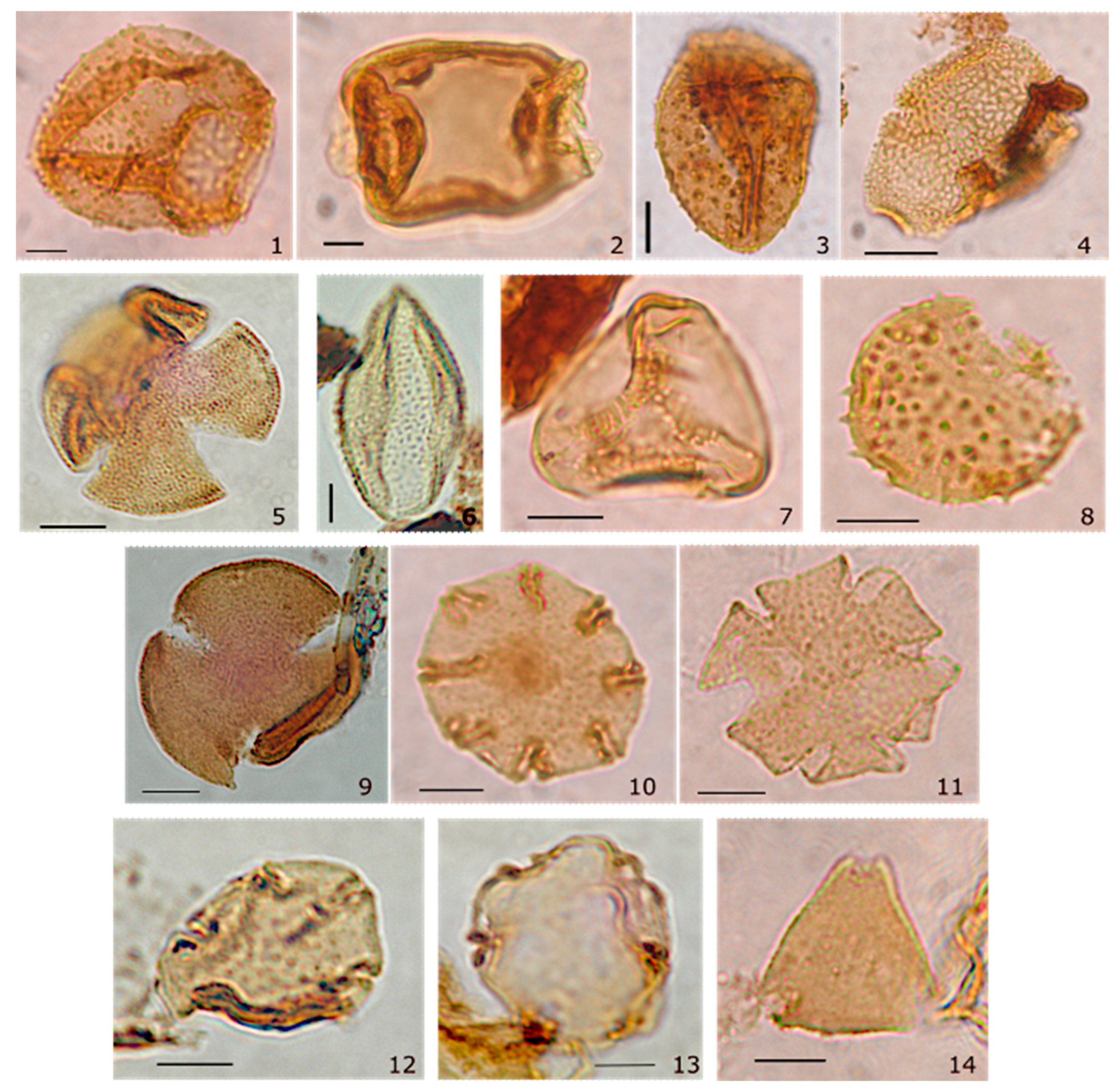
From the 35 palynological samples processed from the LMF, 20 yielded palynomorphs. A total of 85 morphospecies were distinguished in LMF, grouped as follows: 30 morphospecies of spores, 13 species of gymnosperm pollen grains, and 42 angiosperms. Other indeterminate spores and grain corresponding to algae spores, fungi, gymnosperm, and angiosperm were recovered from LMF (Figure 1, Support Information Figure S1). The total of morphospecies for LMF, considering the presence reported previously [31,32], reaches 119 taxa (Tables S1 and S2 in Support Information).

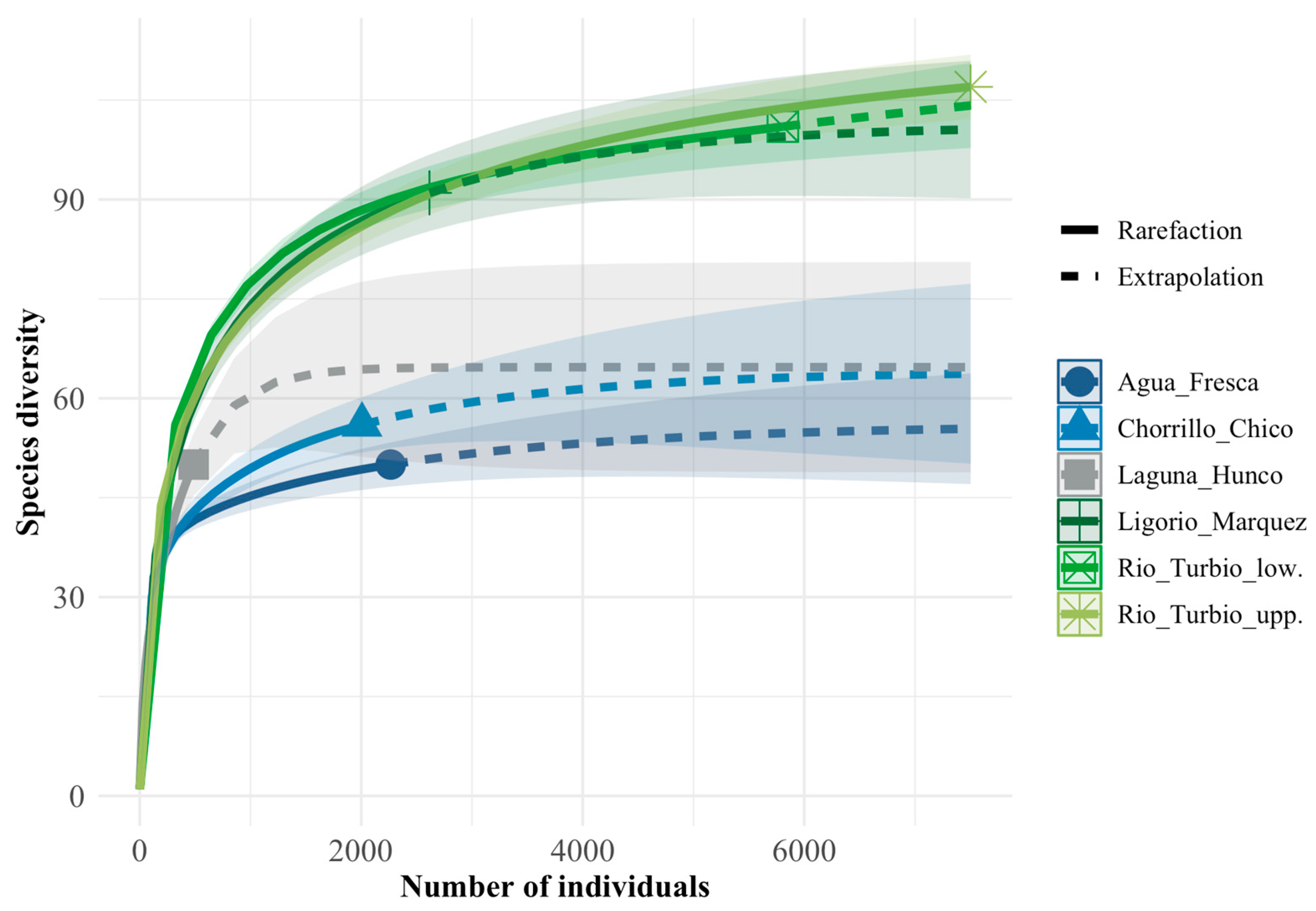
The rarefaction analysis (Figure 2) shows that LMF has no difference in species richness compared to the Rio Turbio Formation. In contrast, LMF shows higher richness than the Paleocene–early Eocene assemblages from Chorrillo Chico and Agua Fresca. Laguna del Hunco appears to have lower richness, but it could not be included in the standardized pairwise tests (see below).

Pairwise comparisons of rarefied species richness (q = 0) standardized to m₀ = 2007 individuals are summarized in

Table 1. Pairwise comparisons of rarefied species richness (q = 0) among microfloral assemblages at a common sample size (m₀ = 2007 individuals). Δ = SA(m₀) − SB(m₀), where SX(m₀) is the rarefied richness of assemblage X at m₀. Uncertainty corresponds to the bootstrap 95% confidence interval (CI95). Two-sided p-values are based on the bootstrap distribution of Δ(p), and p_Bonf indicates p-values adjusted for multiple pairwise tests using the Bonferroni procedure. Microflora compared: Ligorio Marquez Formation (LMF); Chorrillo Chico (CC); Agua Fresca (AF); Rio Turbio Formation lower and upper (RTlow and RTupp).

Comparison	m0	Δ	CI95	p	p_Bonf
LMF. vs. CC	2007	28.6	[22.8, 34.3]	<0.005	<0.005
LMF vs. AF	2007	33.6	[28.5, 38.0]	<0.005	<0.005
RTinf vs. CC	2007	33.7	[29.6, 37.8]	<0.005	<0.005
RTinf vs. AF	2007	38.7	[35.3, 42.4]	<0.005	<0.005
CC vs. RTsup	2007	−32.4	[−36.5, −28.0]	<0.005	<0.005
AF vs. RTsup	2007	−37.4	[−41.3, −33.5]	<0.005	<0.005
CC vs. AF	2007	5.0	[0.8, 9.3]	0.01	0.1
LMF vs. RTinf	2007	−5.1	[−10.7, −0.3]	0.04	0.4
LMF vs. RTsup	2007	−3.8	[−9.6, 0.7]	0.13	1
RTinf vs. RTsup	2007	1.4	[−2.5, 5.2]	0.47	1

. Using Δ = S_A(m₀) − S_B(m₀), Ligorio Márquez (LMF) and Río Turbio lower (RT_low) show higher rarefied richness than Chorrillo Chico (CC) and Agua Fresca (AF) (Δ = 28.6–38.7; all p < 0.005 and p_Bonf < 0.005). Río Turbio upper (RT_upp) also shows higher rarefied richness than CC and AF (CC vs. RTsup: Δ = −32.4; AF vs. RTsup: Δ = −37.4; both p < 0.005 and p_Bonf < 0.005). The remaining contrasts were not significant after Bonferroni correction (Table 1). Assemblage-level sampling effort and richness (N, S_obs, and S(m0) with 95% bootstrap CIs) are reported in Table S3.

Finally, Laguna del Hunco was excluded from the standardized pairwise rarefaction comparisons because its total abundance fell below the predefined minimum-sample-size threshold; therefore, it could not be compared at m₀ = 2007 without extrapolation.

2.2. Mesothermal, Humid Conditions at LMF in 3× and 6× pCO₂ DeepMIP Simulations

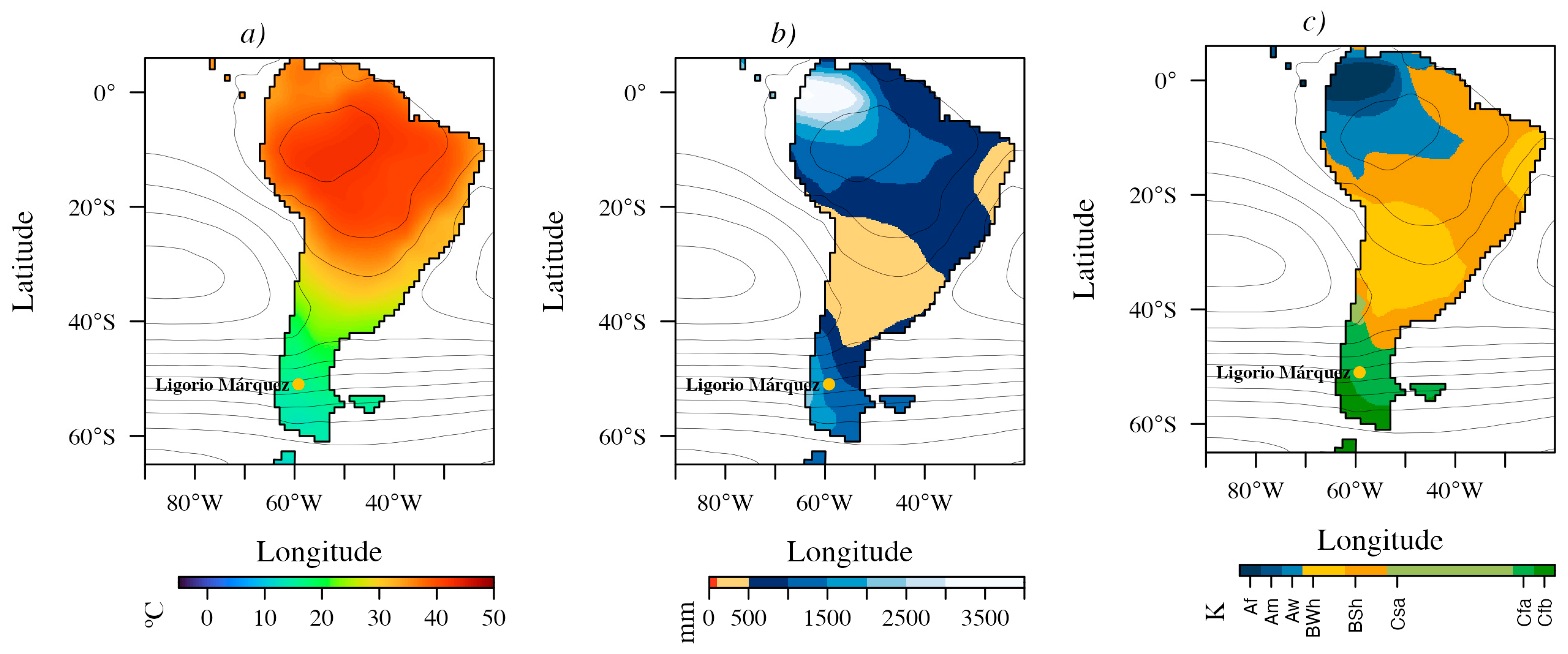
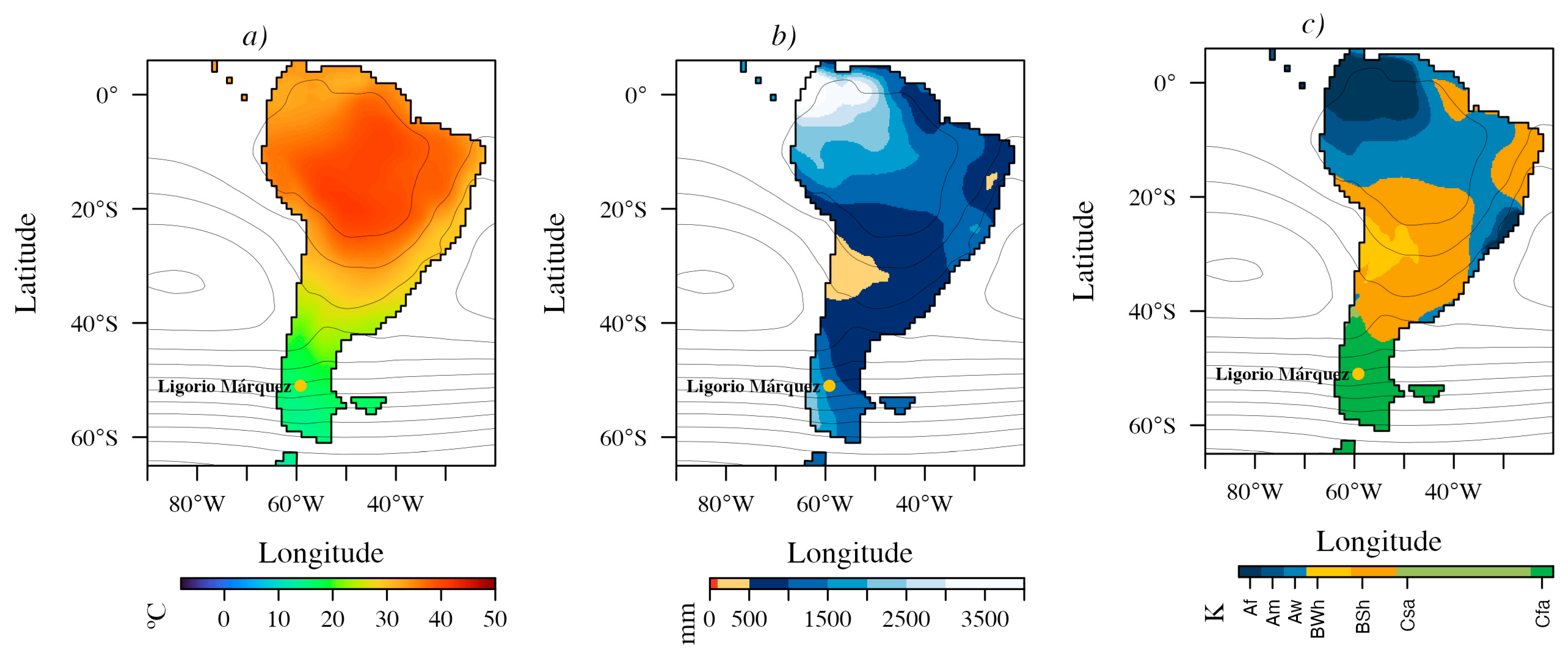
The ensemble means of seven 3 × CO₂ and three 6 × CO₂ DeepMIP simulations (Figure 3 and Figure 4) indicate predominantly megathermal conditions (mean annual temperature, MAT, 22–40 °C) across the low to mid-latitudes of South America (6° N to ~40° S), grading into mesothermal climates (14–22 °C) south of 40° S. In the 3 × CO₂ simulations, microthermal conditions (MAT < 14 °C) emerge at the southern tip of South America (~61° S) and prevail across most of Antarctica. In the 6 × CO₂ simulations, this transition shifts farther south, into the Antarctic Peninsula (~64° S).

Both ensembles also resolve an arid belt near ~30° S, consistent with the influence of the Southeast Pacific Subtropical Anticyclone. Relative to the 3 × CO₂ ensemble, the 6 × CO₂ ensemble yields generally warmer conditions over the continent and increased moisture availability around ~30° S, with annual precipitation of ~500–1000 mm (Figure 4b). In contrast, south of ~40° S annual precipitation is consistently high, ranging from ~1000 to 2500 mm under 3 × CO₂ and from ~1000 to 3000 mm under 6 × CO₂ (Figure 3b and Figure 4b).

Köppen–Geiger classifications for the Early Eocene of South America are dominated by three broad climate groups: Tropical (A), Arid (B), and Temperate (C), whose spatial extents vary between pCO₂ scenarios (Figure 3c and Figure 4c). Under 3 × CO₂ conditions (Figure 3c), tropical climates (A) were confined to the northeast, ranging from tropical rainforest without a dry season (Af) to tropical savanna with a winter dry season (Aw) toward the southeast. Arid climates (B) covered much of the continent, with a hyper-arid core (BWh) centered near ~30° S and bordered by a semi-arid belt (BSh) extending to ~36° S along the western margin and ~39° S along the eastern margin. South of these latitudes, temperate climates (C) prevailed across southern South America. Humid subtropical conditions (Cfa) extended to ~50–55° S, transitioning poleward into oceanic/subtropical highland climates (Cfb), which reached the Antarctic Peninsula (Figure 3c). Along the western margin, between ~36° S and 42° S, climates were classified as hot-summer Mediterranean (Csa). Overall, Temperate mesothermal (C) climates were widespread within the westerlies-dominated belt between the subtropical high-pressure and subpolar low-pressure systems (Figure 3 and Figure 4).

Under 6 × CO₂ conditions (Figure 4c), tropical (A) climates expanded into temperate latitudes along the eastern margin, the BWh hyper-arid zone near ~30° S contracted, and humid subtropical (Cfa) climates became more extensive, reaching as far south as the Antarctic Peninsula. The Ligorio Márquez locality falls within the Cfa climate type in both ensemble reconstructions.

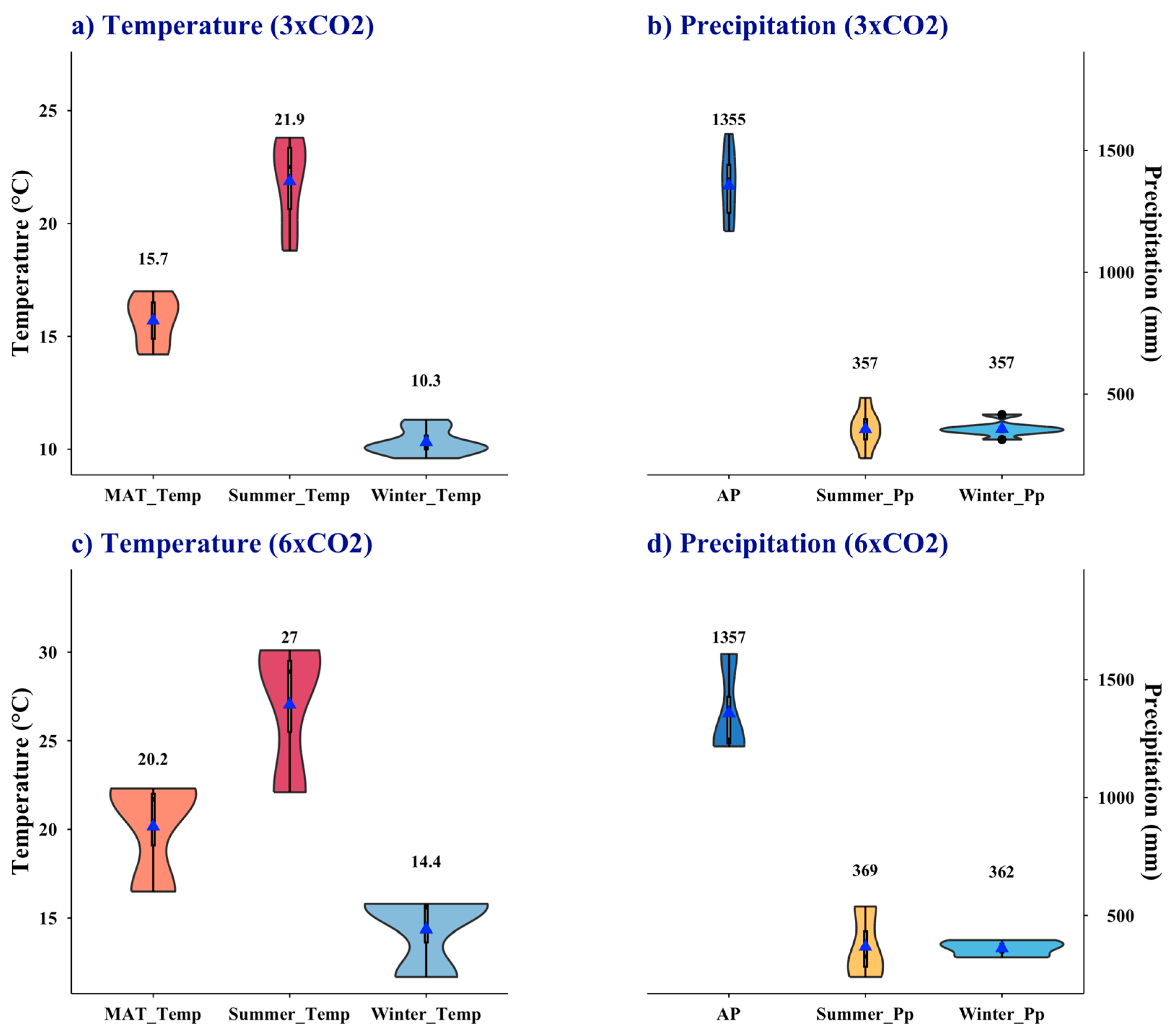
The values extracted under the 3 × CO₂ and 6 × CO₂ scenarios confirm the mesothermal character of the LMF (Figure 5). Under the 3 × CO₂ models, the mean annual temperature (MAT) was 15.7 °C, with winter and summer averages of 10.3 °C and 21.9 °C, respectively (Figure 5a). Annual precipitation reached 1355 mm, with similar amounts in winter and summer (357 mm) (Figure 5b). Under the 6 × CO₂ models, MAT increased to 20.2 °C, with winter and summer averages of 14.4 °C and 27 °C, respectively (Figure 5c). Annual precipitation was 1357 mm, again showing comparable values in winter (362 mm) and summer (369 mm) (Figure 5d).

2.3. Nothofagus Ecological Niche Models and Early Eocene Suitability Across Gondwana

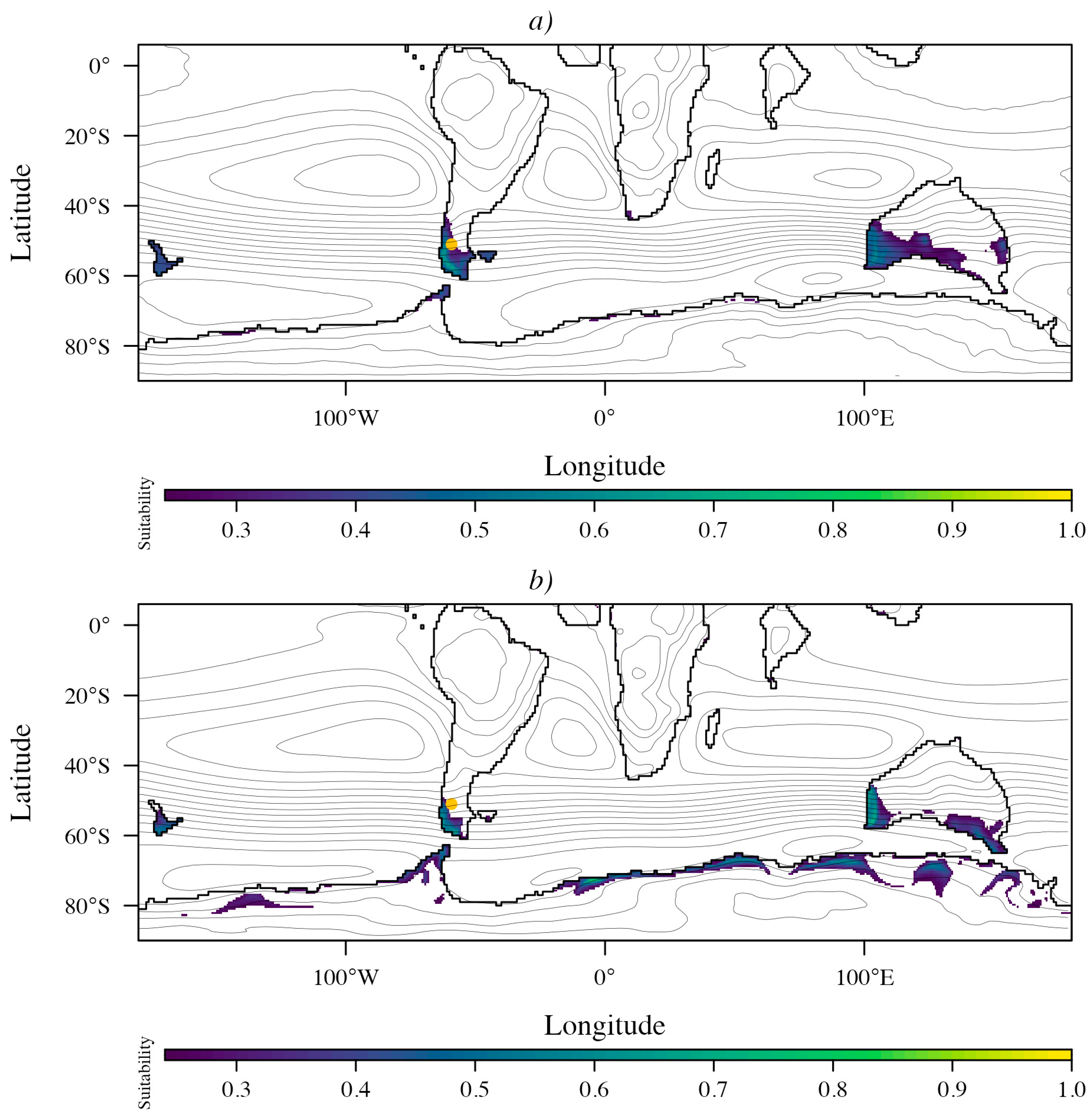
Figure 6 illustrates the ensemble-mean suitability of Nothofagus during the Eocene, projected from its current distribution under the 3 × CO₂ (Figure 6a) and 6 × CO₂ (Figure 6b) scenarios. Model performance was consistently high across DeepMIP general circulation model (GCM) specific calibrations (AUC = 0.86–0.88 and omission rate = 0.099–0.128;

Table 2. Model configuration and predictive performance across general circulation models (GCMs) and CO₂ scenarios for experiment 1. For each GCM and scenario, we report the selected Maxnet feature-class set (fc), the regularization multiplier (reg), predictive performance on the holdout test data expressed as the area under the ROC curve (AUC_test), and the omission rate on the holdout test presences at the 10th percentile training presence threshold (OR_P10). Feature classes are abbreviated as follows: lh (linear + hinge), lqh (linear + quadratic + hinge), and lqph (linear + quadratic + product + hinge). Models calibrated under 3 × CO₂ were projected to the Early Eocene under 3 × CO₂ for all GCMs, whereas CESM, GFDL, and INMCM were additionally used for 6 × CO₂ projections.

Model	Scenario	fc	reg	AUC_Test	OR P10
CESM	3 × CO2	lh	1	0.88	0.105
COSMOS	3 × CO2	lh	1	0.88	0.110
GFDL	3 × CO2	lh	1	0.86	0.099
HADCM3B	3 × CO2	lqh	1	0.88	0.128
HADCM3BL	3 × CO2	lqh	1	0.88	0.126
IPSL	3 × CO2	lh	1	0.88	0.113
MIROC	3 × CO2	lqh	1	0.87	0.118
CESM	6 × CO2	lh	1	0.88	0.105
GFDL	6 × CO2	lh	1	0.86	0.099
INMCM	6 × CO2	lqph	1	0.87	0.110

), with a regularization multiplier of 1 in all cases. Selected feature sets were dominated by linear hinge (lh), with more complex configurations (linear + quadratic + hinge (lqh) and linear + quadratic + product + hinge (lqph)) retained in a subset of models; CESM, GFDL, and INMCM were used for the 6 × CO₂ Eocene projections. The model signal was most consistently associated with hydroclimatic seasonality and thermal extremes (

Table 3. Top three predictors (permutation importance) for Experiment 1 (modern-to-Eocene transfer) across GCMs and CO₂ scenarios. Ranked predictors correspond to the three variables listed in Table 7 with the highest permutation importance in Maxnet models trained with modern Nothofagus occurrences under pre-industrial conditions and projected to Early Eocene climates. Values in parentheses indicate permutation importance within each model run.

Climate Model	Scenario	Rank 1	Rank 2	Rank 3
CESM	3 × CO2	Var6 (34)	Var4 (21)	Var18 (12)
COSMOS	3 × CO2	Var15 (29)	Var2 (24)	Var12 (16)
GFDL	3 × CO2	Var15 (40)	Var14 (38)	Var12 (18)
HADCM3B	3 × CO2	Var1 (36)	Var6 (33)	Var10 (22)
HADCM3BL	3 × CO2	Var6 (41)	Var2 (28)	Var21 (12)
IPSL	3 × CO2	Var9 (33)	Var6 (31)	Var22 (18)
MIROC	3 × CO2	Var4 (28)	Var14 (23)	Var12 (18)
CESM	6 × CO2	Var6 (34)	Var4 (21)	Var18 (12)
GFDL	6 × CO2	Var15 (40)	Var14 (38)	Var12 (18)
INMCM	6 × CO2	Var4 (45)	Var12 (22)	Var13 (21)

). JJA precipitation was the leading predictor in CESM (both 3 × CO₂ and 6 × CO₂) and in HADCM3BL (3 × CO₂) and ranked second in HADCM3B and IPSL. Temperature-related predictors were likewise recurrent, including DJF mean temperature (rank 2 in CESM; rank 1 in MIROC; and rank 1 in INMCM under 6 × CO₂), mean annual temperature (rank 1 in HADCM3B), and temperature of the warmest month (rank 1 in COSMOS, GFDL, and GFDL under 6 × CO₂). Several models also emphasized variables reflecting evaporative demand or moisture balance, such as DJF evaporation (HADCM3B), JJA EP (COSMOS, GFDL, MIROC), and EP min (IPSL), whereas orography emerged as an important constraint in some cases (notably GFDL and MIROC).

Under the 3 × CO₂ scenario, suitable conditions for Nothofagus (probability P10 > 0.24) were restricted to southwestern South America (south of ~40° S); western Australia, New Zealand, and the Antarctic Peninsula (Figure 6a). Under the 6 × CO₂ scenario, suitable areas expanded toward Antarctica but did not form a continuous corridor between South America and Australia, and only scattered, isolated patches of suitability were projected across the continent (Figure 6b). In both scenarios, the highest suitability was largely concentrated within regions influenced by the Southern Hemisphere westerlies (Figure 6).

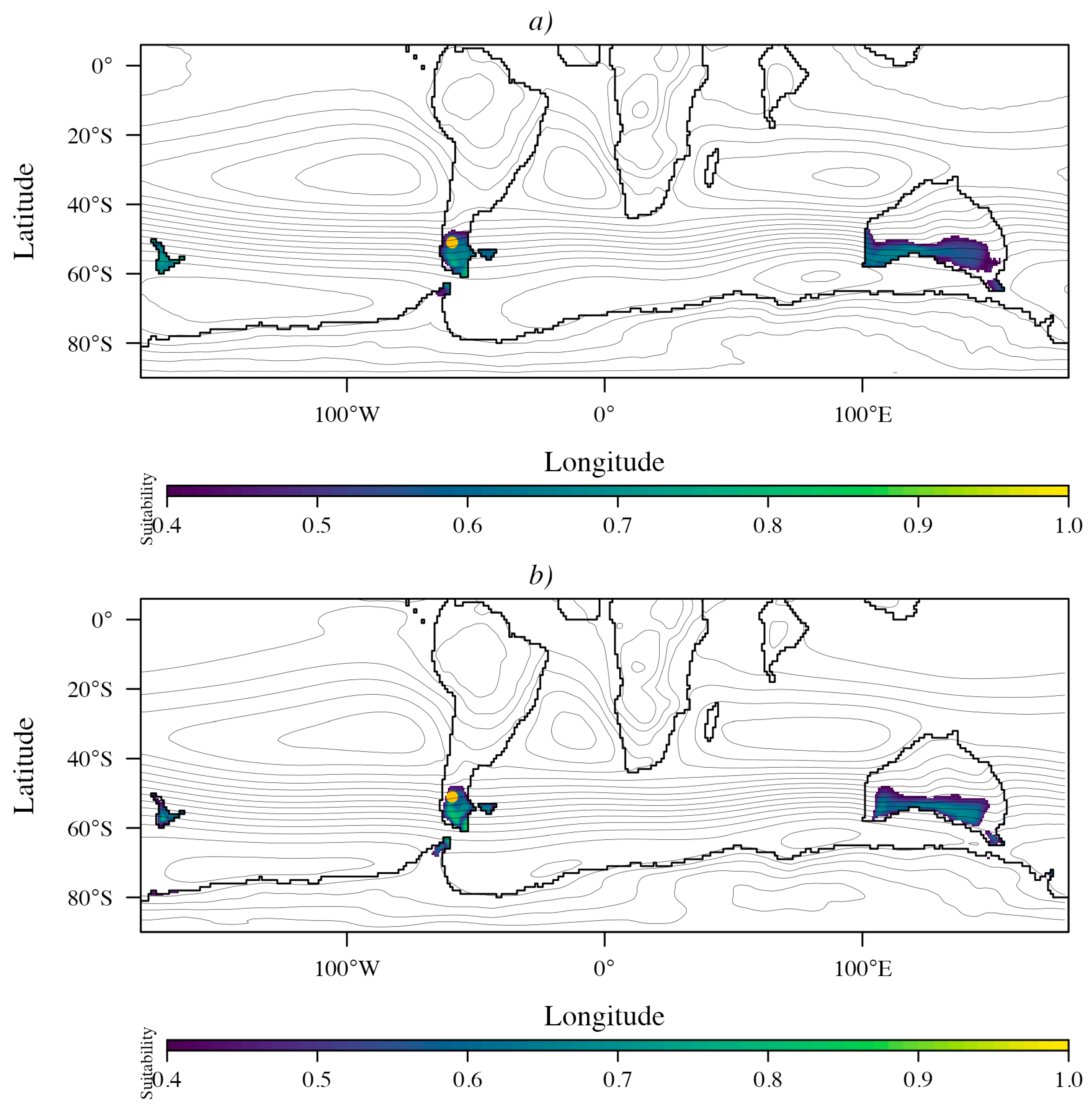
Figure 7 illustrates the ensemble-mean suitability of Nothofagus during the Eocene, projected from its Eocene occurrence records under the 3 × CO₂ (Figure 7a) and 6 × CO₂ (Figure 7b) scenarios. Model performance was consistently high across DeepMIP general circulation model (GCM)–specific calibrations (AUC = 0.89–0.98 and omission rate = 0.091–0.182;

Table 4. Model configuration and predictive performance across general circulation models (GCMs) and CO₂ scenarios for experiment 2. For each GCM and scenario, we report the selected Maxnet feature-class set (fc), the regularization multiplier (reg), and predictive performance on the holdout test data expressed as the area under the ROC curve (AUC_test). We also report the omission rate at the 10th percentile training presence threshold (OR_P10), evaluated on all available Eocene presence records (n = 11); because of the small sample size, omission rates are necessarily discrete (multiples of 1/11). Feature classes are abbreviated as follows: lh (linear + hinge), lqh (linear + quadratic + hinge), and lqph (linear + quadratic + product + hinge). Models calibrated under 3 × CO₂ were projected to the Early Eocene under 3 × CO₂ for all GCMs, whereas CESM, GFDL, and INMCM were additionally used for 6 × CO₂ projections.

Model	Scenario	fc	reg	AUC_Test	OR_P10
CESM	3 × CO2	lh	1	0.91	0.182
COSMOS	3 × CO2	l	2.5	0.93	0.182
GFDL	3 × CO2	lq	3	0.98	0.091
HADCM3B	3 × CO2	lqph	1	0.92	0.182
HADCM3BL	3 × CO2	lqph	1	0.93	0.182
IPSL	3 × CO2	lh	1	0.89	0.182
MIROC	3 × CO2	lq	1	0.95	0.182
CESM	6 × CO2	lh	1	0.91	0.182
GFDL	6 × CO2	lq	3	0.98	0.091
INMCM	6 × CO2	lq	1.5	0.87	0.182

), with modest variation in model complexity reflected by the selected feature classes (l, lh, lq, lqph) and regularization multipliers (1–3; Table 4). Variable-importance rankings (

Table 5. Top three predictors (permutation importance) for Experiment 2 (Eocene-to-Eocene calibration) across GCMs and CO₂ scenarios. Ranked predictors correspond to the three variables listed in Table 2 with the highest permutation importance in Maxnet models trained with modern Nothofagus occurrences under pre-industrial conditions and projected to Early Eocene climates. Values in parentheses indicate permutation importance within each model run.

Climate Model	Scenario	Rank 1	Rank 2	Rank 3
CESM	3 × CO2	Var4 (70)	Var14 (8)	Var22 (7)
COSMOS	3 × CO2	Var4 (72)	Var14 (11)	Var8 (9)
GFDL	3 × CO2	Var15 (45)	Var14 (22)	Var21 (21)
HADCM3B	3 × CO2	Var14 (48)	Var1 (21)	Var9 (12)
HADCM3BL	3 × CO2	Var14 (38)	Var4 (20)	Var8 (12)
IPSL	3 × CO2	Var6 (61)	Var19 (7)	Var13 (7)
MIROC	3 × CO2	Var14 (33)	Var2 (22)	Var3 (20)
CESM	6 × CO2	Var4 (70)	Var14 (8)	Var22 (7)
GFDL	6 × CO2	Var15 (45)	Var14 (22)	Var21 (21)
INMCM	6 × CO2	Var2 (45)	Var3 (22)	Var21 (21)

) showed that the dominant predictors shifted toward stronger topographic and seasonal-temperature control across multiple GCMs. DJF mean temperature clearly dominated CESM and COSMOS (both scenarios), while orography ranked first in HADCM3B, HADCM3BL, and MIROC (3 × CO₂) and ranked second in several other GCMs, indicating an increased sensitivity to physiographic structure in the fossil-calibrated reconstructions. GFDL remained primarily driven by the temperature of the warmest month (rank 1 in both scenarios), with orography and EP max consistently ranking second and third, respectively. In IPSL, JJA precipitation was overwhelmingly dominant (rank 1), whereas INMCM under 6 × CO₂ showed a distinct response in which temperature range (Tmax–Tmin) and JJA mean temperature were the leading predictors, again coupled with EP max.

Under the 3 × CO₂ scenario, suitability (probability P10 > 0.5) was concentrated within the westerlies-influenced belt south of ~40° S, including southern South America, southern Australia, New Zealand, and the Antarctic Peninsula (Figure 7a). Under the 6 × CO₂ scenario, suitable areas expanded within the Antarctic Peninsula and included an isolated region in eastern Antarctica; however, Antarctica did not form a continuous corridor between South America and Australia, and only scattered, isolated patches of suitability were projected across the continent (Figure 7b).

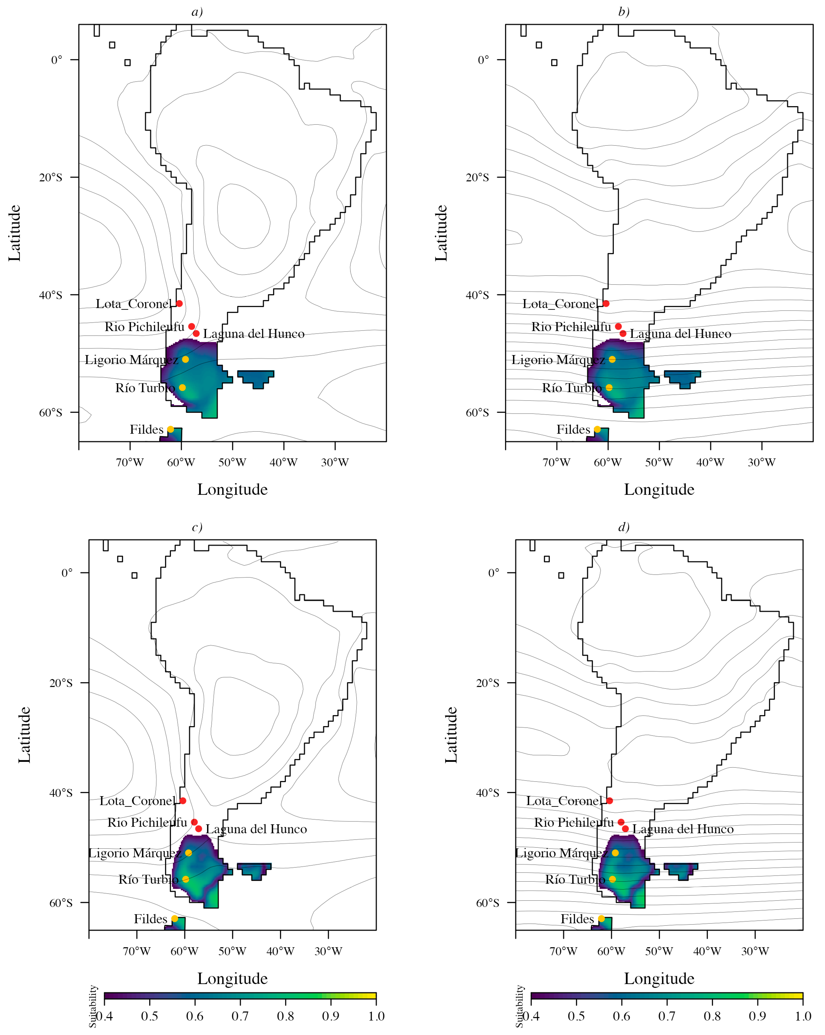
Figure 8 illustrates the probability of Nothofagus occurrence in South America and the Antarctic Peninsula in relation to the pressure system during winter (Figure 8a,c) and summer (Figure 8b,d). Panels a and b correspond to the mean of the 3 × CO₂ models, while panels c and d correspond to the mean of the 6 × CO₂ models. Nothofagus Eocene distribution is associated mainly with the westerlies belt, with a northern limit restricted by the presence of the South American anticyclone during the summertime. This transition area will lie between South America’s subtropical and temperate climates and will separate the Eocene floras with and without Nothofagus.

3. Discussion

The mid-latitudes south of ~40° S during the Eocene was predominantly mesothermal (Figure 3 and Figure 4), supporting highly diverse floras. Laguna del Hunco, among the most diverse Eocene macrofloras, is linked to EECO [16]. Paleoclimate estimates for this flora indicate mesothermal conditions, with a mean annual temperature of 16.6 °C and annual precipitation of 1140 mm. Similarly, high diversity is documented in the Rio Turbio microflora [8,16,33], with mean annual temperatures of ~16 °C and annual precipitation of 1540 mm [18,21]. For Ligorio Márquez flora, DeepMIP-based values are ~3.4 °C cooler under 3 × CO₂ (MAT = 15.7 °C; range: 14.2–17.0 °C; Figure 5a) than previous estimates (19.1 °C; range: 17.2–20.9 °C) reported by Hinojosa et al. [28] and Quattrocchio et al. [21]. By contrast, the earlier estimates are more consistent with the 6 × CO₂ scenario (20.2 °C; range: 16.5–22.3 °C), although all values remain within the mesothermal range expected for the Early Eocene in this region.

Our diversity findings from the LMF (Figure 1 and Figure 2 and Figure S1) are consistent with the influence of the Paleocene/Eocene–Early Eocene Hothouse climate on southern South American biodiversity, with species richness comparable to that of the most diverse Patagonian microfloras reported to date [33]. In contrast, the LMF appears more diverse than the Paleocene–Early Eocene microfloras of Chorrillo Chico and Agua Fresca Formations, as indicated by rarefaction analyses (Figure 3). This disparity may be partly explained by taphonomic processes. Carrillo-Berumen et al. [34] reported that Chorrillo Chico and Agua Fresca exhibit high richness and abundance of sporomorphs associated with fluvio-deltaic systems (suggesting proximity to a continental source), whereas the consistent presence of Impagidinium dinocysts indicates deposition in a distal marine setting under hyperpycnal conditions. Such depositional differences could affect both preservation and the effective area sampled by palynological assemblages, thereby influencing apparent richness. Additionally, potential age differences among the Formations may also contribute to the observed offset, because even modest temporal differences within the Paleocene–Eocene interval could capture distinct climatic or ecological phases.

The high palynofloral diversity documented here for the LMF contrasts with previous reports [31,32] not only in the number of taxa and the absence of Nothofagus in the pollen rain, but also in the low similarity between studies (see Figure S2, Supporting Information). This discrepancy has been attributed to the presence of two distinct microfloras, an older assemblage lacking Nothofagus and a younger one in which Nothofagus is present, deposited under changing climatic conditions [26]. Alternatively, the observed differences may reflect variations in sampling effort or taphonomic biases rather than climate [27]. The presence of Nothofagus in the macroflora of the LMF supports this latter explanation [28].

Recently, Quattrocchio et al. [35] floristically linked the LMF with the nearby Laguna Manantiales Strata and related both with the Eocene Patagonian fossil floras, including Río Turbio Formation [8,33] and La Marcelina [36]. They classified LMF as a Gondwanan Subtropical flora, which exhibits a mixture of taxa with present-day Neotropical, Pantropical, and Australasian distributions, along with a low proportion of Antarctic elements [18,21]. This flora thrived in Patagonia during the early Eocene under subtropical conditions, with year-round precipitation [37,38,39]. From a taphonomic perspective, sporomorph assemblages in fluvial settings are commonly supplied by surface runoff, complemented by direct atmospheric deposition; therefore, comparisons among palynological assemblages derived from broadly similar fluvial depositional contexts should be comparable in their transport pathways and source-area integration, strengthening regional diversity and floristic comparisons. Accordingly, rarefaction curves are interpreted as standardized recorded palynological richness rather than direct estimates of true standing diversity, because transport, preservation, and depositional setting can bias taxonomic representation.

Eocene climate model simulations suggest that the LMF fell within a humid subtropical climate (Köppen–Geiger Cfa) under both 3 × CO₂ and 6 × CO₂ scenarios, characterized by the absence of a dry season and hot summers, with the warmest month exceeding 22 °C. Under the 3 × CO₂ scenario, the Cfa climate extended from approximately 40° S to 50–55° S, where it transitioned poleward into the temperate oceanic/subtropical highland climate (Cfb; Figure 3c). The Cfb climate is characterized by a coldest month averaging above 0 °C, all months with average temperatures below 22 °C, and no significant seasonal differences in precipitation. During the Eocene under 3 × CO₂ scenario, Cfb conditions dominated the southernmost latitudes of South America and the Antarctic Peninsula (Figure 3c). At present, the Cfa climate occurs in northeastern Argentina and southern Brazil, while the Cfb climate is found in southern Chile and western Argentina south of 38° S; in the northeastern Andes north of ~18° S; in southern Brazil at ~23–29° S; and along the eastern margin of Argentina at ~36–38° S [40]. This disjunct distribution of Cfb is due to the presence of extensive arid climates (Köppen’s B type) that cross the Andes along the Arid Diagonal of South America [41]. Notably, the Cfa climate would have covered the entire region south of ~40° S during the Eocene under the 6 × CO₂ scenario (Figure 4c).

According to our hypothesis, humid temperate climates without a dry season (Köppen–Geiger Cf, within the broader mesothermal C group) are suitable for Gondwanan lineages [28]. Our niche modeling based on modern occurrence records (Figure 1) and Eocene projections under 3 × CO₂ and 6 × CO₂ scenarios (Figure 6) indicates a high probability of Nothofagus occurrence within the region influenced by the humid Southern Hemisphere westerlies, although there are differences between scenarios. Under the 3 × CO₂ scenario, suitable conditions for Nothofagus were largely restricted to southwestern South America (south of ~40° S), western Australia, and New Zealand, whereas under the 6 × CO₂ scenario, suitability expanded into Antarctica; however, projections across the continent were discontinuous and largely confined to scattered, isolated patches (Figure 6b).

Additional differences and similarities emerged when fossil occurrences were used to reconstruct the Eocene niche of Nothofagus. As in the projections based on modern records, suitability under both the 3 × CO₂ and 6 × CO₂ scenarios is concentrated within the westerlies-influenced belt south of ~40° S, encompassing southern South America, southern Australia, and New Zealand. However, under the 6 × CO₂ scenario, areas of high suitability were largely absent (Figure 7). Consistent with expectations, the Antarctic Peninsula appears to have provided suitable conditions for Nothofagus during the Eocene. Importantly, the taxa is also documented by macrofossils from the Antarctic Peninsula into the early Miocene [42], indicating long-term persistence and highlighting Antarctica’s key role in the evolutionary history of the genus. The southern South America–Antarctic Peninsula region has been proposed as a source area for the migration of Nothofagus (and other Gondwana lineages) to Australia since the latest Cretaceous–early Cenozoic times, and dispersal routes must have involved Antarctica [43].

Our Eocene niche models for Nothofagus indicate low climatic suitability across much of Antarctica, suggesting that a trans-Antarctic route would have been challenging and that connectivity may have been spatially restricted and/or intermittent (Figure 7 and Figure 8). In contrast, high suitability in New Zealand and Tasmania (Figure 7) points to these regions as potential areas of persistence and diversification within eastern Gondwana, consistent with scenarios involving rare long-distance dispersal from the southern South America–Antarctic Peninsula region. Such a mechanism could help explain the Eocene divergence between the Nothofagus subgenus Nothofagus (currently restricted to South America) and Brassospora (restricted to Papua New Guinea and New Caledonia), dated at ~42.2 Ma (56.4–31.5 Ma; [44]). Additional support for an Antarctic component in this history comes from newly reported Nothofagus fossil evidence interpreted as affiliated with the Brassospora lineage from Early Eocene deposits of the La Meseta Formation, Antarctica [45].

Interpreting the mismatch between the modern-to-Eocene transfer models (Experiment 1) and the fossil-calibrated projections (Experiment 2) requires distinguishing climatic suitability from realized occupancy and considering whether climatic niches were conserved through time [46,47]. Our phylogenetic analyses support climatic niche conservatism in Nothofagus, but with pronounced lineage-level differentiation, such that Eocene occurrences occupy warmer climatic space closer to that of extant Brassospora than to the modern South American lineages that dominate the present-day realized niche [28]. Consequently, projections based on modern South American occurrences may underrepresent suitability in warmer Eocene environments, whereas fossil calibrated models better capture the climatic niche expressed by Eocene populations/lineages. This lineage structure interacts with geography: Köppen–Geiger reconstructions indicate that Antarctica was dominated during the Early Eocene by continental (D) climates (including Dsa and colder variants), with humid temperate Cf climates were spatially restricted (see Figure S3, Supporting Information), consistent with fragmented Antarctic suitability under 6 × CO₂ (and largely absent under 3 × CO₂) rather than a continuous corridor (Figure 6 and Figure 7). Finally, limited effective dispersal and colonization lags could have prevented continuous occupancy even where suitability was locally high [48,49], reinforcing the inference of restricted and intermittent connectivity across Antarctica during peak hothouse conditions.

An alternative, non-exclusive interpretation is that Nothofagus occupied only a limited subset of Antarctic environments during the Early Eocene, potentially cooler inland settings and/or higher elevations, rather than being widespread across the continent [7,9,50]. This view is consistent with the offshore early Eocene (53.9–51.9 Ma) pollen record from Wilkes Land (Site U1356; Figure S4, Supporting Information), which indicates mesothermal, stratified forests including Bombacoideae, Strasburgeria, palms, and Proteaceae, and implies strong spatial climatic gradients that could have restricted temperate rainforest elements to cooler refugial areas [7,9]. Notably, Wilkes Land and the LMF exhibit comparable diversity under equivalent sampling effort (Figure S5, Supporting Information) and similar mesothermal reconstructions (e.g., MAT = 16 ± 3 °C; AP = 132 ± 55 cm) for Wilkes Land [9]. However, our niche models (Figure 6 and Figure 7) suggest that many inland and/or higher-elevation Antarctic settings remained of low suitability for Nothofagus during this hothouse interval, whereas suitability along Antarctica was discontinuous and largely confined to discrete coastal sectors. Under 6 × CO₂ scenario, both experiments recover a coastal window of suitability in the Wilkes Land sector (Figure 6b and Figure 7b; Figure S4, Supporting Information).

Beyond Antarctica, our projections also identify suitable habitats in Australia, including portions of the hinterland and selected coastal regions (Figure 6 and Figure 7), consistent with earlier paleobotanical syntheses [50]. The apparent scarcity or absence of Nothofagus evidence in some of these climatically suitable Australian regions during the hothouse interval may therefore reflect dispersal limitation, whereby taxa fail to occupy environmentally suitable areas because propagules do not reach them [51]. Targeted discovery of additional Nothofagus megafossils (e.g., leaves, wood, or reproductive structures) from Australia or East Antarctica would provide critical constraints on whether these regions hosted undocumented populations and would help discriminate among competing scenarios of connectivity, range fragmentation, and dispersal limitation during the Early Eocene.

In South America, our niche modeling indicates that both Cfa and Cfb climates were suitable for Nothofagus during the Eocene (Figure 3 and Figure 4). However, according to the fossil record, floras north of LMF (Figure 8), such as those at Laguna del Hunco, lack megafossils of Nothofagus. This pattern is also observed in other Eocene floras, such as Río Pichileufú and Lota-Coronel [15,52]. These have historically been classified as a distinct floristic unit known as Mixed Floras without Nothofagus [15,22,23,53]. It is not clear why Nothofagus doesn’t reach lower latitudes, and this may be attributed to rapid climatic or landscape changes occurring over short timescales [54]. The absence of Nothofagus in the Laguna del Hunco flora, dated at 51.91 ± 0.22 Ma during the Early Eocene Climatic Optimum, may be explained by climatic differences relative to the slightly older Ligorio Márquez flora (~53 Ma). However, the absence of this taxon in the Pampa Jones flora, located approximately 1.4° north of Laguna del Hunco and dated at 54.24 ± 0.45/53.64 ± 0.35 Ma [54], suggests that regional climatic differences, rather than temporal ones, may account for its distribution.

Figure 8 compares the mean sea-level pressure during the austral summer (Figure 8a) and winter (Figure 8b). The fossil floras located north of LMF were under the influence of an anticyclonic system during the summer, which likely acted as an environmental filter, limiting the northward distribution of Nothofagus during the Eocene. Hinojosa et al. [28] evaluated the phylogenetic signal of environmental variables related to temperature and precipitation. Their findings indicate that Nothofagus is highly sensitive to precipitation changes, consistent with a stabilizing selection model within an Ornstein-Uhlenbeck evolutionary framework. As a result, the annual variation in anticyclonic influence at mid-latitudes in South America likely acted as an effective environmental filter for Nothofagus during the Eocene and as a stabilizing selection force throughout the Cenozoic. The modern distribution of Nothofagus in Mediterranean climates in South America supports the hypothesis of stabilizing selection by the annual precipitation regime influencing the genus distribution in this region. A plausible trait-based mechanism underlying precipitation-linked filtering in Nothofagus is recruitment limitation under seasonal water deficit, as manipulative experiments show that seedling survival, growth, and eco-physiological performance are strongly constrained by water shortage and drought associated with warming [55,56].

The Eocene Cfa mesothermal climate, occurring at mid-latitudes in South America, has been proposed as a source of diversity for tropical regions [28]. Several taxa exhibit a disjunct distribution between temperate and tropical latitudes today, reflecting ancestral mesothermal climatic niches that shifted from high or mid-latitudes toward lower latitudes due to climatic and tectonic changes [28,41,57,58,59,60]. This suggests that modern areas under Cfa mesothermal climates in South America may harbor ancient lineages rooted in the early Cenozoic paleofloras of southern South America, as supported by molecular evidence [61].

To explore the paleoclimatic context of our fossil assemblages, we employed multiple general circulation models (GCMs) simulating conditions for the Hothouse interval [1,29]. These models provide spatially explicit reconstructions of key climate variables and allow for comparisons across regions, even in areas with limited fossil data. However, their coarse resolution and reliance on uncertain boundary conditions present limitations, particularly for local-scale interpretations [62]. By using an ensemble of models, we aim to capture a range of plausible scenarios, while emphasizing that model-based interpretations must be integrated with independent geological and paleontological evidence, as done in this study.

4. Materials and Methods

4.1. Rarefied Richness Across Eocene Hothouse Assemblages

To compare the diversity during the hothouse period in southern South America between Ligorio Marquez and other floras, we built a dataset with the abundance of morphospecies from Ligorio Marquez Formation (LMF), Laguna del Hunco (LH), Chorrillo Chico Formation (CCF), Agua Fresca Formation (AF), Lower Rio Turbio (LRT), and Upper Rio Turbio (URT).

The Ligorio Márquez Formation (LMF) crops out in Chilean Patagonia and preserves fossil-bearing continental deposits that record early Paleogene environments in the region. The age of the LMF is constrained by radiometric dating and palynological evidence. U–Pb zircon ages from stratigraphically ascending levels (57.3 ± 2.7 Ma, 53.7 ± 2.9 Ma, and 50.5 ± 2.5 Ma) provide maximum depositional ages spanning the late Paleocene (Thanetian) to Early Eocene (Ypresian), and constrain the upper part of the Formation to the Early Eocene [63]. These ages are consistent with K–Ar and ⁴⁰Ar/³⁹Ar dates reported for the overlying Basaltos Inferiores Meseta Chile Chico (BIMCC) unit [27,64]. Taken together, the available geochronological constraints indicate that the fossiliferous interval yielding the LMF flora most plausibly falls within the Early Eocene (Ypresian).

The age of the flora has been approached by different authors. Suárez et al. [26] and Troncoso et al. [31] reported 19 leaf taxa, mainly associated with Lauraceae, and 12 spore and pollen taxa, highlighting the absence of Nothofagus. They compared their findings with the Chilean fossil flora of Lota-Coronel [52] and suggested a similar age. The Lota-Coronal flora is deposited in the coal-bearing strata of the Curanilahue Formation in Central Chile and has been assigned to the Upper Paleocene-Early Eocene (but see [65]). In addition, the occurrence of Malvacipollis diversus and Retitricolporites medius supports an early Eocene age for the LMF flora [28,35,66] (see Supplementary Information for discussion).

The LMF data were collected from 35 horizons and sampled in 50 m sections. From the base to the top, 23 samples were taken from deposits of floodplain and sandstones (located in the first 20 m of the section), eight samples from coal lines and siltstones (located between 20 and 40 m), and the remaining four samples from sandstones at the top section (between 40 and 50 m, see Figure S6 Supporting Information). The palynological samples were prepared by the standard procedure of digesting the sample in HF and HCl acids, separating organic matter by heavy liquids, and oxidizing [67]. A complete oxidized slide per sample was scanned with a 20X Zeiss (Oberkochen, Germany) plan apochromatic objective, and 300 palynomorphs per slide were counted when possible [66]. The age of LMF is Early Eocene [28,63,64,66].

The LH microflora was reported by Barreda et al. [68]. The samples were collected from seven stratigraphic levels in the Huitrera Formation, in Chubut, Argentina. These outcrops are the remains of a fossil caldera lake in the Middle Chubut River. 56 spore and pollen species and 28 plant families were recovered. The age of LH is Early Eocene [14,16].

The Chorrillo Chico Formation and Agua Fresca Formation microflora were reported by Carrillo-Berumen et al. [34]. These Formations are exposed in a Paleogene section of Punta Prat, Chile, in the southern Magallanes-Austral Basin. Both units contain a palynological assemblage composed of marine and continental palynomorphs, indicative of a marine depositional environment with terrigenous input. Chorrillo Chico has 56 pollen and spore species, with 16 angiosperms, 12 gymnosperms, and 28 spores. The age of CC is Paleocene (Thanetian). Agua Fresca has 50 pollen and spore species, with 14 angiosperms, 12 gymnosperms, and 24 spores. The age of AF is Early Eocene [69].

The Rio Turbio Formation microflora was reported by Fernandez et al. [8]. Samples collected from the Lower section of the Formation have 108 pollen and spore species, with 68 Angiosperm, 10 Gymnosperm, and 30 spores. The Upper section has 101 pollen and spore species, with 67 Angiosperm, 8 Gymnosperm, and 26 spores. The age of RTF is constrained as the mid-late Eocene (~47–34 Myr [70]).

We evaluated differences in species richness among fossil microfloral assemblages using rarefaction/extrapolation [71] curves in iNEXT [72]. For formal inference, we compared rarefied species richness (q = 0) at a common number of individuals, m₀, defined as the minimum observed total abundance among assemblages retained for comparison (thus avoiding extrapolation). Assemblages with very low total abundance were excluded using an explicit threshold rule, N < max [1000, 0.5 × N2nd_smallest], where N2nd_smallest is the second-smallest observed sample size across assemblages. All pairwise tests were then conducted among the remaining sites using the same m₀. For each assemblage, we generated 200 bootstrap replicates via multinomial resampling (total N fixed), reran iNEXT for each replicate, and extracted S_X(m₀) (or the nearest reported sample size). Pairwise differences were computed as Δ = S_A (m₀) − S_B (m₀), where S_X (m₀) is the rarefied richness of assemblage X at m₀; Δ > 0 indicates higher richness in A. We report bootstrap 95% confidence intervals and two-sided bootstrap p-values, with Bonferroni correction for multiple comparisons.

4.2. Mesothermal, Humid Conditions at LMF in 3× and 6× pCO₂ DeepMIP Simulations

To assess the mesothermal paleoclimate accuracy of the LMF paleoclimate, previously published by Hinojosa et al. [28], we compared it with the estimate obtained by the Deep-Time Model Intercomparison Project (DeepMIP, Lunt et al. [29]). We used simulations of preindustrial control and Early Eocene simulations at CO₂ concentrations of approximately 800 ppm (×3 pre-industrial levels) in seven models and 1600 ppm (×6 pre-industrial levels) in three models (

Table 6. Global circulation models from the Deep-Time Model Intercomparison Project (DeepMIP-Eocene, Lunt, et al. [29]).

Model	Short Name	CO2 Experiment	Simulation Reference
CESM1.2_CAM5	CESM	×3, ×6	[75]
COSMOS-landveg_r2413	COSMOS	×3	[29]
GFDL_CM2.1	GFDL	×3, ×6	[29]
HadCM3B_M2.1aN	HadCM3	×3	[29]
HadCM3B_L M2.1aN	HadCM3	×3	[29]
INM-CM4-8	INMCM	×6	[29]
IPSLCM5A2	IPSL	×3	[76]
MIROC4m	MIROC	×3	[29]

). DeepMIP Eocene experiments are designed to represent Early Eocene boundary conditions rather than a single discrete time slice; therefore, we use 3 × CO₂ and 6 × CO₂ as bracketing forcings that span plausible atmospheric CO₂ levels for the LMF age range constrained by U–Pb maximum depositional ages (~54–53 Ma) and for comparison with floras close to peak EECO conditions. Accordingly, 3 × CO₂ provides a conservative baseline, whereas 6 × CO₂ approximates peak hothouse forcing. According to Lunt et al. [29], the paleogeography, vegetation, and river routing for the Eocene simulations correspond to those of Herold et al. [73]. The solar constant, orbital configuration, and non-CO2 greenhouse gas concentrations were set to preindustrial values. Soil properties were set to homogeneous global mean values derived from the preindustrial simulation, and there were no continental ice sheets in the Eocene simulations. For details on each model, please refer to Lunt and collaborators [29,74].

From each Early Eocene model in Table 6, we obtained 22 raster environmental variables related to temperature, precipitation, evapotranspiration, hydric balance (evapotranspiration minus precipitation), and orography. Because the DeepMIP models have varying native spatial resolutions, all fields were harmonized by reprojection onto a common 5′ × 5′ global grid using the coordinate reference system ‘+proj = longlat + datum = WGS84’ (extent: −180° to 180° longitude and −90° to 90° latitude). Values on the target grid were computed using the ‘bilinear’ interpolation method from the Terra R package. We emphasize that this procedure is a grid-matching interpolation for comparability and mapping, rather than a physical (dynamical or statistical) downscaling; therefore, it does not generate new fine-scale climate information or resolve microclimates or local orographic effects in complex topography. Accordingly, site-level values should be interpreted as regional approximations. A total of 22 raster-based environmental variables were obtained, including data on temperature, precipitation, evapotranspiration, hydric balance (evapotranspiration minus precipitation), and orographic conditions during the Eocene (

Table 7. Twenty-two environmental variables derived from the ensemble mean model used for niche modeling.

Variable Name	Variable
Var1	Mean annual temperature (°K)
Var2	Range Temperature (temp max − temp min) × 10 (°K)
Var3	JJA mean temp (°K)
Var4	DJF mean temp (°K)
Var5	Annual precipitation (mm)
Var6	JJA precipitation (mm)
Var7	DJF precipitation (mm)
Var8	Annual evaporation (mm)
Var9	JJA evaporation (mm)
Var10	DJF evaporation (mm)
Var11	Annual Hydric Balance (EP, Bio8-Bio5) (mm)
Var12	JJA EP (mm)
Var13	DJF EP (mm)
Var14	Orography (m.a.s.l)
Var15	Temperature of the warmest month (°K)
Var16	Temperature of the coolest month (°K)
Var17	Precipitation of the wetter month (mm)
Var18	Precipitation of the driest month (mm)
Var19	Evaporation of the warmest month (mm)
Var20	Evaporation of the coolest month (mm)
Var21	EP max (Var19-Var17) (mm)
Var22	EP min (Var20-Var18) (mm)

). The paleo-coordinates of the LMF were plotted onto these rasters, and values for each environmental variable were extracted using the ‘extract’ function of the terra R package [77]. Finally, an ensemble-mean model was calculated for both the 3 × CO₂ and 6 × CO₂ experiments. Using reconstructed monthly paleoclimate rasters of temperature and precipitation, we classified the Early Eocene climate of South America into Köppen–Geiger climate types [40], and the LMF, along with other Eocene floras, was classified accordingly.

4.3. Nothofagus Ecological Niche Models and Early Eocene Suitability Across Gondwana

We performed ecological niche modeling [78] to estimate the potential distribution of Nothofagus during the Early Eocene under two complementary experiments. In Experiment 1 (modern-to-Eocene transfer), models were calibrated using the modern distribution of Nothofagus under pre-industrial (PI) climatic conditions and subsequently projected onto Early Eocene climates across Gondwana (South America, Antarctica, Australia, and New Zealand) under both 3 × CO₂ and 6 × CO₂ scenarios. Modern occurrences were spatially thinned prior to modeling, and models were fitted separately for each GCM listed in Table 6 using the corresponding environmental predictors (Table 7). For each GCM, we defined the calibration region as a 450 km buffer around the thinned occurrences, masked the PI environmental stack to this domain, and sampled 15,000 random background points within it. We selected 450 km as a pragmatic extent to approximate the accessible area (M) for background sampling and to ensure that the calibration domain encompassed the main geographic components of the native Nothofagus range across Gondwana, including New Zealand, New Caledonia, and Papua–New Guinea, thereby avoiding artificial truncation of the accessible environmental background. Predictor redundancy was reduced by removing near-zero-variance variables and filtering multicollinearity using Spearman correlations computed from 10,000 randomly sampled raster cells; correlated predictors were removed using a threshold of r ≥ 0.80. Model complexity was tuned using k-fold cross-validation and a grid search over feature-class combinations and regularization multipliers (1–3, step 0.5), selecting the configuration that maximized AUC and minimized the omission rate on holdout test presences at the 10th-percentile training presence threshold (OR_P10), and favoring simpler feature sets when performance differences were negligible. Final models were refitted with the selected settings and projected using cloglog output.

In Experiment 2 (Eocene-to-Eocene calibration), we reconstructed the Eocene niche directly from fossil evidence by calibrating models with Eocene Nothofagus occurrences (in paleocoordinates) and projecting within the Early Eocene climatic space for each CO₂ scenario and GCM (Table 1). Because fossil occurrences are geographically restricted, we defined the calibration region using a fixed bounding box enclosing the fossil localities, cropped the Early Eocene predictor stack to this region, and sampled 15,000 random background points within the cropped domain. The same workflow for predictor screening (near-zero-variance removal and Spearman correlation filtering at r ≥ 0.80), hyperparameter tuning (cross-validation and grid search using AUC, we also report OR_P10 evaluated on all Eocene presences (n = 11), which yields discrete values (multiples of 1/11)), and prediction settings (cloglog output) was applied. To quantify uncertainty in both experiments, we implemented 10 bootstrap replicates per GCM and scenario by resampling presences with replacement while keeping background points constant, and summarized replicate projections as ensemble-mean rasters. Models were fitted under the maximum-entropy framework [79,80] using SDMtune [81], with models trained via the Maxnet method implemented in the R package maxnet [82].

To summarize high-suitability areas from these presence-only models, we used the 10th percentile training presence threshold (P10) as a reference for visualizing the continuous cloglog suitability surfaces in Experiments 1 and 2 (i.e., color scales were set to begin near P10 to emphasize the suitability range supported by training presences). P10 is a commonly used MaxEnt/Maxnet threshold that is comparatively robust to a small number of low-suitability outlier occurrences and provides a pragmatic compromise between omission error and overprediction when interpreting suitability surfaces [83,84]. Because P10 values differed between the two modeling settings, we computed experiment-specific P10 thresholds for each GCM and CO₂ scenario, using the mean P10 across bootstrap replicates.

Finally, we used the bioclimatic thermal regime proposed by Nix [4]: megathermal climate (MAT ≥ 22 °C, MAP > 549 mm); mesothermal climate (MAT ≥ 14–22 °C, MAP > 549 mm); and microthermal climate (MAT < 14 °C, MAP 719–3000 mm) and Köppen -Geiger climate classification [40]. This Classification defines five major climate types based on temperature and precipitation thresholds and was implemented in R using a translation of the Beck et al. [85] algorithm.

5. Conclusions

The Ligorio Márquez Formation hosted a highly diverse palynoflora comparable to other diversity-rich Eocene assemblages in southern South America, and it developed under mesothermal, humid Cf conditions.

Niche-model projections indicate that climatically suitable habitats for Nothofagus were broadly concentrated in western Gondwana (southern South America, the Antarctic Peninsula, Australia, and New Zealand). In contrast, suitability across Antarctica was discontinuous, suggesting a limited role for Antarctica as a continent-wide dispersal corridor during peak hothouse conditions; an enhanced South Pacific High likely acted as an additional environmental filter shaping South American distributions.

The Eocene prevalence of Cf-like climates implies that modern regions with comparable conditions may retain lineages with deep Cenozoic roots, while multi-model paleoclimate simulations provide a powerful interpretive framework that should be corroborated with independent geological and fossil evidence.

References

1. Westerhold, T.; Marwan, N.; Drury, A.J.; Liebrand, D.; Agnini, C.; Anagnostou, E.; Barnet, J.S.K.; Bohaty, S.M.; De Vleeschouwer, D.; Florindo, F.; et al. An astronomically dated record of Earth’s climate and its predictability over the last 66 million years. Science 2020, 369, 1383–1387. [Google Scholar] [CrossRef]
2. Zachos, J.; Pagani, M.; Sloan, L.; Thomas, E.; Billups, K. Trends, rhythms, and aberrations in global climate 65 Ma to present. Science 2001, 292, 686–693. [Google Scholar] [CrossRef]
3. Hönisch, B.; Royer, D.L.; Breecker, D.O.; Polissar, P.J.; Bowen, G.J.; Henehan, M.J.; Cui, Y.; Steinthorsdottir, M.; McElwain, J.C.; Kohn, M.J.; et al. Toward a Cenozoic history of atmospheric CO. Science 2023, 382, eadi5177. [Google Scholar] [CrossRef]
4. Nix, H. An environmental analysis of Australian rainforests. In The Rainforest Legacy, Australian National Rainforest Study; Werren, G., Kershaw, P., Eds.; Australian Government Publishing Service: Canberra, Australia, 1991; Volume 2, pp. 1–26. [Google Scholar]
5. Jaramillo, C. The evolution of extant South American tropical biomes. New Phytol. 2023, 239, 477–493. [Google Scholar] [CrossRef] [PubMed]
6. Wiens, J.J.; Donoghue, M.J. Historical biogeography, ecology and species richness. Trends Ecol. Evol. 2004, 19, 639–644. [Google Scholar] [CrossRef]
7. Pross, J.; Contreras, L.; Bijl, P.K.; Greenwood, D.R.; Bohaty, S.M.; Schouten, S.; Bendle, J.A.; Röhl, U.; Tauxe, L.; Raine, J.I.; et al. Persistent near-tropical warmth on the Antarctic continent during the early Eocene epoch. Nature 2012, 488, 73–77. [Google Scholar] [CrossRef]
8. Fernández, D.A.; Palazzesi, L.; González Estebenet, M.S.; Telleria, M.; Barreda, V.D. Impact of mid Eocene greenhouse warming on America’s southernmost floras. Commun. Biol. 2021, 4, 176. [Google Scholar] [CrossRef]
9. Contreras, L.; Pross, J.; Bijl, P.K.; Koutsodendris, A.; Raine, J.I.; van de Schootbrugge, B.; Brinkhuis, H. Early to Middle Eocene vegetation dynamics at the Wilkes Land Margin (Antarctica). Rev. Palaeobot. Palyno 2013, 197, 119–142. [Google Scholar] [CrossRef]
10. Jaramillo, C.; Rueda, M.J.; Mora, G. Cenozoic plant diversity in the Neotropics. Science 2006, 311, 1893–1896. [Google Scholar] [CrossRef] [PubMed]
11. Rull, V. Palaeofloristic and palaeovegetational changes across the Paleocene/Eocene boundary in northern South America. Rev. Palaeobot. Palyno 1999, 107, 83–95. [Google Scholar] [CrossRef]
12. Jaramillo, C.; Cardenas, A. Global Warming and Neotropical Rainforests: A Historical Perspective. Annu. Rev. Earth Planet. Sci. 2013, 41, 741–766. [Google Scholar] [CrossRef]
13. Woodburne, M.O.; Goin, F.J.; Bond, M.; Carlini, A.A.; Gelfo, J.N.; López, G.M.; Iglesias, A.; Zimicz, A.N. Paleogene Land Mammal Faunas of South America; a Response to Global Climatic Changes and Indigenous Floral Diversity. J. Mamm. Evol. 2014, 21, 1–73. [Google Scholar] [CrossRef]
14. Wilf, P.; Johnson, K.; Cúneo, R.; Smith, M.; Singer, B.; Gandolfo, M. Eocene plant diversity at Laguna del Hunco and Río Pichileufú, Patagonia, Argentina. Am. Nat. 2005, 165, 634–650. [Google Scholar] [CrossRef]
15. Rossetto-Harris, G.; Wilf, P. Reassessing floral diversity at Rio Pichileufu, earliest middle Eocene of Rio Negro, Argentina. Palaeontol. Electron. 2024, 27, a49. [Google Scholar] [CrossRef]
16. Wilf, P.; Cuneo, N.R.; Johnson, K.R.; Hicks, J.F.; Wing, S.L.; Obradovich, J.D. High plant diversity in Eocene South America: Evidence from Patagonia. Science 2003, 300, 122–125. [Google Scholar] [CrossRef]
17. Barreda, V.D.; Palazzesi, L.; Pujana, R.R.; Panti, C.; Tapia, M.J.; Fernández, D.A.; Noetinger, S. The Gondwanan heritage of the Eocene-Miocene Patagonian floras. J. S. Am. Earth Sci. 2021, 107, 103022. [Google Scholar] [CrossRef]
18. Hinojosa, L.F. Climatic and vegetational changes inferred from Cenozoic Southern South America paleoflora. Rev. Geol. Chile 2005, 32, 95–115. [Google Scholar]
19. Hinojosa, L.F.; Villagran, C. History of the southern South American forests 1. paleobotanical, geological and climatical background on Tertiary of southern South America. Rev. Chil. Hist. Nat. 1997, 70, 225–239. [Google Scholar]
20. Palazzesi, L.; Vizcaíno, S.F.; Barreda, V.D.; Cuitiño, J.; del Río, C.J.; Goin, F.; Estebenet, M.S.G.; Guler, M.V.; Gandolfo, M.A.; Kay, R.; et al. Reconstructing Cenozoic Patagonian biotas using multi-proxy fossil records. J. S. Am. Earth Sci. 2021, 112, 103513. [Google Scholar] [CrossRef]
21. Quattrocchio, M.E.; Martinez, M.A.; Hinojosa, L.F.; Jaramillo, C. Quantitative analysis of Cenozoic palynofloras from Patagonia, southern South America. Palynology 2013, 37, 246–258. [Google Scholar] [CrossRef]
22. Romero, E.J. Paleogene phytogeography and climatology of South America. Ann. Mo. Bot. Gard. 1986, 73, 449–461. [Google Scholar] [CrossRef]
23. Troncoso, A.; Romero, E.J. Evolución de las comunidades florísticas en el extremo sur de Sudamérica durante el Cenofítico. In Proceedings of the Congreso Latinoamericano de Botánica, N° 6; Fortunato, R., Bacigalupo, N., Eds.; Monographs in Systematic Botany from the Missouri Botanical Garden; Missouri Botanical Garden Press: St. Louis, MO, USA, 1998; Volume 68, pp. 149–172. [Google Scholar]
24. Hinojosa, L.F.; Armesto, J.J.; Villagran, C. Are Chilean coastal forests pre-Pleistocene relicts? Evidence from foliar physiognomy, palaeoclimate, and phytogeography. J. Biogeogr. 2006, 33, 331–341. [Google Scholar] [CrossRef]
25. Barreda, V.; Anzotegui, L.; Prieto, A.; Aceñaloza, P.; Bianchi, M.; Borromei, A.; Brea, M.; Caccavari, M.; Cuadrado, G.; Garralla, S.; et al. Diversificación y cambios de las angiospermas durante el Neógeno en Argentina. Ameghiniana 2007, 11, 173–191. [Google Scholar]
26. Suárez, M.; de la Cruz, R.; Troncoso, A. Tropical/Subtropical upper Paleocene-lower Eocene fluvial deposits in eastern central Patagonia, Chile (46°45′ S). J. S. Am. Earth Sci. 2000, 13, 527–536. [Google Scholar] [CrossRef]
27. Yabe, A.; Uemura, K.; Nishida, H. Geological notes on plant fossil localities of the Ligorio Márquez Formation, central Patagonia, Chile. In Post-Creataceus Floristic Changes in Southern Patagonia, Chile; Nishida, H., Ed.; Chuo University: Tokyo, Japan, 2006; pp. 29–35. [Google Scholar]
28. Hinojosa, L.F.; Gaxiola, A.; Perez, M.F.; Carvajal, F.; Campano, M.F.; Quattrocchio, M.; Nishida, H.; Uemura, K.; Yabe, A.; Bustamante, R.; et al. Non-congruent fossil and phylogenetic evidence on the evolution of climatic niche in the Gondwana genus Nothofagus. J. Biogeogr. 2016, 43, 555–567. [Google Scholar] [CrossRef]
29. Lunt, D.J.; Bragg, F.; Chan, W.L.; Hutchinson, D.K.; Ladant, J.B.; Morozova, P.; Niezgodzki, I.; Steinig, S.; Zhang, Z.S.; Zhu, J.; et al. DeepMIP: Model intercomparison of early Eocene climatic optimum (EECO) large-scale climate features and comparison with proxy data. Clim. Past. 2021, 17, 203–227. [Google Scholar] [CrossRef]
30. Ullah, F.; Saqib, S.; Xiong, Y.C. Integrating artificial intelligence in biodiversity conservation: Bridging classical and modern approaches. Biodivers. Conserv. 2025, 34, 45–65. [Google Scholar] [CrossRef]
31. Troncoso, A.; Suárez, M.; de la Cruz, R.; Palma-Heldt, S. Paleoflora de la Formación Ligorio Márquez (XI Región, Chile) en su localidad tipo: Sistemática, edad e implicancias paleoclimáticas. Rev. Geológica Chile 2002, 29, 113–135. [Google Scholar] [CrossRef]
32. Macphail, M.; Carpenter, R.J.; Iglesias, A.; Wilf, P. First Evidence for Wollemi Pine-type Pollen (Dilwynites: Araucariaceae) in South America. PLoS ONE 2013, 8, e69281. [Google Scholar] [CrossRef] [PubMed]
33. Fernández, D.A.; Santamarina, P.E.; Palazzesi, L.; Tellería, M.C.; Barreda, V.D. Incursion of tropically-distributed plant taxa into high latitudes during the middle Eocene warming event: Evidence from the Rio Turbio Fm, Santa Cruz, Argentina. Rev. Palaeobot. Palyno 2021, 295, 104510. [Google Scholar] [CrossRef]
34. Carrillo-Berumen, R.; Quattrocchio, M.E.; Helenes, J. Paleogene continental Palynomorphs of the formations Chorrillo Chico and Agua Fresca, Punta Prat, Magallanes, Chile. Andean Geol. 2013, 40, 539–560. [Google Scholar] [CrossRef]
35. Quattrocchio, M.; Aguero, S.; Iglesias, A.; Raigemborn, M.S. Palynostratigraphy of the early Paleogene at the Laguna Manantiales locality, southern Golfo San Jorge Basin, Argentina. Publicación Electrónica Asoc. Paleontológica Argent. 2024, 24, 108–128. [Google Scholar]
36. Noetinger, S.; Aramendía, I.; Pujana, R.R.; Massini, J.L.G.; Barreda, V.D. Eocene palynoflora from the La Marcelina Formation, Patagonia, Argentina. Bot. J. Linn. Soc. 2023, 203, 193–208. [Google Scholar] [CrossRef]
37. Compagnucci, R.H. Atmospheric circulation over Patagonia from the Jurassic to present: A review through proxy data and climatic modelling scenarios. Biol. J. Linn. Soc. 2011, 103, 229–249. [Google Scholar] [CrossRef]
38. Hinojosa, L.F.; Villagran, C. Did South. American Mixed Paleofloras evolve under thermal equability or in the absence of an effective Andean barrier during the Cenozoic? Palaeogeogr. Palaeocl 2005, 217, 1–23. [Google Scholar] [CrossRef]
39. Quattrocchio, M.; Diaz, P.E.; Agüero, L.S. The late Paleocene-Eocene interval of the Magallanes-Austral Basin (Chile-Argentina): Palynostratigraphy, paleoclimate and geochemical data. J. S. Am. Earth Sci. 2024, 133, 104706. [Google Scholar] [CrossRef]
40. Beck, H.E.; Mcvicar, T.R.; Vergopolan, N.; Berg, A.; Lutsko, N.J.; Dufour, A.; Zeng, Z.Z.; Jiang, X.; van Dijk, A.I.J.M.; Miralles, D.G. High-resolution (1 km) Köppen-Geiger maps for 1901–2099 based on constrained CMIP6 projections. Sci. Data 2023, 10, 724. [Google Scholar] [CrossRef]
41. Villagran, C.; Hinojosa, L. History of the forests of southern South America 2. phytogeographical analysis. Rev. Chil. Hist. Nat. 1997, 70, 241–267. [Google Scholar]
42. Bastias-Silva, J.; Leppe, M.; Manriquez, L.; Trevisan, C.; Fox, B.R.S.; Magiera, M.; Wilson, G.; Tavazzani, L.; Chelle-Michou, C.; Gao, L.; et al. Neogene plant macrofossils from West Antarctica reveal persistence of Nothofagaceae forests into the early Miocene. Commun. Earth Environ. 2025, 6, 965. [Google Scholar] [CrossRef]
43. Dettman, M.E.; Pocknall, D.T.; Romero, E.J.; Zamaloa, M.C. Nothofagidites Erdtman ex Potonié, 1960; a catalogue of species with notes on the paleogeographic distribution of Nothofagus Bl. (Southern beech). N. Z. Geol. Surv. Paleontol. Bull. 1990, 60, 1–79. [Google Scholar]
44. Sauquet, H.; Ho, S.Y.W.; Gandolfo, M.A.; Jordan, G.J.; Wilf, P.; Cantrill, D.J.; Bayly, M.J.; Bromham, L.; Brown, G.K.; Carpenter, R.J.; et al. Testing the Impact of Calibration on Molecular Divergence Times Using a Fossil-Rich Group: The Case of Nothofagus (Fagales). Syst. Biol. 2012, 61, 289–313. [Google Scholar] [CrossRef]
45. Cantrill, D.; Gandolfo, M.; Tosolini, A.; Korasidis, V.; Francis, J. Evidence for a warm Eocene in the southern high latitudes: A new macroflora from Seymour Island, Antarctica. In Proceedings of the XV International Palynological Congress, XI International Organization of Palaeobotany Conference, Prague, Czech Republic, 27–31 May 2024; p. 193. [Google Scholar]
46. Wiens, J.J.; Ackerly, D.D.; Allen, A.P.; Anacker, B.L.; Buckley, L.B.; Cornell, H.V.; Damschen, E.I.; Davies, T.J.; Grytnes, J.A.; Harrison, S.P.; et al. Niche conservatism as an emerging principle in ecology and conservation biology. Ecol. Lett. 2010, 13, 1310–1324. [Google Scholar] [CrossRef]
47. Wiens, J.J.; Donoghue, M.J. The Origins of the Latitudinal Diversity Gradient: Revisiting the Tropical Conservatism Hypothesis. J. Biogeogr. 2025, 52, e15172. [Google Scholar] [CrossRef]
48. Knapp, M.; Stöckler, K.; Havell, D.; Delsuc, F.; Sebastiani, F.; Lockhart, P.J. Relaxed molecular clock provides evidence for long-distance dispersal of Nothofagus (southern beech). PLoS Biol. 2005, 3, 38–43. [Google Scholar] [CrossRef]
49. Soliani, C.; Sekely, J.; Zamora-Ballesteros, C.; Heer, K.; Lepais, O.; Mondino, V.; Opgenoorth, L.; Pastorino, M.; Marchelli, P. Restricted Dispersal in the Late Successional Forest Tree Species Nothofagus Pumilio: Consequences Under Global Change. Ecol. Evol. 2025, 15, e71002. [Google Scholar] [CrossRef] [PubMed]
50. Macphail, M.; Alley, N.; Truswell, E.; Sluiter, I. Early Tertiary vegetation: Evidence from spores and pollen. In History of the Australian Vegetation: Cretaceous to Recent; Cambridge University Press: Cambridge, UK, 1994; pp. 189–261. [Google Scholar]
51. Hubbell, S.P. The Unified Neutral Theory of Biodiversity and Biogeography; Princeton University Press: Princeton, NJ, USA, 2001; p. xiv. 375p. [Google Scholar]
52. Engelhardt, H. Über Tertiärpflanzen von Chile. Abh. Senckenberg. Naturforschenden Gessellschaft 1891, 16, 629–692. [Google Scholar]
53. Romero, E.J. Paleoecología y paleofitogeografía de las tafofloras del Cenofítico de Argentina y áreas vecinas. Ameghiniana 1978, 15, 209–227. [Google Scholar]
54. Wilf, P.; Singer, B.S.; Zamaloa, M.D.; Johnson, K.R.; Cúneo, N.R. Early Eocene 40Ar/39Ar age for the Pampa de Jones plant, frog, and insect biota (Huitrera Formation, Neuquen Province, Patagonia, Argentina). Ameghiniana 2010, 47, 207–216. [Google Scholar] [CrossRef]
55. Ignazi, G.; Bucci, S.J.; Premoli, A.C. Stories from common gardens: Water shortage differentially affects Nothofagus pumilio from contrasting precipitation regimes. For. Ecol. Manag. 2020, 458, 117796. [Google Scholar] [CrossRef]
56. Piper, F.I.; Fajardo, A.; Cavieres, L.A. Simulated warming does not impair seedling survival and growth of Nothofagus pumilio in the southern Andes. Perspect. Plant Ecol. Evol. Syst. 2013, 15, 97–105. [Google Scholar] [CrossRef]
57. Bacon, C.D.; Velasquez-Puentes, F.J.; Hinojosa, L.F.; Schwartz, T.; Oxelman, B.; Pfeil, B.; Arroyo, M.T.K.; Wanntorp, L.; Antonelli, A. Evolutionary persistence in Gunnera and the contribution of southern plant groups to the tropical Andes biodiversity hotspot. PeerJ 2018, 6, e4388. [Google Scholar] [CrossRef]
58. Quiroga, M.P.; Mathiasen, P.; Iglesias, A.; Mill, R.R.; Premoli, A.C. Molecular and fossil evidence disentangle the biogeographical history of Podocarpus, a key genus in plant geography. J. Biogeogr. 2016, 43, 372–383. [Google Scholar] [CrossRef]
59. Dibán, M.J.; Hinojosa, L.F. Testing the Tropical Niche Conservatism Hypothesis: Climatic Niche Evolution of Mutis ex L. F. (Escalloniaceae). Plants 2024, 13, 133. [Google Scholar] [CrossRef]
60. Sandoval, C.A.; Abarzúa, A.M.; Campos-Medina, J.; Hinojosa, L.F.; Astorga, G.A.; Encinas, A.; Cárdenas, A.; Matte, D.; Valencia, V.A. Plant Diversity in a Mesothermal Climate: Insights From the Rio San Pedro Formation (Late Eocene, South-Central Chile, 39° S). Paleoceanogr. Paleocl 2025, 40, e2025PA00522710. [Google Scholar] [CrossRef]
61. Rezende, V.L.; Pontara, V.; Bueno, M.L.; van den Berg, E.; de Miranda, P.L.S.; de Oliveira, A.T.; Dexter, K.G. Phylogenetic regionalization of tree assemblages reveals novel patterns of evolutionary affinities in the Atlantic Forest. J. Biogeogr. 2021, 48, 798–810. [Google Scholar] [CrossRef]
62. Maraun, D. Bias Correcting Climate Change Simulations-a Critical Review. Curr. Clim. Change Rep. 2016, 2, 211–220. [Google Scholar] [CrossRef]
63. Colwyn, D.A.; Brandon, M.T.; Hren, M.T.; Hourigan, J.; Pacini, A.; Cosgrove, M.G.; Midzik, M.; Garreaud, R.D.; Metzger, C. Growth and Steady State of the Patagonian Andes. Am. J. Sci. 2019, 319, 431–472. [Google Scholar] [CrossRef]
64. Encinas, A.; Folguera, A.; Riffo, R.; Molina, P.; Paz, L.F.; Litvak, V.D.; Colwyn, D.A.; Valencia, V.A.; Carrasco, M. Cenozoic basin evolution of the Central Patagonian Andes: Evidence from geochronology, stratigraphy, and geochemistry. Geosci. Front. 2019, 10, 1139–1165. [Google Scholar] [CrossRef]
65. Carpenter, R.J.; Mcloughlin, S. A new leaf species of Proteaceae and other Gondwanan elements from the early Paleogene Lota-Coronel flora of south-central Chile. Aust. Syst. Bot. 2025, 38, Sb2403310. [Google Scholar] [CrossRef]
66. Carvajal, F. Paleoclima y Diversidad en la Palinoflora de la Formación Ligorio Marquez. Master’s Thesis, Universidad de Chile, Santiago, Chile, 2013. [Google Scholar]
67. Traverse, A. Paleopalynology; Unwin Hyman: Boston, MA, USA, 1988; p. xxiii. 600p. [Google Scholar]
68. Barreda, V.D.; Zamaloa, M.D.; Gandolfo, M.A.; Jaramillo, C.; Wilf, P. Early Eocene Spore and Pollen Assemblages from the Laguna del Hunco Fossil Lake Beds, Patagonia, Argentina. Int. J. Plant Sci. 2020, 181, 594–615. [Google Scholar] [CrossRef]
69. Bijl, P.K.; Guerstein, G.R.; Jaimes, E.A.S.; Sluijs, A.; Casadio, S.; Valencia, V.; Amenábar, C.R.; Encinas, A. Campanian-Eocene dinoflagellate cyst biostratigraphy in the Southern Andean foreland basin: Implications for Drake Passage throughflow. Andean Geol. 2021, 48, 185–218. [Google Scholar] [CrossRef]
70. Fosdick, J.C.; VanderLeest, R.A.; Bostelmann, J.E.; Leonard, J.S.; Ugalde, R.; Oyarzún, J.L.; Griffin, M. Revised Timing of Cenozoic Atlantic Incursions and Changing Hinterland Sediment Sources during Southern Patagonian Orogenesis. Lithosphere-Us 2020, 2020, 8883099. [Google Scholar] [CrossRef]
71. Colwell, R.K.; Chao, A.; Gotelli, N.J.; Lin, S.Y.; Mao, C.X.; Chazdon, R.L.; Longino, J.T. Models and estimators linking individual-based and sample-based rarefaction, extrapolation and comparison of assemblages. J. Plant Ecol. 2012, 5, 3–21. [Google Scholar] [CrossRef]
72. Hsieh, T.C.; Ma, K.H.; Chao, A. iNEXT: An R package for rarefaction and extrapolation of species diversity (Hill numbers). Methods Ecol. Evol. 2016, 7, 1451–1456. [Google Scholar] [CrossRef]
73. Herold, N.; Buzan, J.; Seton, M.; Goldner, A.; Green, J.A.M.; Müller, R.D.; Markwick, P.; Huber, M. A suite of early Eocene (∼55 Ma) climate model boundary conditions. Geosci. Model. Dev. 2014, 7, 2077–2090. [Google Scholar] [CrossRef]
74. Lunt, D.J.; Huber, M.; Anagnostou, E.; Baatsen, M.L.J.; Caballero, R.; DeConto, R.; Dijkstra, H.A.; Donnadieu, Y.; Evans, D.; Feng, R.; et al. The DeepMIP contribution to PMIP4: Experimental design for model simulations of the EECO, PETM, and pre-PETM (version 1.0). Geosci. Model. Dev. 2017, 10, 889–901. [Google Scholar] [CrossRef]
75. Zhu, J.; Poulsen, C.J.; Tierney, J.E. Simulation of Eocene extreme warmth and high climate sensitivity through cloud feedbacks. Sci. Adv. 2019, 5, eaax1874. [Google Scholar] [CrossRef]
76. Zhang, Y.R.; Huck, T.; Lique, C.; Donnadieu, Y.; Ladant, J.B.; Rabineau, M.; Aslanian, D. Early Eocene vigorous ocean overturning and its contribution to a warm Southern Ocean. Clim. Past 2020, 16, 1263–1283. [Google Scholar] [CrossRef]
77. Hijmans, R.J. terra: Spatial Data Analysis, R Package 1.8-16. 2025. Available online: https://github.com/rspatial/terra (accessed on 15 March 2026).
78. Peterson, A.T.; Soberón, J. Species Distribution Modeling and Ecological Niche Modeling: Getting the Concepts Right. Nat. Conserv. 2012, 10, 102–107. [Google Scholar] [CrossRef]
79. Phillips, S.J.; Anderson, R.P.; Schapire, R.E. Maximum entropy modeling of species geographic distributions. Ecol. Model. 2006, 190, 231–259. [Google Scholar] [CrossRef]
80. Phillips, S.J.; Dudik, M. Modeling of species distributions with Maxent: New extensions and a comprehensive evaluation. Ecography 2008, 31, 161–175. [Google Scholar] [CrossRef]
81. Vignali, S.; Barras, A.G.; Arlettaz, R.; Braunisch, V. An R package to tune and evaluate species distribution models. Ecol. Evol. 2020, 10, 11488–11506. [Google Scholar] [CrossRef] [PubMed]
82. Phillips, S.J. maxnet: Fitting ‘Maxent’ Species Distribution Models with ‘glmnet’, Version 0.1.4. 2021. Available online: https://github.com/mrmaxent/maxnet (accessed on 15 March 2026).
83. Liu, C.R.; White, M.; Newell, G. Selecting thresholds for the prediction of species occurrence with presence-only data. J. Biogeogr. 2013, 40, 778–789. [Google Scholar] [CrossRef]
84. Radosavljevic, A.; Anderson, R.P. Making better MAXENT models of species distributions: Complexity, overfitting and evaluation. J. Biogeogr. 2014, 41, 629–643. [Google Scholar] [CrossRef]
85. Beck, H.E.; Zimmermann, N.E.; McVicar, T.R.; Vergopolan, N.; Berg, A.; Wood, E.F. Present and future Koppen-Geiger climate classification maps at 1-km resolution. Sci. Data 2018, 5, 18021410. [Google Scholar] [CrossRef]
Figure 1. Microphotographs of selected palynomorphs with their possible modern analogs from the Early Eocene of Ligorio Marquez Formation. Sample number. Scale bar = 10 μm. (1) Dilwynites granulatus Harris 1965, Araucariaceae. (2) Phyllocladidites mawsonii (Cookson 1947) ex Couper 1953, Podocarpaceae. (3) Mauritiidites francisco var. minutus Van der Hammen & Garcia 1966, Arecaceae (4) Bombacacidites sp., Bombacaceae. (5) Retistephanocolpites regularis Hoeken-Klinkenberg 1966, Bombacaceae. (6) Liliacidites variegatus Couper 1953, Liliaceae. (7) Gothanipollis perplexus Pocknal & Mildenhall 1984, Loranthaceae. (8) Malvacipollis diversus Harris 1965, Malvaceae. (9) Tricolpites cf. reticulata Cookson 1947, Gunneraceae. (10) Nothofagidites kaitangataensis (Te punga) Romero 1973, Nothofagaceae. (11) N. dorotensis Romero 1973, Nothofagaceae. (12) N. acromegacanthus Menéndez & Caccavari 1975, Nothofagaceae. (13) Nothofagus fusca group, Nothofagaceae. (14) Proteacidites cf. subscabratus Couper 1960, Proteaceae.
Plants 15 01122 g001
Figure 2. Abundance-based rarefaction (solid lines) and extrapolation (dashed lines) curves comparing palynological morphospecies richness among the Ligorio Marquez Formation and other Paleogene Patagonian assemblages (Rio Turbio, Laguna del Hunco, Agua Fresca, and Chorrillo Chico). Curves were computed from abundance (count) data. Shaded bands indicate 95% confidence intervals (bootstrap).
Plants 15 01122 g002
Figure 3. Ensemble-mean early Eocene climate over South America from DeepMIP simulations under 3 × CO2. (a) Mean annual temperature, (b) annual precipitation, and (c) Köppen–Geiger climate classification. Contours show mean sea-level pressure (hPa).
Plants 15 01122 g003
Figure 4. Ensemble-mean early Eocene climate over South America from DeepMIP simulations under 6 × CO2. (a) Mean annual temperature, (b) annual precipitation, and (c) Köppen–Geiger climate classification. Contours show mean sea-level pressure (hPa).
Plants 15 01122 g004
Figure 5. Paleoclimate at the Ligorio Márquez Formation inferred from DeepMIP simulations. (a,b) Conditions at the LMF under 3 × CO2; (c,d) conditions under 6 × CO2. Temperature variables: MAT, mean annual temperature; Summer_Temp, DJF (December–February) mean temperature in the Southern Hemisphere; Winter_Temp, JJA (June–August) mean temperature in the Southern Hemisphere. Precipitation variables: AP, annual precipitation; Summer_Pp, DJF precipitation; Winter_Pp, JJA precipitation.
Plants 15 01122 g005
Figure 6. Ensemble-mean Nothofagus suitability across Gondwana during the Eocene projected from modern occurrence records. Colors represent continuous predicted suitability (cloglog), with the color scale anchored near the 10th percentile training presence threshold (P10 = 0.25). (a) Suitability based on the mean of seven 3 × CO2 GCM simulations. (b) Suitability based on the mean of three 6 × CO2 GCM simulations. Contour lines indicate Eocene annual mean sea-level pressure isobars. The yellow dot corresponds to the Ligorio Marquez Formation.
Plants 15 01122 g006
Figure 7. Ensemble-mean Nothofagus suitability across Gondwana during the Eocene projected from Eocene occurrence records. Colors represent continuous predicted suitability (cloglog), with the color scale anchored near the 10th percentile training presence threshold (P10 = 0.5). (a) Suitability based on the mean of seven 3 × CO2 GCM simulations. (b) Suitability based on the mean of three 6 × CO2 GCM simulations. Contour lines indicate Eocene annual mean sea-level pressure isobars. The yellow dot corresponds to the Ligorio Marquez Formation.
Plants 15 01122 g007
Figure 8. Nothofagus suitability (10th percentile training presence threshold (P10 = 0.5)) during the Early Eocene in South America and the Antarctic Peninsula. (a) Model under 3 × CO2, associated with winter pressure circulation; (b) Model under 3 × CO2, associated with summer pressure circulation; (c) Model under 6 × CO2, associated with winter pressure circulation; (d) Model under 6 × CO2, associated with summer pressure circulation. Yellow dots represent fossil floras with Nothofagus, and red dots represent floras without Nothofagus. Lines indicate isobaric pressure during JJA (summer; panels (a,c)) and DJF (winter; panels (b,d)).
Plants 15 01122 g008