

Genomic Prediction in a Self-Fertilized Progenies of Eucalyptus spp.

 , ,
, ,  ,
, 
Abstract
1. Introduction
2. Results
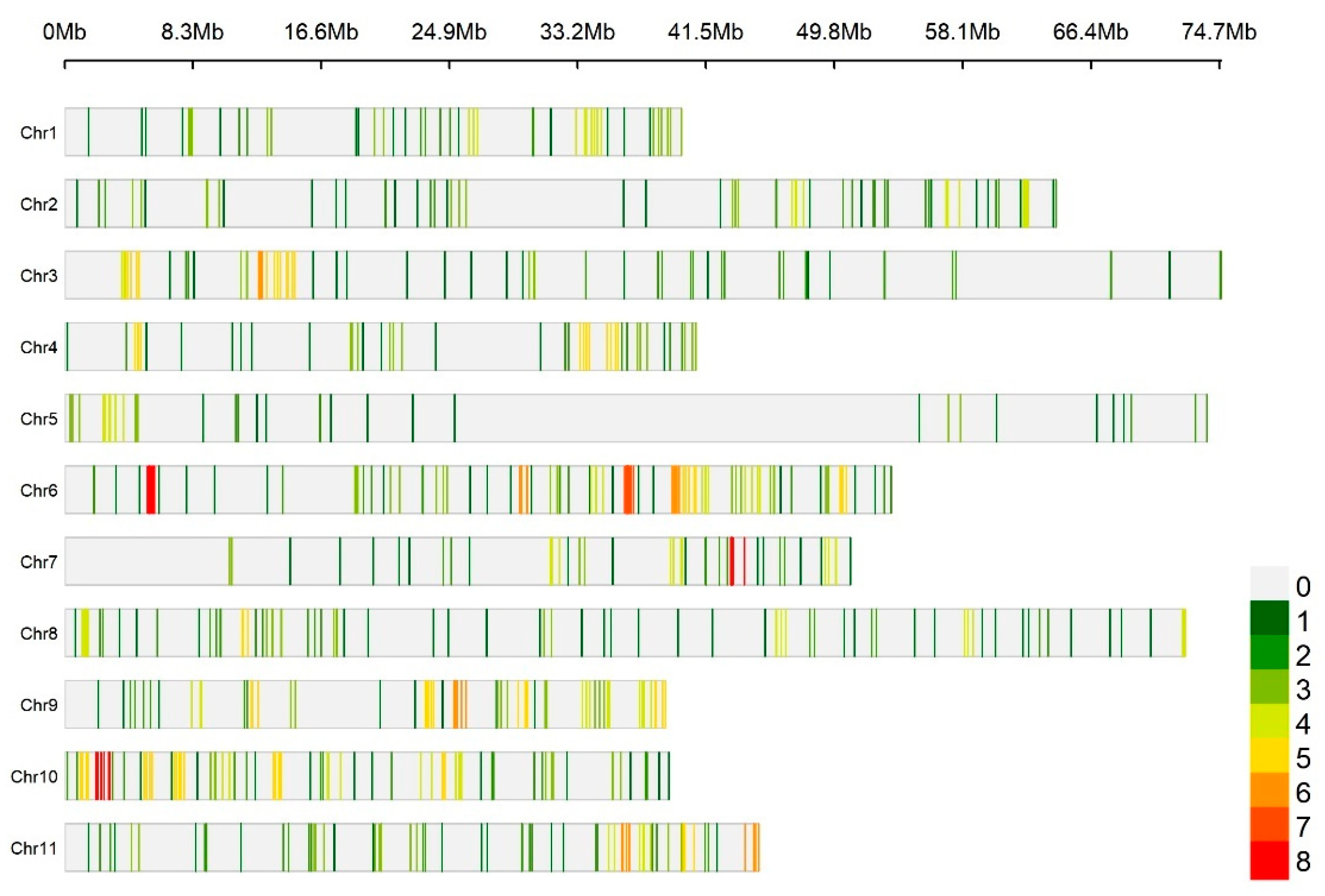
2.1. Kinship Analysis
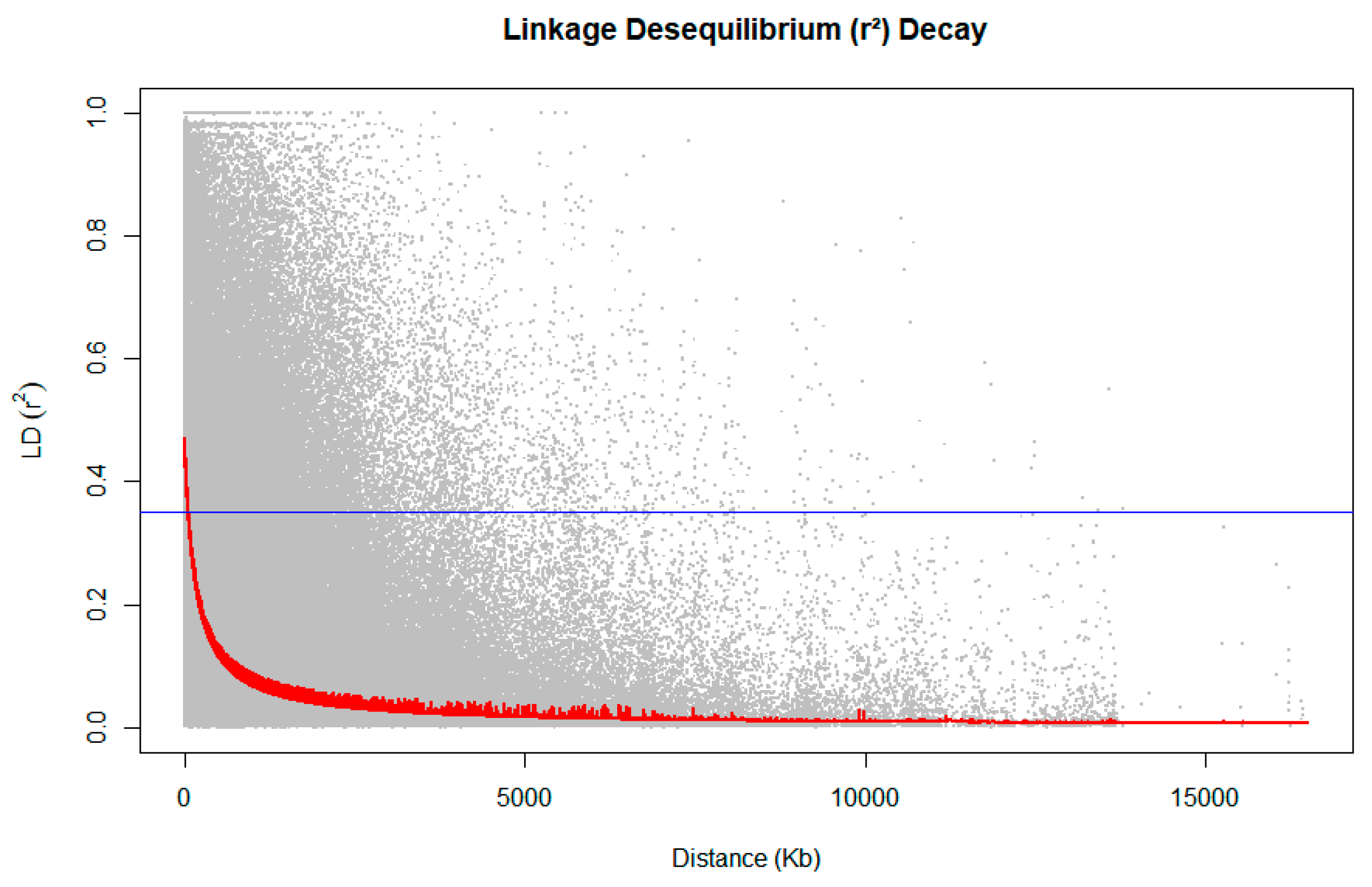
2.2. Decay of Linkage Disequilibrium
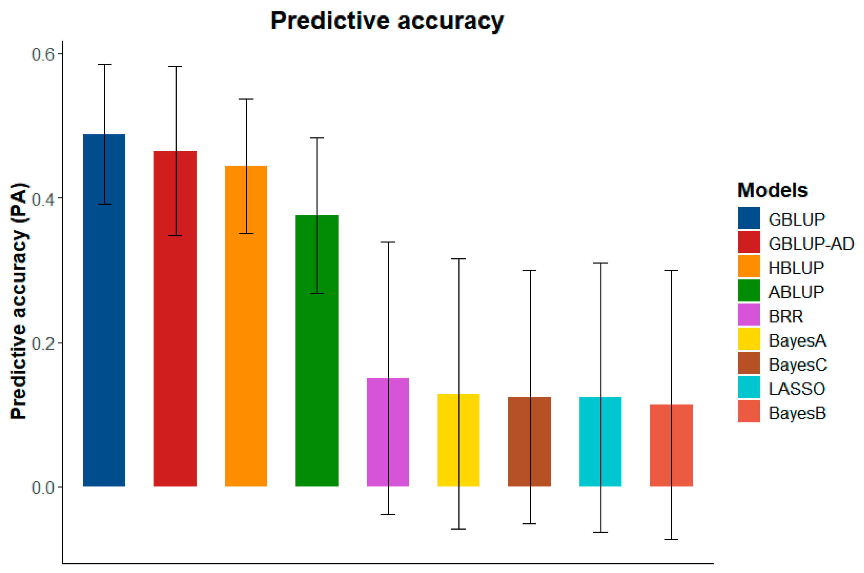
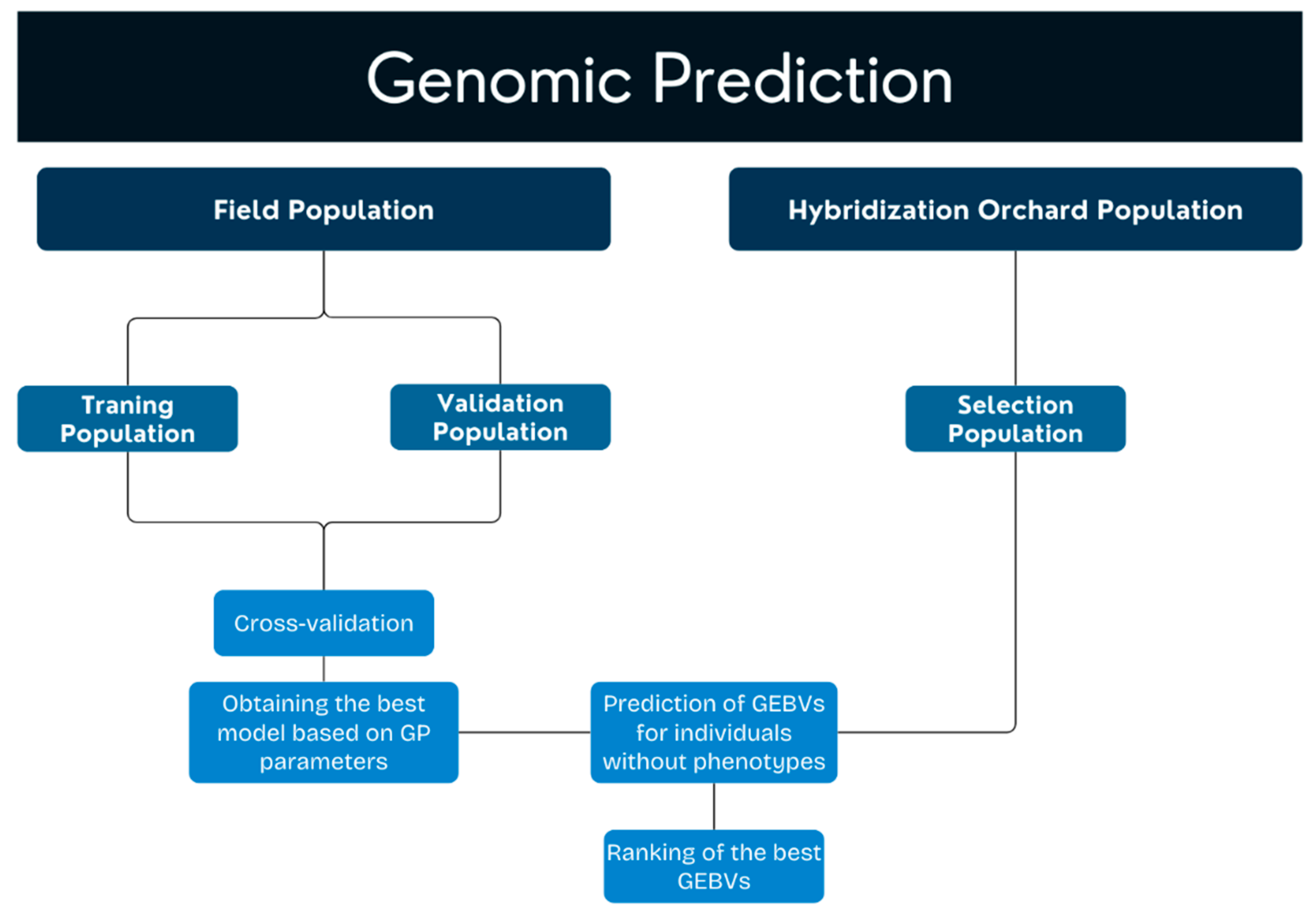
2.3. Genomic Selection
3. Discussion
3.1. Linkage Disequilibrium
3.2. Genomic Selection and Prediction
4. Conclusions
5. Material and Methods
5.1. Study Population
5.1.1. Obtaining Seeds and Paternity Testing
5.1.2. Individuals in the Field and in the Hybridization Orchard
5.2. Genotyping and Quality Control of SNPs
5.3. Linkage Disequilibrium (LD)
5.4. Genomic Selection
- 1.
- Predictive capacity (PC): the strength of the relationship between the predicted values and the actual observed values. It quantifies how well the model predicts the genotypes. A PC value closer to 1 indicates a better predictive accuracy of the model. The PC [69] formula iswhere is the covariance between the predicted values () and the actual values (), is the standard deviation of the variance of the predicted values, and is the standard deviation of the variance of the actual values.
- 2.
- Mean square error (MSE): the average squared difference between the predicted values and the actual values. It provides an understanding of how much error exists in the model’s predictions. The closer the MSE is to zero, the better the model is at predicting the values correctly. The MSE [70] formula iswhere are the predicted values, are the observed values, and n is the number of observations.
- 3.
- Coefficient of determination (): the proportion of variance in the observed data that is explained by the model. It indicates how well the model fits the data. An R2 value closer to 1 indicates that the model explains most of the variance in the data and thus is performing well. The formula for R2 [71] iswhere is the sum of squares of the residuals (the unexplained variance) and is the total sum of squares (the total variance in the data).
Author Contributions
Funding
Data Availability Statement
Acknowledgments
Conflicts of Interest
References
- Lebowitz, R.J.; Soller, M.; Beckmann, J.S. Trait-Based Analyses for the Detection of Linkage between Marker Loci and Quantitative Trait Loci in Crosses between Inbred Lines. Theor. Appl. Genet. 1987, 73, 556–562. [Google Scholar] [CrossRef] [PubMed]
- Hayes, B.J.; Chamberlain, A.J.; McPartlan, H.; Macleod, I.; Sethuraman, L.; Goddard, M.E. Accuracy of Marker-Assisted Selection with Single Markers and Marker Haplotypes in Cattle. Genet. Res. 2007, 89, 215–220. [Google Scholar] [CrossRef] [PubMed]
- Grattapaglia, D.; Kirst, M. Eucalyptus Applied Genomics: From Gene Sequences to Breeding Tools. New Phytol. 2008, 179, 911–929. [Google Scholar] [CrossRef] [PubMed]
- Meuwissen, T.H.E.; Hayes, B.J.; Goddard, M.E. Prediction of Total Genetic Value Using Genome-Wide Dense Marker Maps. Genetics 2001, 157, 1819–1829. [Google Scholar] [CrossRef]
- Denis, M.; Bouvet, J.-M. Efficiency of Genomic Selection with Models Including Dominance Effect in the Context of Eucalyptus Breeding. Tree Genet. Genomes 2013, 9, 37–51. [Google Scholar] [CrossRef]
- Rezende, B.A. Seleção Genômica Ampla para Volume e Qualidade da Madeira em Eucalipto. Ph.D. Thesis, Universidade Federal de Lavras, Lavras, Brazil, 2015. [Google Scholar]
- Resende, M.D.V.; Resende, M.F.R., Jr.; Sansaloni, C.P.; Petroli, C.D.; Missiaggia, A.A.; Aguiar, A.M.; Abad, J.M.; Takahashi, E.K.; Rosado, A.M.; Faria, D.A.; et al. Genomic Selection for Growth and Wood Quality in Eucalyptus: Capturing the Missing Heritability and Accelerating Breeding for Complex Traits in Forest Trees. New Phytol. 2012, 194, 116–128. [Google Scholar] [CrossRef]
- Heffner, E.L.; Sorrells, M.E.; Jannink, J.-L. Genomic Selection for Crop Improvement. Crop Sci. 2009, 49, 1–12. [Google Scholar] [CrossRef]
- Daetwyler, H.D.; Villanueva, B.; Woolliams, J.A. Accuracy of Predicting the Genetic Risk of Disease Using a Genome-Wide Approach. PLoS ONE 2008, 3, e3395. [Google Scholar] [CrossRef]
- Crossa, J.; Pérez-Rodríguez, P.; Cuevas, J.; Montesinos-López, O.; Jarquín, D.; De Los Campos, G.; Burgueño, J.; González-Camacho, J.M.; Pérez-Elizalde, S.; Beyene, Y.; et al. Genomic Selection in Plant Breeding: Methods, Models, and Perspectives. Trends Plant Sci. 2017, 22, 961–975. [Google Scholar] [CrossRef]
- Abdollahi-Arpanahi, R.; Morota, G.; Valente, B.d.; Kranis, A.; Rosa, G.j.m.; Gianola, D. Assessment of Bagging GBLUP for Whole-Genome Prediction of Broiler Chicken Traits. J. Anim. Breed. Genet. 2015, 132, 218–228. [Google Scholar] [CrossRef]
- Calus, M.P.; Huang, H.; Vereijken, A.; Visscher, J.; Ten Napel, J.; Windig, J.J. Genomic Prediction Based on Data from Three Layer Lines: A Comparison between Linear Methods. Genet. Sel. Evol. 2014, 46, 57. [Google Scholar] [CrossRef] [PubMed]
- Lopez-Cruz, M.; Crossa, J.; Bonnett, D.; Dreisigacker, S.; Poland, J.; Jannink, J.-L.; Singh, R.P.; Autrique, E.; de los Campos, G. Increased Prediction Accuracy in Wheat Breeding Trials Using a Marker × Environment Interaction Genomic Selection Model. G3 Genes Genomes Genet. 2015, 5, 569–582. [Google Scholar] [CrossRef] [PubMed]
- Hayes, B.J.; Bowman, P.J.; Chamberlain, A.J.; Goddard, M.E. Invited Review: Genomic Selection in Dairy Cattle: Progress and Challenges. J. Dairy Sci. 2009, 92, 433–443. [Google Scholar] [CrossRef] [PubMed]
- Benatti, T.R.; Ferreira, F.M.; da Costa, R.M.L.; de Moraes, M.L.T.; Aguiar, A.M.; da Costa Dias, D.; de Matos, J.W.; Fernandes, A.C.M.; Andrade, M.C.; de Siqueira, L.; et al. Accelerating Eucalypt Clone Selection Pipeline via Cloned Progeny Trials and Molecular Data. Plant Methods 2025, 21, 19. [Google Scholar] [CrossRef]
- Grattapaglia, D.; Silva-Junior, O.B.; Resende, R.T.; Cappa, E.P.; Müller, B.S.F.; Tan, B.; Isik, F.; Ratcliffe, B.; El-Kassaby, Y.A. Quantitative Genetics and Genomics Converge to Accelerate Forest Tree Breeding. Front. Plant Sci. 2018, 9, 1693. [Google Scholar] [CrossRef]
- Frisch, M.; Melchinger, A.E. Variance of the Parental Genome Contribution to Inbred Lines Derived From Biparental Crosses. Genetics 2007, 176, 477–488. [Google Scholar] [CrossRef]
- Hufford, M.B.; Xu, X.; van Heerwaarden, J.; Pyhäjärvi, T.; Chia, J.-M.; Cartwright, R.A.; Elshire, R.J.; Glaubitz, J.C.; Guill, K.E.; Kaeppler, S.M.; et al. Comparative Population Genomics of Maize Domestication and Improvement. Nat. Genet. 2012, 44, 808–811. [Google Scholar] [CrossRef]
- Sprague, G.F.; Tatum, L.A. General vs. Specific Combining Ability in Single Crosses of Corn. J. Am. Soc. Agron. 1942, 34, 923–932. [Google Scholar] [CrossRef]
- Duvick, D.N. The Contribution of Breeding to Yield Advances in Maize (Zea mays L.). Adv. Agron. 2005, 86, 83–145. [Google Scholar] [CrossRef]
- Allard, R.W. Principles of Plant Breeding; John Wiley & Sons: Hoboken, NJ, USA, 1999. [Google Scholar]
- Bernardo, R. Molecular Markers and Selection for Complex Traits in Plants: Learning from the Last 20 Years. Crop Sci. 2008, 48, 1649–1664. [Google Scholar] [CrossRef]
- Flint-Garcia, S.A.; Thornsberry, J.M.; Iv, E.S.B. Structure of Linkage Disequilibrium in Plants. Annu. Rev. Plant Biol. 2003, 54, 357–374. [Google Scholar] [CrossRef] [PubMed]
- Paes, G.P. Desequilíbrio de Ligação e Mapeamento Associativo em Populações de Milho-Pipoca Relacionadas por ciclos de Seleção. Master’s Thesis, Universidade Federal de Viçosa, Viçosa, Brazil, 2014. [Google Scholar]
- Hartl, D.L.; Clark, A.G.; Clark, A.G. Principles of Population Genetics; Sinauer Associates: Sunderland, MA, USA, 1997; Volume 116. [Google Scholar]
- Charlesworth, D.; Willis, J.H. The Genetics of Inbreeding Depression. Nat. Rev. Genet. 2009, 10, 783–796. [Google Scholar] [CrossRef] [PubMed]
- Estopa, R.A.; Paludeto, J.G.Z.; Müller, B.S.F.; de Oliveira, R.A.; Azevedo, C.F.; de Resende, M.D.V.; Tambarussi, E.V.; Grattapaglia, D. Genomic Prediction of Growth and Wood Quality Traits in Eucalyptus benthamii Using Different Genomic Models and Variable SNP Genotyping Density. New For. 2023, 54, 343–362. [Google Scholar] [CrossRef]
- Wientjes, Y.C.J.; Bijma, P.; Veerkamp, R.F.; Calus, M.P.L. An Equation to Predict the Accuracy of Genomic Values by Combining Data from Multiple Traits, Populations, or Environments. Genetics 2016, 202, 799–823. [Google Scholar] [CrossRef]
- Viana, J.M.S.; Garcia, A.A.F. Significance of Linkage Disequilibrium and Epistasis on Genetic Variances in Noninbred and Inbred Populations. BMC Genom. 2022, 23, 286. [Google Scholar] [CrossRef]
- Scutari, M.; Mackay, I.; Balding, D. Improving the Efficiency of Genomic Selection. Stat. Appl. Genet. Mol. Biol. 2013, 12, 517–527. [Google Scholar] [CrossRef]
- Tambarussi, E.V.; Shalizi, M.N.; Grattapaglia, D.; Hodge, G.; Isik, F.; Paludeto, J.G.Z.; Biernaski, F.A.; Acosta, J.J. Genome-Wide SNP-Based Relationships Improve Genetic Parameter Estimates and Genomic Prediction of Growth Traits in a Large Operational Breeding Trials of Pinus taeda L. For. Int. J. For. Res. 2025, cpaf004. [Google Scholar] [CrossRef]
- Shi, S.; Li, X.; Fang, L.; Liu, A.; Su, G.; Zhang, Y.; Luobu, B.; Ding, X.; Zhang, S. Genomic Prediction Using Bayesian Regression Models With Global–Local Prior. Front. Genet. 2021, 12, 628205. [Google Scholar] [CrossRef]
- Freitas, T.P.; Oliveira, J.T.D.S.; Paes, J.B.; Vidaurre, G.B.; Lima, J.L. Environmental Effect on Growth and Characteristics of Eucalyptus Wood. Floresta Ambient. 2019, 26, e20160302. [Google Scholar] [CrossRef]
- Takahashi, Y.; Ueki, M.; Tamiya, G.; Ogishima, S.; Kinoshita, K.; Hozawa, A.; Minegishi, N.; Nagami, F.; Fukumoto, K.; Otsuka, K.; et al. Machine Learning for Effectively Avoiding Overfitting Is a Crucial Strategy for the Genetic Prediction of Polygenic Psychiatric Phenotypes. Transl. Psychiatry 2020, 10, 1–11. [Google Scholar] [CrossRef]
- Montesinos-López, O.A.; Crespo-Herrera, L.; Xavier, A.; Godwa, M.; Beyene, Y.; Pierre, C.S.; de la Rosa-Santamaria, R.; Salinas-Ruiz, J.; Gerard, G.; Vitale, P.; et al. A Marker Weighting Approach for Enhancing Within-Family Accuracy in Genomic Prediction. G3 Genes Genomes Genet. 2024, 14, jkad278. [Google Scholar] [CrossRef] [PubMed]
- Windhausen, V.S.; Atlin, G.N.; Hickey, J.M.; Crossa, J.; Jannink, J.-L.; Sorrells, M.E.; Raman, B.; Cairns, J.E.; Tarekegne, A.; Semagn, K.; et al. Effectiveness of Genomic Prediction of Maize Hybrid Performance in Different Breeding Populations and Environments. G3 Genes Genomes Genet. 2012, 2, 1427–1436. [Google Scholar] [CrossRef] [PubMed]
- Peixoto, M.A.; Leach, K.A.; Jarquin, D.; Flannery, P.; Zystro, J.; Tracy, W.F.; Bhering, L.; Resende, M.F.R. Utilizing Genomic Prediction to Boost Hybrid Performance in a Sweet Corn Breeding Program. Front. Plant Sci. 2024, 15, 1293307. [Google Scholar] [CrossRef] [PubMed]
- Duarte, D.; Jurcic, E.J.; Dutour, J.; Villalba, P.V.; Centurión, C.; Grattapaglia, D.; Cappa, E.P. Genomic Selection in Forest Trees Comes to Life: Unraveling Its Potential in an Advanced Four-Generation Eucalyptus grandis Population. Front. Plant Sci. 2024, 15, 1462285. [Google Scholar] [CrossRef]
- Mphahlele, M.M.; Isik, F.; Mostert-O’Neill, M.M.; Reynolds, S.M.; Hodge, G.R.; Myburg, A.A. Expected Benefits of Genomic Selection for Growth and Wood Quality Traits in Eucalyptus grandis. Tree Genet. Genomes 2020, 16, 49. [Google Scholar] [CrossRef]
- Grattapaglia, D.; Vilela Resende, M.D.; Resende, M.R.; Sansaloni, C.P.; Petroli, C.D.; Missiaggia, A.A.; Takahashi, E.K.; Zamprogno, K.C.; Kilian, A. Genomic Selection for Growth Traits in Eucalyptus: Accuracy within and across Breeding Populations. BMC Proc 2011, 5, O16. [Google Scholar] [CrossRef]
- Schafer, J.L.; Graham, J.W. Missing Data: Our View of the State of the Art. Psychol. Methods 2002, 7, 147–177. [Google Scholar] [CrossRef]
- Robert, P.; Auzanneau, J.; Goudemand, E.; Oury, F.-X.; Rolland, B.; Heumez, E.; Bouchet, S.; Le Gouis, J.; Rincent, R. Phenomic Selection in Wheat Breeding: Identification and Optimisation of Factors Influencing Prediction Accuracy and Comparison to Genomic Selection. Theor. Appl. Genet. 2022, 135, 895–914. [Google Scholar] [CrossRef]
- Ceballos, F.C.; Joshi, P.K.; Clark, D.W.; Ramsay, M.; Wilson, J.F. Runs of Homozygosity: Windows into Population History and Trait Architecture. Nat. Rev. Genet. 2018, 19, 220–234. [Google Scholar] [CrossRef]
- Ornella, L.; Singh, S.; Perez, P.; Burgueño, J.; Singh, R.; Tapia, E.; Bhavani, S.; Dreisigacker, S.; Braun, H.-J.; Mathews, K.; et al. Genomic Prediction of Genetic Values for Resistance to Wheat Rusts. Plant Genome 2012, 5, 136–148. [Google Scholar] [CrossRef]
- Heidaritabar, M.; Wolc, A.; Arango, J.; Zeng, J.; Settar, P.; Fulton, J.e.; O’Sullivan, N.P.; Bastiaansen, J.W.M.; Fernando, R.L.; Garrick, D.J.; et al. Impact of Fitting Dominance and Additive Effects on Accuracy of Genomic Prediction of Breeding Values in Layers. J. Anim. Breed. Genet. 2016, 133, 334–346. [Google Scholar] [CrossRef] [PubMed]
- Liang, Z.; Gupta, S.K.; Yeh, C.-T.; Zhang, Y.; Ngu, D.W.; Kumar, R.; Patil, H.T.; Mungra, K.D.; Yadav, D.V.; Rathore, A.; et al. Phenotypic Data from Inbred Parents Can Improve Genomic Prediction in Pearl Millet Hybrids. G3 Genes Genomes Genet. 2018, 8, 2513–2522. [Google Scholar] [CrossRef] [PubMed]
- Wright, S.I.; Ness, R.W.; Foxe, J.P.; Barrett, S.C.H. Genomic Consequences of Outcrossing and Selfing in Plants. Int. J. Plant Sci. 2008, 169, 105–118. [Google Scholar] [CrossRef]
- Weber, S.E.; Frisch, M.; Snowdon, R.J.; Voss-Fels, K.P. Haplotype Blocks for Genomic Prediction: A Comparative Evaluation in Multiple Crop Datasets. Front. Plant Sci. 2023, 14, 1217589. [Google Scholar] [CrossRef]
- Fernando, R.L.; Cheng, H.; Garrick, D.J. An Efficient Exact Method to Obtain GBLUP and Single-Step GBLUP When the Genomic Relationship Matrix Is Singular. Genet. Sel. Evol. 2016, 48, 80. [Google Scholar] [CrossRef]
- Valente, S.; Ribeiro, M.; Schnur, J.; Alves, F.; Moniz, N.; Seelow, D.; Freixo, J.P.; Silva, P.F.; Oliveira, J. Analysis of Regions of Homozygosity: Revisited Through New Bioinformatic Approaches. BioMedInformatics 2024, 4, 2374–2399. [Google Scholar] [CrossRef]
- Li, W.; Zhang, M.; Du, H.; Wu, J.; Zhou, L.; Liu, J. Multi-Trait Bayesian Models Enhance the Accuracy of Genomic Prediction in Multi-Breed Reference Populations. Agriculture 2024, 14, 626. [Google Scholar] [CrossRef]
- Isik, F. Genomic Selection in Forest Tree Breeding: The Concept and an Outlook to the Future. New For. 2014, 45, 379–401. [Google Scholar] [CrossRef]
- Jhariya, M.; Raj, D.; Sahu, P.; Singh, N.R.; Sahu, K. Molecular Marker -a New Approach for Forest Tree Improvement. Ecol. Environ. Conserv. 2014, 20, 1101–1107. [Google Scholar]
- Cappa, E.P.; De Lima, B.M.; Da Silva-Junior, O.B.; Garcia, C.C.; Mansfield, S.D.; Grattapaglia, D. Improving Genomic Prediction of Growth and Wood Traits in Eucalyptus Using Phenotypes from Non-Genotyped Trees by Single-Step GBLUP. Plant Sci. 2019, 284, 9–15. [Google Scholar] [CrossRef]
- Marshall, T.C.; Slate, J.; Kruuk, L.E.B.; Pemberton, J.M. Statistical Confidence for Likelihood-based Paternity Inference in Natural Populations. Mol. Ecol. 1998, 7, 639–655. [Google Scholar] [CrossRef] [PubMed]
- Silva-Junior, O.B.; Faria, D.A.; Grattapaglia, D. A Flexible Multi-species Genome-wide 60K SNP Chip Developed from Pooled Resequencing of 240 Eucalyptus Tree Genomes across 12 Species. New Phytol. 2015, 206, 1527–1540. [Google Scholar] [CrossRef] [PubMed]
- Mueller, J.C. Linkage Disequilibrium for Different Scales and Applications. Brief. Bioinform. 2004, 5, 355–364. [Google Scholar] [CrossRef]
- Bradbury, P.J.; Zhang, Z.; Kroon, D.E.; Casstevens, T.M.; Ramdoss, Y.; Buckler, E.S. TASSEL: Software for Association Mapping of Complex Traits in Diverse Samples. Bioinformatics 2007, 23, 2633–2635. [Google Scholar] [CrossRef] [PubMed]
- R Core Team. R: A Language and Environment for Statistical Computing; R Foundation for Statistical Computing: Vienna, Austria, 2023. [Google Scholar]
- Bhat, J.A.; Ali, S.; Salgotra, R.K.; Mir, Z.A.; Dutta, S.; Jadon, V.; Tyagi, A.; Mushtaq, M.; Jain, N.; Singh, P.K.; et al. Genomic Selection in the Era of Next Generation Sequencing for Complex Traits in Plant Breeding. Front. Genet. 2016, 7, 221. [Google Scholar] [CrossRef]
- Henderson, C.R. Applications of Linear Models in Animal Breeding; University of Guelph: Guelph, ON, Canada, 1984; Volume 462. [Google Scholar]
- VanRaden, P.M. Efficient Methods to Compute Genomic Predictions. J. Dairy Sci. 2008, 91, 4414–4423. [Google Scholar] [CrossRef]
- Vitezica, Z.G.; Varona, L.; Legarra, A. On the Additive and Dominant Variance and Covariance of Individuals Within the Genomic Selection Scope. Genetics 2013, 195, 1223–1230. [Google Scholar] [CrossRef]
- Legarra, A.; Aguilar, I.; Misztal, I. A Relationship Matrix Including Full Pedigree and Genomic Information. J. Dairy Sci. 2009, 92, 4656–4663. [Google Scholar] [CrossRef]
- Gianola, D.; de los Campos, G.; Hill, W.G.; Manfredi, E.; Fernando, R. Additive Genetic Variability and the Bayesian Alphabet. Genetics 2009, 183, 347–363. [Google Scholar] [CrossRef]
- Habier, D.; Fernando, R.L.; Dekkers, J.C.M. The Impact of Genetic Relationship Information on Genome-Assisted Breeding Values. Genetics 2007, 177, 2389–2397. [Google Scholar] [CrossRef]
- Park, T.; Casella, G. The Bayesian Lasso. J. Am. Stat. Assoc. 2008, 103, 681–686. [Google Scholar] [CrossRef]
- Berrar, D. Cross-Validation. In Encyclopedia of Bioinformatics and Computational Biology; Academic Press: Oxford, UK, 2018; Volume 1, pp. 542–545. [Google Scholar]
- Pearson, K.; Henrici, O.M.F.E. VII. Mathematical Contributions to the Theory of Evolution.—III. Regression, Heredity, and Panmixia. Philos. Trans. R. Soc. Lond. Ser. A Contain. Pap. Math. Phys. Character 1896, 187, 253–318. [Google Scholar] [CrossRef]
- Kuhn, M.; Johnson, K. Applied Predictive Modeling; Springer: New York, NY, USA, 2013; ISBN 978-1-4614-6848-6. [Google Scholar]
- Montgomery, D.C.; Runger, G.C. Applied Statistics and Probability for Engineers; John Wiley & Sons: Hoboken, NJ, USA, 2010; ISBN 978-0-470-05304-1. [Google Scholar]

| Parameters | ||
|---|---|---|
| Models | EQM | R2 |
| GBLUP | 13.336 (±1.930) | 0.225 (±0.105) |
| GBLUP-AD | 13.992 (±2.565) | 0.187 (±0.145) |
| HBLUP | 14.390 (±1.408) | 0.185 (±0.077) |
| ABLUP | 15.498 (±1.986) | 0.124 (±0.095) |
| BayesA | 3.721 (±0.222) | 0.048 (±0.053) |
| BayesB | 3.735 (±0.219) | 0.044 (±0.053) |
| BayesC | 3.732 (±0.231) | 0.043 (±0.043) |
| LASSO | 3.719 (±0.220) | 0.046 (±0.055) |
| BRR | 3.723 (±0.257) | 0.055 (±0.054) |
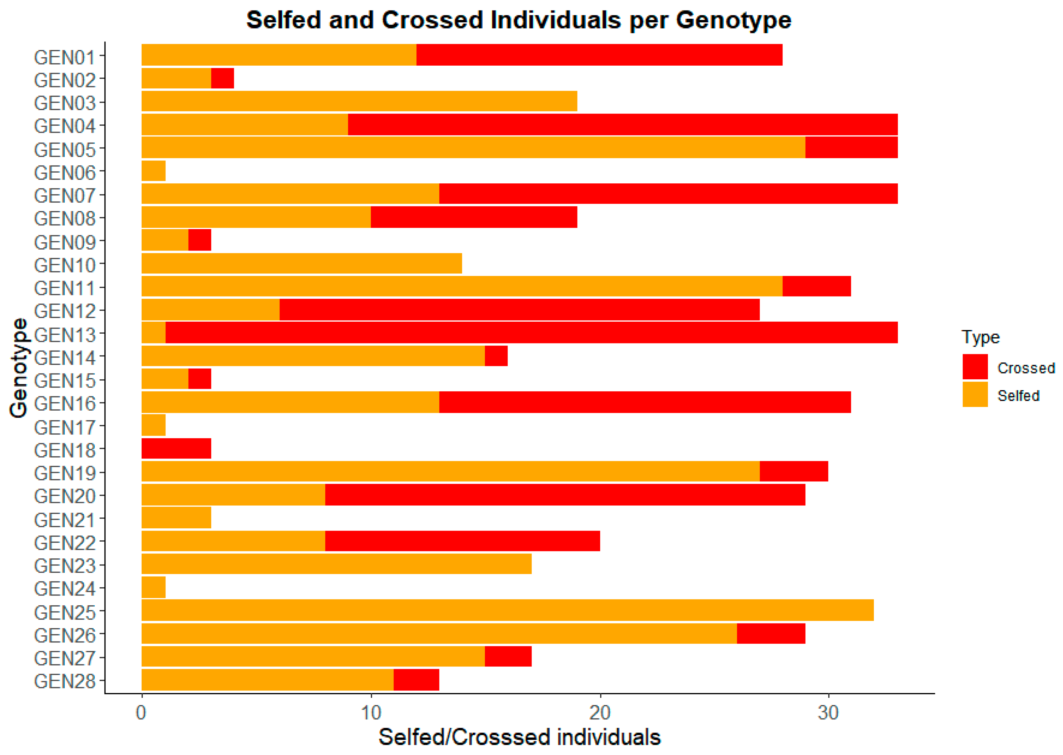
| Genotype | Ancestry | #Total Seeds | #Selfed | #Crossed | ||
|---|---|---|---|---|---|---|
| E. urophylla | E. grandis | Unknown | ||||
| GEN1 | 0.500 | 0.500 | 0.000 | 28 | 12 | 16 |
| GEN2 | 0.500 | 0.500 | 0.000 | 4 | 3 | 1 |
| GEN3 | 0.500 | 0.492 | 0.008 | 19 | 19 | 0 |
| GEN4 | 0.476 | 0.448 | 0.076 | 33 | 9 | 24 |
| GEN5 | 0.487 | 0.498 | 0.015 | 33 | 29 | 4 |
| GEN6 | 0.080 | 0.912 | 0.007 | 1 | 1 | 0 |
| GEN7 | 0.495 | 0.500 | 0.005 | 33 | 13 | 20 |
| GEN8 | 0.499 | 0.496 | 0.005 | 19 | 10 | 9 |
| GEN9 | 0.380 | 0.609 | 0.011 | 3 | 2 | 1 |
| GEN10 | 0.496 | 0.500 | 0.004 | 14 | 14 | 0 |
| GEN11 | 0.500 | 0.495 | 0.004 | 31 | 28 | 3 |
| GEN12 | 0.475 | 0.474 | 0.050 | 27 | 6 | 21 |
| GEN13 | 0.455 | 0.455 | 0.090 | 33 | 1 | 32 |
| GEN14 | 0.493 | 0.492 | 0.015 | 16 | 15 | 1 |
| GEN15 | 0.510 | 0.475 | 0.015 | 3 | 2 | 1 |
| GEN16 | 0.506 | 0.487 | 0.006 | 31 | 13 | 18 |
| GEN17 | 0.498 | 0.496 | 0.006 | 1 | 1 | 0 |
| GEN18 | 0.596 | 0.351 | 0.053 | 3 | 0 | 3 |
| GEN19 | 0.600 | 0.303 | 0.096 | 30 | 27 | 3 |
| GEN20 | 0.247 | 0.246 | 0.507 | 29 | 8 | 21 |
| GEN21 | 0.494 | 0.500 | 0.006 | 3 | 3 | 0 |
| GEN22 | 0.478 | 0.503 | 0.019 | 20 | 8 | 12 |
| GEN23 | 0.498 | 0.496 | 0.006 | 17 | 17 | 0 |
| GEN24 | 0.047 | 0.443 | 0.511 | 1 | 1 | 0 |
| GEN25 | 0.502 | 0.496 | 0.001 | 32 | 32 | 0 |
| GEN26 | 0.405 | 0.583 | 0.012 | 29 | 26 | 3 |
| GEN27 | 0.463 | 0.535 | 0.002 | 17 | 15 | 2 |
| GEN28 | 0.504 | 0.496 | 0.000 | 13 | 11 | 2 |
| Type | Model | Prior/Distribution |
|---|---|---|
| Frequentist | ABLUP | Additive Gaussian effects |
| GBLUP | Additive Gaussian effects | |
| GBLUP-AD | Additive and dominance Gaussian effects | |
| HBLUP | Combination of priors from A and G | |
| Bayesian | BRR | Gaussian prior for all markers |
| BayesA | t-distribution (or scaled-t) for marker effects | |
| BayesB | Mixture: probability p of zero effect and (1-p) t or normal | |
| BayesC | Mixture: probability p of zero effect and (1-p) normal | |
| Bayes Lasso | Laplace (L1) prior |
Disclaimer/Publisher’s Note: The statements, opinions and data contained in all publications are solely those of the individual author(s) and contributor(s) and not of MDPI and/or the editor(s). MDPI and/or the editor(s) disclaim responsibility for any injury to people or property resulting from any ideas, methods, instructions or products referred to in the content. |
© 2025 by the authors. Licensee MDPI, Basel, Switzerland. This article is an open access article distributed under the terms and conditions of the Creative Commons Attribution (CC BY) license (https://creativecommons.org/licenses/by/4.0/).
Share and Cite
Melchert, G.F.; Ferreira, F.M.; Muniz, F.R.; de Matos, J.W.; Benatti, T.R.; Brum, I.J.B.; de Siqueira, L.; Tambarussi, E.V. Genomic Prediction in a Self-Fertilized Progenies of Eucalyptus spp. Plants 2025, 14, 1422. https://doi.org/10.3390/plants14101422
Melchert GF, Ferreira FM, Muniz FR, de Matos JW, Benatti TR, Brum IJB, de Siqueira L, Tambarussi EV. Genomic Prediction in a Self-Fertilized Progenies of Eucalyptus spp. Plants. 2025; 14(10):1422. https://doi.org/10.3390/plants14101422
Chicago/Turabian StyleMelchert, Guilherme Ferreira, Filipe Manoel Ferreira, Fabiana Rezende Muniz, Jose Wilacildo de Matos, Thiago Romanos Benatti, Itaraju Junior Baracuhy Brum, Leandro de Siqueira, and Evandro Vagner Tambarussi. 2025. "Genomic Prediction in a Self-Fertilized Progenies of Eucalyptus spp." Plants 14, no. 10: 1422. https://doi.org/10.3390/plants14101422
APA StyleMelchert, G. F., Ferreira, F. M., Muniz, F. R., de Matos, J. W., Benatti, T. R., Brum, I. J. B., de Siqueira, L., & Tambarussi, E. V. (2025). Genomic Prediction in a Self-Fertilized Progenies of Eucalyptus spp. Plants, 14(10), 1422. https://doi.org/10.3390/plants14101422