
Medicinal Chrysanthemum Detection under Complex Environments Using the MC-LCNN Model

Abstract
:1. Introduction
- A lightweight MC-LCNN model was designed to achieve high-accuracy, real-time detection of medicinal chrysanthemums under complex unstructured environments.
- A series of experiments were designed to validate the superiority of MC-LCNN, including comparisons with different data enhancements, ablation experiments between various network components, and comparisons with state-of-the-art object detection models.
- The MC-LCNN model was embedded into an edge computing device with a custom pipeline design to achieve accurate real-time medicinal chrysanthemum detection.
2. Materials and Methods
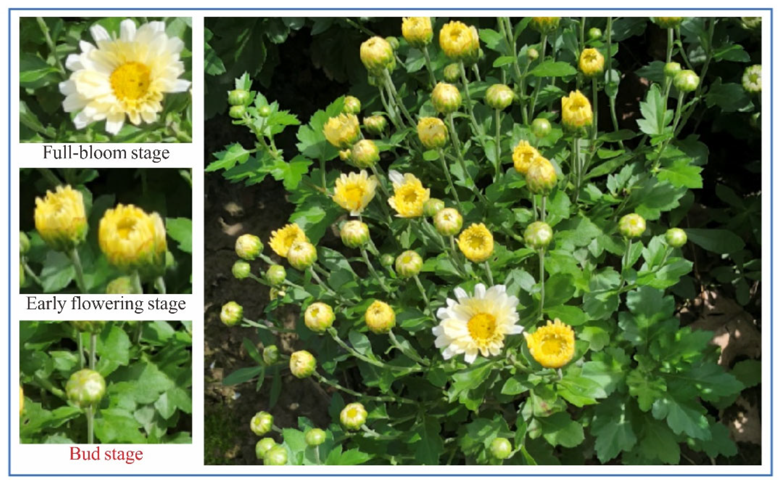
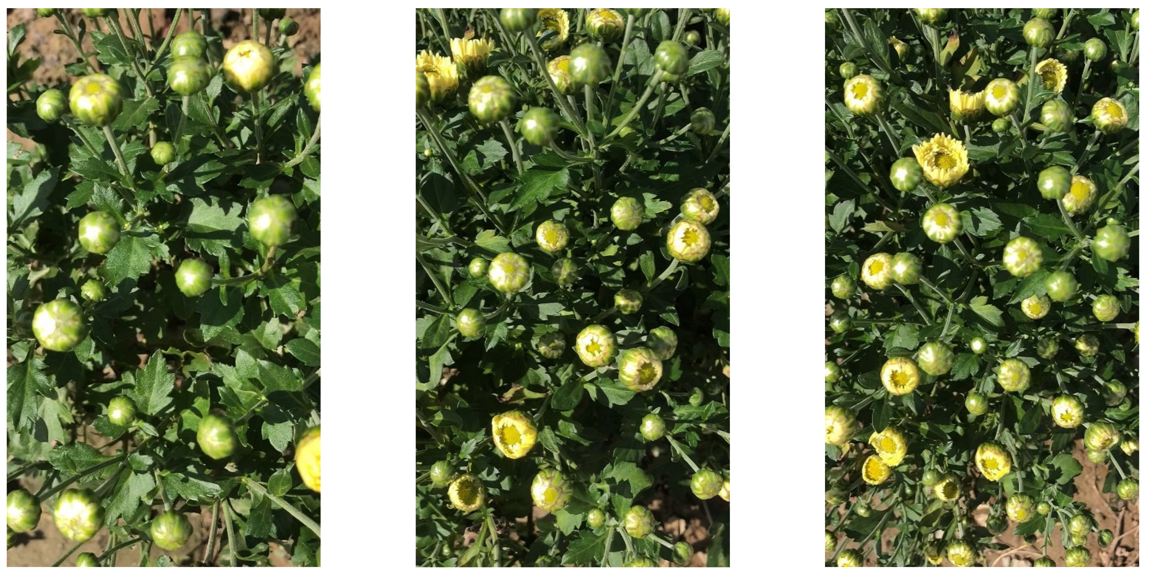
2.1. Dataset
2.2. NVIDIA Jetson TX2
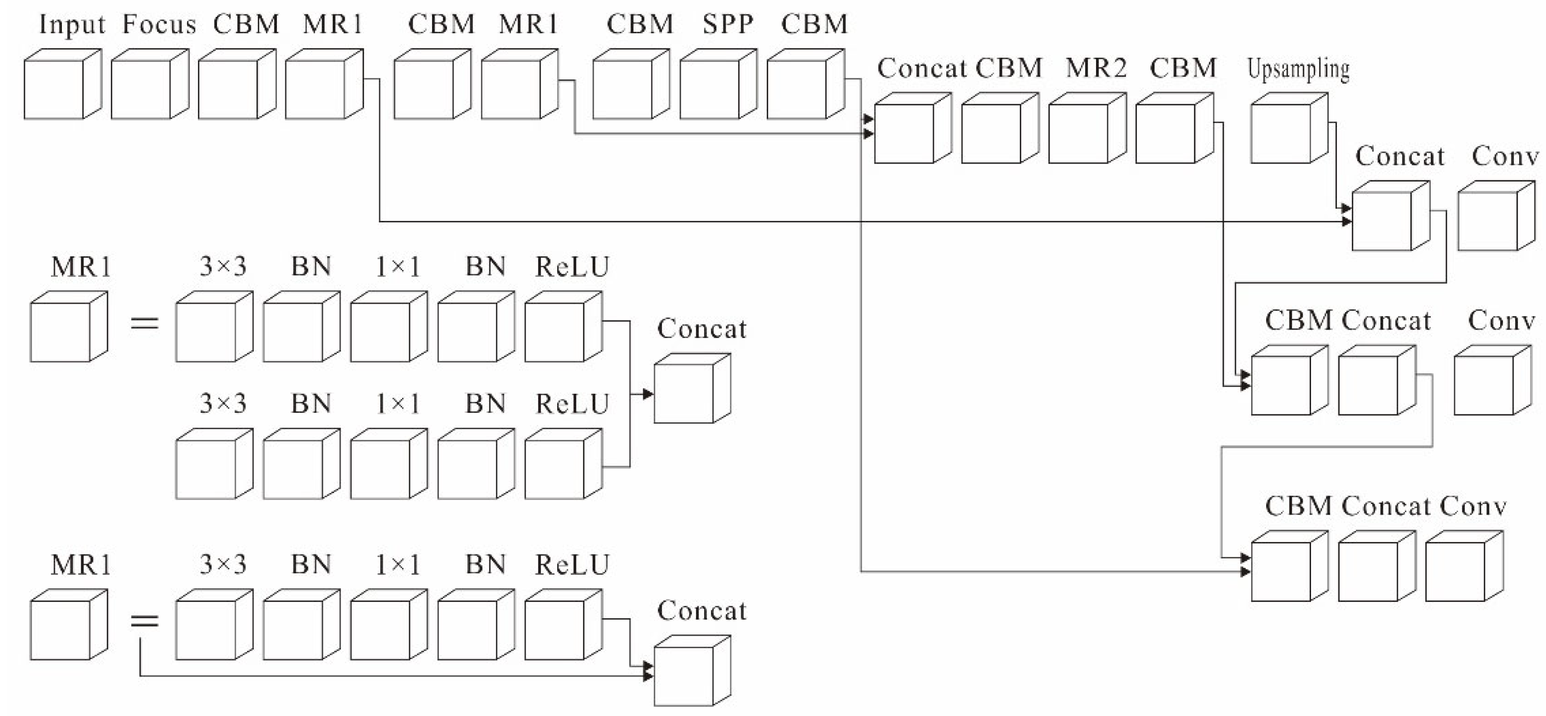
2.3. MC-LCNN
2.3.1. MC-ResNetv1 and MC-ResNetv2
2.3.2. Generalized Focal Loss
2.4. CPU–GPU Multithreaded Pipeline Design
2.5. Evaluation Metrics
Experimental Setup
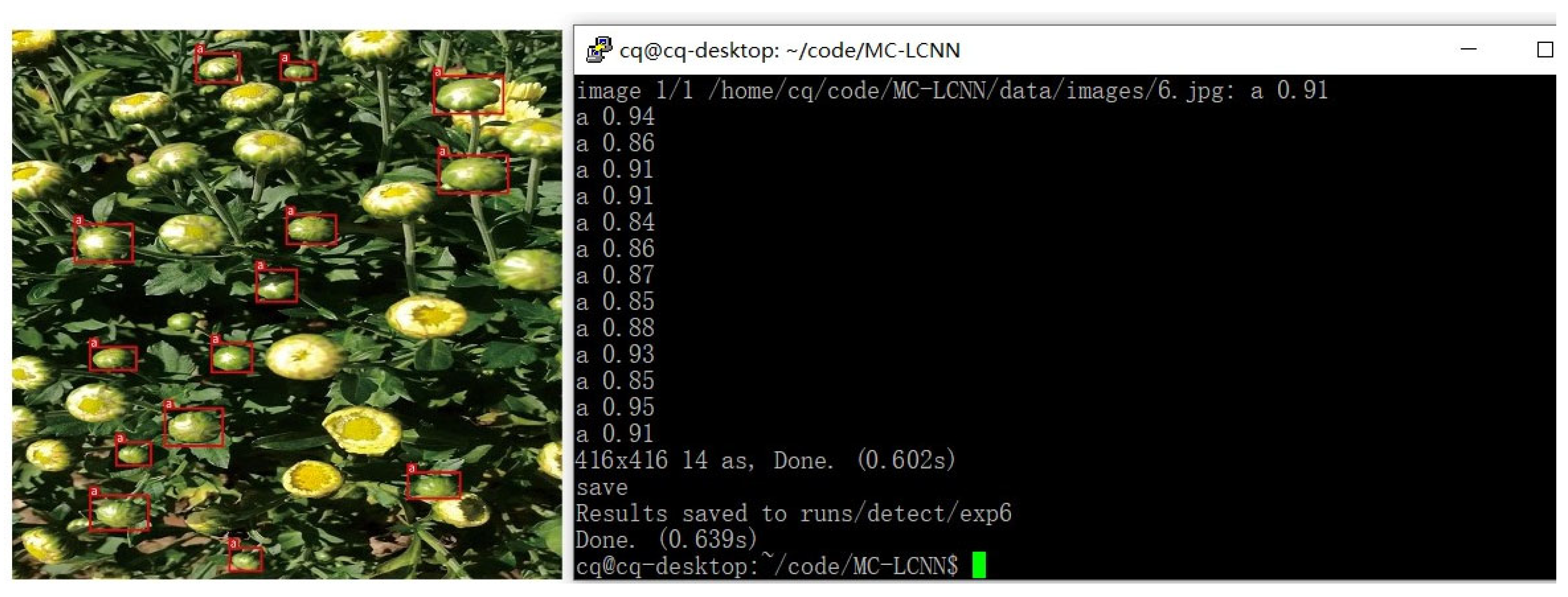
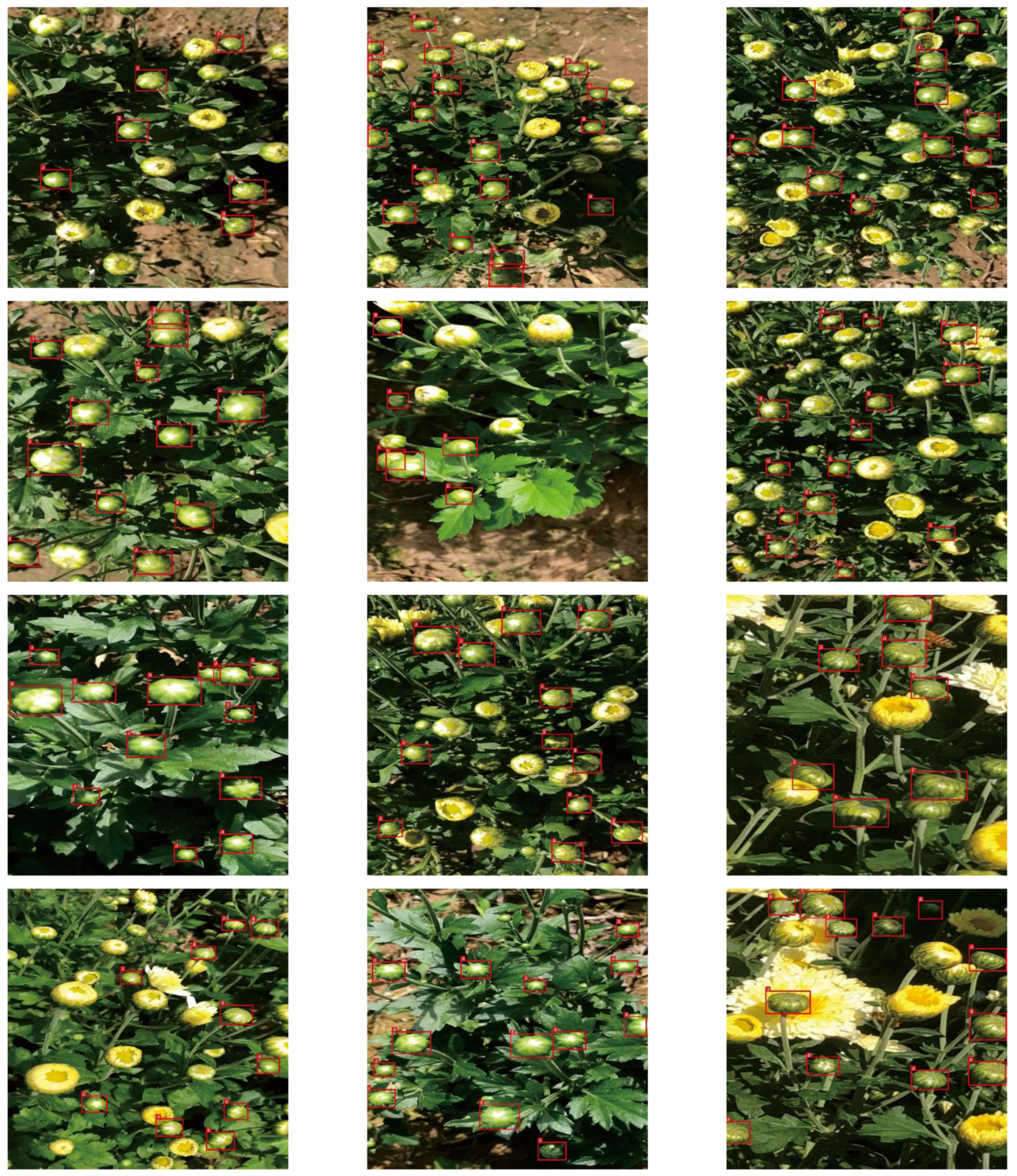
3. Results
3.1. The Impact of Data Augmentation on the MC-LCNN
3.2. Ablation Experiments
3.3. Comparisons with State-of-the-Art Detection Methods
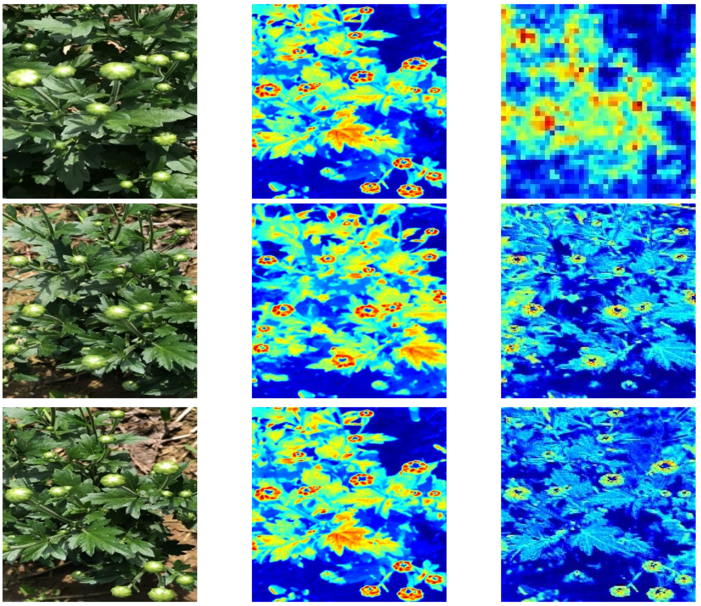
4. Discussion
5. Conclusions
Author Contributions
Funding
Institutional Review Board Statement
Informed Consent Statement
Data Availability Statement
Acknowledgments
Conflicts of Interest
References
- Liu, C.L.; Lu, W.Y.; Gao, B.Y.; Kimura, H.; Li, Y.F.; Wang, J. Rapid identification of chrysanthemum teas by computer vision and deep learning. Food Sci. Nutr. 2020, 8, 1968–1977. [Google Scholar] [CrossRef] [PubMed] [Green Version]
- Yuan, H.; Jiang, S.; Liu, Y.; Daniyal, M.; Jian, Y.; Peng, C.; Shen, J.; Liu, S.; Wang, W. The flower head of Chrysanthemum morifolium Ramat. (Juhua): A paradigm of flowers serving as Chinese dietary herbal medicine. J. Ethnopharmacol. 2020, 261, 113043. [Google Scholar] [CrossRef] [PubMed]
- Hasan, R.I.; Yusuf, S.M.; Alzubaidi, L. Review of the State of the Art of Deep Learning for Plant Diseases: A Broad Analysis and Discussion. Plants 2020, 9, 1302. [Google Scholar] [CrossRef] [PubMed]
- Wöber, W.; Mehnen, L.; Sykacek, P.; Meimberg, H. Investigating Explanatory Factors of Machine Learning Models for Plant Classification. Plants 2021, 10, 2674. [Google Scholar] [CrossRef] [PubMed]
- Genaev, M.A.; Skolotneva, E.S.; Gultyaeva, E.I.; Orlova, E.A.; Bechtold, N.P.; Afonnikov, D.A. Image-Based Wheat Fungi Diseases Identification by Deep Learning. Plants 2021, 10, 1500. [Google Scholar] [CrossRef] [PubMed]
- Kondo, N.; Ogawa, Y.; Monta, M.; Shibano, Y. Visual Sensing Algorithm For Chrysanthemum Cutting Sticking Robot System. In Proceedings of the International Society for Horticultural Science (ISHS), Leuven, Belgium, 1 December 1996; pp. 383–388. [Google Scholar]
- Warren, D. Image analysis in chrysanthemum DUS testing. Comput. Electron. Agric. 2000, 25, 213–220. [Google Scholar] [CrossRef]
- Tarry, C.; Wspanialy, P.; Veres, M.; Moussa, M. An Integrated Bud Detection and Localization System for Application in Greenhouse Automation. In Proceedings of the Canadian Conference on Computer and Robot Vision, Montreal, QC, Canada, 6–9 May 2014; pp. 344–348. [Google Scholar]
- Tete, T.N.; Kamlu, S. Detection of plant disease using threshold, k-mean cluster and ann algorithm. In Proceedings of the 2nd International Conference for Convergence in Technology (I2CT), Mumbai, India, 7–9 April 2017; pp. 523–526. [Google Scholar]
- Yang, Q.H.; Chang, C.; Bao, G.J.; Fan, J.; Xun, Y. Recognition and localization system of the robot for harvesting Hangzhou White Chrysanthemums. Int. J. Agric. Biol. Eng. 2018, 11, 88–95. [Google Scholar] [CrossRef]
- Yang, Q.H.; Luo, S.L.; Chang, C.; Xun, Y.; Bao, G.J. Segmentation algorithm for Hangzhou white chrysanthemums based on least squares support vector machine. Int. J. Agric. Biol. Eng. 2019, 12, 127–134. [Google Scholar] [CrossRef]
- Liu, Z.L.; Wang, J.; Tian, Y.; Dai, S.L. Deep learning for image-based large-flowered chrysanthemum cultivar recognition. Plant Methods 2019, 15, 146. [Google Scholar] [CrossRef] [PubMed]
- Van Nam, N. Application of the Faster R-CNN algorithm to identify objects with both noisy and noiseless images. Int. J. Adv. Res. Comput. Eng. Technol. 2020, 9, 112–115. [Google Scholar]
- Lin, T.; Goyal, P.; Girshick, R.; He, K.; Dollár, P. Focal Loss for Dense Object Detection. IEEE Trans. Pattern Anal. Mach. Intell. 2020, 42, 318–327. [Google Scholar] [CrossRef] [PubMed] [Green Version]
- Tian, Y.N.; Yang, G.D.; Wang, Z.; Li, E.; Liang, Z.Z. Instance segmentation of apple flowers using the improved mask R-CNN model. Biosyst. Eng. 2020, 193, 264–278. [Google Scholar] [CrossRef]
- Espejo-Garcia, B.; Mylonas, N.; Athanasakos, L.; Vali, E.; Fountas, S. Combining generative adversarial networks and agricultural transfer learning for weeds identification. Biosyst. Eng. 2021, 204, 79–89. [Google Scholar] [CrossRef]
- Ma, R.; Tao, P.; Tang, H.Y. Optimizing Data Augmentation for Semantic Segmentation on Small-Scale Dataset. In Proceedings of the 2nd International Conference on Control and Computer Vision (ICCCV), New York, NY, USA, 6–9 June 2019; pp. 77–81. [Google Scholar]
- Pandian, J.A.; Geetharamani, G.; Annette, B. Data Augmentation on Plant Leaf Disease Image Dataset Using Image Manipulation and Deep Learning Techniques. In Proceedings of the IEEE 9th International Conference on Advanced Computing (IACC), Tamilnadu, India, 13–14 December 2019; pp. 199–204. [Google Scholar]
- Dou, Z.; Gao, K.; Zhang, X.; Wang, H.; Wang, J. Improving Performance and Adaptivity of Anchor-Based Detector Using Differentiable Anchoring With Efficient Target Generation. IEEE Trans. Image Process. 2021, 30, 712–724. [Google Scholar] [CrossRef] [PubMed]
- Wu, D.H.; Lv, S.C.; Jiang, M.; Song, H.B. Using channel pruning-based YOLO v4 deep learning algorithm for the real-time and accurate detection of apple flowers in natural environments. Comput. Electron. Agric. 2020, 178, 12. [Google Scholar] [CrossRef]
- Zhang, T.; Li, L. An Improved Object Detection Algorithm Based on M2Det. In Proceedings of the IEEE International Conference on Artificial Intelligence and Computer Applications (ICAICA), Dalian, China, 27–29 June 2020; pp. 582–585. [Google Scholar]
- Hsu, W.Y.; Lin, W.Y. Ratio-and-Scale-Aware YOLO for Pedestrian Detection. IEEE Trans. Image Process. 2021, 30, 934–947. [Google Scholar] [CrossRef] [PubMed]
- Kim, S.W.; Kook, H.K.; Sun, J.Y.; Kang, M.C.; Ko, S.J. Parallel Feature Pyramid Network for Object Detection. In Proceedings of the European Conference on Computer Vision (ECCV), Munich, Germany, 8–14 September 2018; pp. 234–250. [Google Scholar]
- Wang, Z.; Cheng, Z.; Huang, H.; Zhao, J. ShuDA-RFBNet for Real-time Multi-task Traffic Scene Perception. In Proceedings of the Chinese Automation Congress (CAC), Hangzhou, China, 22–24 November 2019; pp. 305–310. [Google Scholar]
- Zhang, S.; Wen, L.; Lei, Z.; Li, S.Z. RefineDet++: Single-Shot Refinement Neural Network for Object Detection. IEEE Trans Circuits Syst. Video Technol. 2021, 31, 674–687. [Google Scholar] [CrossRef]
- Jian, W.; Lang, L. Face mask detection based on Transfer learning and PP-YOLO. In Proceedings of the IEEE 2nd International Conference on Big Data, Artificial Intelligence and Internet of Things Engineering (ICBAIE), Nanchang, China, 26–28 March 2021; pp. 106–109. [Google Scholar]
- Huang, X.; Wang, X.; Lv, W.; Bai, X.; Long, X.; Deng, K.; Dang, Q.; Han, S.; Liu, Q.; Hu, X.; et al. PP-YOLOv2: A Practical Object Detector. arXiv 2021, arXiv:2104.10419. [Google Scholar]
- Xu, X.; Zhang, L.; Yang, J.; Cao, C.; Tan, Z.; Luo, M. Object Detection Based on Fusion of Sparse Point Cloud and Image Information. IEEE Trans. Instrum. Meas. 2021, 70, 1–12. [Google Scholar] [CrossRef]
- Ge, Z.; Liu, S.; Wang, F.; Li, Z. YOLOX: Exceeding YOLO Series in 2021. arXiv 2021, arXiv:2107.08430. [Google Scholar]


| Authors | Tasks | Published Year | Test Environment | Precision | Inference Speed | Test Devices |
|---|---|---|---|---|---|---|
| [6] | Chrysanthemum cut detection | 1996 | Ideal | / | / | Laptop |
| [7] | Chrysanthemum leaf recognition | 2000 | Ideal | / | / | Laptop |
| [8] | Chrysanthemum bud testing | 2014 | Ideal | 0.75 | / | Laptop |
| [9] | Chrysanthemum disease detection | 2017 | Ideal | / | / | Laptop |
| [10] | Chrysanthemum variety testing | 2018 | Illumination | 0.85 | 0.4 s | Laptop |
| [11] | Chrysanthemum picking | 2019 | Illumination | 0.9 | 0.7 s | Laptop |
| [12] | Chrysanthemum variety classification | 2019 | Ideal | 0.78 | 10 ms | Laptop |
| [1] | Chrysanthemum variety classification | 2020 | Ideal | 0.96 | / | Laptop |
| [13] | Chrysanthemum image recognition | 2020 | Ideal | 0.76 | 0.3 s | Laptop |
| Flip | Shear | Crop | Rotation | Grayscale | Hu | Saturation | Exposure | Blur | Noise | Cutout | Mixup | Cutmix | Mosaic | AP | AP50 | AP75 | APS | APM | APL |
|---|---|---|---|---|---|---|---|---|---|---|---|---|---|---|---|---|---|---|---|
| √ | 70.68 | 88.59 | 75.49 | 69.22 | 75.87 | 85.89 | |||||||||||||
| √ | 70.99 | 88.63 | 75.32 | 67.01 | 75.22 | 85.28 | |||||||||||||
| √ | 69.03 | 87.84 | 74.01 | 66.84 | 75.34 | 85.44 | |||||||||||||
| √ | 69.56 | 88.38 | 74.42 | 66.28 | 76.03 | 85.59 | |||||||||||||
| √ | 68.42 | 87.84 | 73.21 | 66.14 | 75.84 | 86.41 | |||||||||||||
| √ | 68.82 | 88.44 | 73.57 | 66.11 | 76.03 | 86.04 | |||||||||||||
| √ | 68.49 | 88.18 | 73.36 | 65.98 | 75.62 | 86.63 | |||||||||||||
| √ | 69.93 | 89.13 | 73.52 | 66.01 | 75.83 | 86.12 | |||||||||||||
| √ | 70.13 | 90.69 | 73.59 | 66.02 | 75.98 | 87.35 | |||||||||||||
| √ | 68.06 | 87.11 | 71.25 | 64.39 | 72.88 | 84.11 | |||||||||||||
| √ | 70.33 | 91.14 | 75.44 | 67.22 | 74.89 | 87.88 | |||||||||||||
| √ | 68.46 | 88.31 | 72.53 | 65.52 | 73.46 | 85.03 | |||||||||||||
| √ | 68.88 | 88.67 | 72.68 | 65.33 | 73.13 | 85.67 | |||||||||||||
| √ | √ | √ | 68.87 | 88.54 | 72.23 | 65.12 | 73.06 | 85.29 | |||||||||||
| √ | √ | 71.62 | 92.03 | 75.09 | 67.88 | 75.38 | 88.26 | ||||||||||||
| √ | √ | 70.98 | 91.82 | 74.66 | 67.65 | 75.22 | 87.61 | ||||||||||||
| √ | √ | 71.44 | 92.36 | 75.93 | 68.66 | 75.87 | 87.99 | ||||||||||||
| √ | √ | 71.64 | 92.22 | 76.23 | 69.03 | 76.08 | 87.92 | ||||||||||||
| √ | √ | 72.22 | 93.06 | 76.46 | 69.63 | 76.42 | 88.89 | ||||||||||||
| √ | √ | √ | 71.88 | 92.62 | 76.32 | 69.12 | 76.53 | 88.22 | |||||||||||
| √ | √ | √ | 71.03 | 92.03 | 75.96 | 68.99 | 75.99 | 87.53 | |||||||||||
| √ | √ | √ | 70.65 | 91.87 | 74.53 | 67.63 | 75.68 | 87.04 | |||||||||||
| √ | √ | √ | √ | 70.11 | 90.58 | 73.89 | 66.37 | 74.81 | 86.34 |
| Method | FPS | AP | AP50 | AP75 | APS | APM | APL |
|---|---|---|---|---|---|---|---|
| Ours + CBM × 5 | 80.29 | 72.44 | 93.31 | 77.02 | 70.23 | 77.39 | 88.93 |
| Ours + CBM × 4 | 89.83 | 72.63 | 93.33 | 77.86 | 70.99 | 77.54 | 89.25 |
| Ours + CBM × 3 | 96.11 | 72.56 | 93.23 | 77.33 | 70.56 | 77.28 | 89.21 |
| Ours + CBM × 2 | 101.26 | 72.34 | 93.08 | 77.02 | 70.12 | 77.25 | 88.91 |
| Ours − SPP | 101.29 | 67.85 | 86.25 | 69.82 | 62.63 | 69.91 | 84.36 |
| Ours − EMA | 106.69 | 70.33 | 90.94 | 73.83 | 64.45 | 74.12 | 87.11 |
| Ours − DropBlock | 106.88 | 69.58 | 89.66 | 73.25 | 64.22 | 73.66 | 86.82 |
| Ours (ResNet101) | 64.66 | 64.12 | 85.14 | 66.89 | 58.33 | 67.01 | 82.34 |
| Ours (ResNet50) | 73.45 | 62.06 | 82.64 | 65.57 | 57.46 | 65.63 | 80.84 |
| Ours (RetNeXt-101) | 92.21 | 69.36 | 88.08 | 74.12 | 65.89 | 74.33 | 85.33 |
| Ours (ResNet50-vd-dcn) | 80.58 | 68.54 | 87.61 | 74.88 | 67.82 | 74.93 | 85.26 |
| Ours (ResNet101-vd-dcn) | 67.99 | 68.38 | 89.96 | 74.58 | 67.66 | 74.61 | 86.01 |
| Ours (EfficientB6) | 61.58 | 68.35 | 88.31 | 71.29 | 67.41 | 71.38 | 85.49 |
| Ours (EfficientB5) | 67.33 | 67.68 | 87.55 | 69.84 | 66.84 | 69.85 | 85.12 |
| Ours (EfficientB4) | 70.44 | 67.39 | 87.08 | 68.46 | 66.19 | 68.63 | 84.87 |
| Ours (EfficientB3) | 78.09 | 66.67 | 86.42 | 70.41 | 67.88 | 70.52 | 84.58 |
| Ours (EfficientB2) | 83.28 | 66.33 | 85.27 | 69.16 | 65.44 | 69.46 | 84.33 |
| Ours (EfficientB1) | 85.33 | 65.64 | 83.26 | 67.33 | 62.06 | 67.42 | 82.89 |
| Ours (EfficientB0) | 96.63 | 63.59 | 80.83 | 68.99 | 64.83 | 69.58 | 78.45 |
| Ours (VGG16) | 76.13 | 63.87 | 81.65 | 66.89 | 61.26 | 70.34 | 78.05 |
| Ours (MobileNet v1) | 83.54 | 62.66 | 79.99 | 72.67 | 66.02 | 72.93 | 76.85 |
| Ours (MobileNet v2) | 79.56 | 64.48 | 82.11 | 73.43 | 66.24 | 73.67 | 80.99 |
| Ours (ShuffleNet v1) | 85.84 | 65.12 | 84.12 | 69.91 | 61.41 | 70.28 | 82.24 |
| Ours (ShuffleNet v2) | 76.27 | 66.69 | 87.28 | 70.57 | 62.66 | 70.88 | 84.44 |
| Ours (DenseNet) | 81.02 | 67.34 | 88.54 | 69.66 | 62.16 | 69.99 | 84.83 |
| Ours (DarkNet53) | 84.82 | 67.98 | 89.67 | 70.18 | 64.53 | 70.22 | 85.06 |
| Ours (CSPDarknet53) | 98.21 | 68.11 | 89.82 | 72.89 | 65.98 | 72.88 | 85.54 |
| Ours (CSPDenseNet) | 91.46 | 68.14 | 90.22 | 74.33 | 67.38 | 74.56 | 86.22 |
| Ours (CSPRetNeXt) | 93.11 | 68.88 | 90.93 | 73.26 | 66.34 | 73.28 | 86.53 |
| Ours (RetinaNet) | 62.63 | 64.09 | 84.08 | 66.28 | 60.11 | 66.54 | 81.31 |
| Ours (Modified CSP v5) | 90.23 | 69.23 | 90.82 | 73.11 | 67.23 | 73.25 | 86.83 |
| Ours | 109.28 | 72.22 | 93.06 | 76.46 | 69.63 | 76.42 | 88.89 |
| Method | Backbone | Size | FPS | AP | AP50 | AP75 | APS | APM | APL |
|---|---|---|---|---|---|---|---|---|---|
| RetinaNet [19] | ResNet101 | 800 × 800 | 15.63 | 48.33 | 70.23 | 51.24 | 41.22 | 51.33 | 67.03 |
| RetinaNet | ResNet50 | 800 × 800 | 18.82 | 51.61 | 76.44 | 55.09 | 44.21 | 55.43 | 69.14 |
| RetinaNet | ResNet101 | 500 × 500 | 24.58 | 60.83 | 81.29 | 62.84 | 51.29 | 62.11 | 75.49 |
| RetinaNet | ResNet50 | 500 × 500 | 30.99 | 63.69 | 82.99 | 64.44 | 53.09 | 64.13 | 76.58 |
| EfficientDetD6 [20] | EfficientB6 | 1280 × 1280 | 10.26 | 64.13 | 85.21 | 66.45 | 56.33 | 65.91 | 77.27 |
| EfficientDetD5 | EfficientB5 | 1280 × 1280 | 23.58 | 63.09 | 84.66 | 66.31 | 55.94 | 66.35 | 78.21 |
| EfficientDetD4 | EfficientB4 | 1024 × 1024 | 38.61 | 62.99 | 84.33 | 65.11 | 55.31 | 65.36 | 78.01 |
| EfficientDetD3 | EfficientB3 | 896 × 896 | 50.83 | 60.86 | 83.16 | 64.46 | 54.86 | 64.39 | 77.92 |
| EfficientDetD2 | EfficientB2 | 768 × 768 | 68.99 | 59.54 | 82.84 | 64.08 | 54.11 | 64.12 | 77.87 |
| EfficientDetD1 | EfficientB1 | 640 × 640 | 80.11 | 56.44 | 79.41 | 58.66 | 49.66 | 58.49 | 72.28 |
| EfficientDetD0 | EfficientB0 | 512 × 512 | 88.29 | 53.28 | 77.96 | 55.86 | 47.26 | 55.89 | 70.21 |
| M2Det [21] | VGG16 | 800 × 800 | 19.22 | 55.23 | 81.22 | 57.69 | 48.54 | 57.58 | 71.55 |
| M2Det | ResNet101 | 320 × 320 | 30.54 | 52.33 | 77.38 | 56.54 | 48.44 | 56.36 | 70.83 |
| M2Det | VGG16 | 512 × 512 | 33.56 | 50.19 | 74.94 | 54.46 | 46.21 | 54.32 | 69.91 |
| M2Det | VGG16 | 300 × 300 | 45.44 | 49.68 | 71.86 | 51.33 | 44.37 | 52.68 | 68.58 |
| YOLOv3 [22] | DarkNet53 | 608 × 608 | 45.31 | 64.65 | 86.85 | 67.23 | 58.57 | 67.66 | 74.83 |
| YOLOv3(SPP) | DarkNet53 | 608 × 608 | 46.39 | 64.05 | 85.13 | 66.88 | 56.88 | 66.43 | 74.22 |
| YOLOv3 | DarkNet53 | 416 × 416 | 58.62 | 61.18 | 80.08 | 63.18 | 55.01 | 63.54 | 72.84 |
| YOLOv3 | DarkNet53 | 320 × 320 | 62.59 | 58.41 | 77.34 | 61.34 | 54.67 | 61.67 | 71.11 |
| PFPNet (R) [23] | VGG16 | 512 × 512 | 43.11 | 52.22 | 73.59 | 56.24 | 50.88 | 56.68 | 68.42 |
| PFPNet (R) | VGG16 | 320 × 320 | 52.09 | 51.35 | 72.63 | 55.12 | 48.89 | 55.37 | 67.95 |
| PFPNet (s) | VGG16 | 300 × 300 | 53.64 | 55.53 | 74.33 | 59.81 | 53.22 | 60.44 | 72.67 |
| RFBNetE | VGG16 | 512 × 512 | 36.99 | 60.25 | 80.03 | 62.58 | 54.27 | 62.89 | 75.21 |
| RFBNet [24] | VGG16 | 512 × 512 | 52.02 | 58.11 | 76.13 | 61.06 | 53.85 | 61.46 | 75.03 |
| RFBNet | VGG16 | 512 × 512 | 60.16 | 63.96 | 84.85 | 65.48 | 58.68 | 65.66 | 81.84 |
| RefineDet [25] | VGG16 | 512 × 512 | 42.13 | 59.83 | 79.66 | 63.56 | 57.53 | 63.69 | 76.53 |
| RefineDet | VGG16 | 448 × 448 | 58.61 | 57.51 | 78.09 | 61.11 | 56.91 | 61.41 | 75.54 |
| YOLOv4 [20] | CSPDarknet53 | 608 × 608 | 49.58 | 66.99 | 88.23 | 69.64 | 60.85 | 69.98 | 86.88 |
| YOLOv4 | CSPDarknet53 | 512 × 512 | 69.42 | 66.38 | 87.98 | 68.99 | 60.44 | 69.33 | 85.34 |
| YOLOv4 | CSPDarknet53 | 300 × 300 | 83.28 | 63.24 | 83.43 | 66.48 | 59.68 | 66.51 | 80.28 |
| YOLOv5s | CSPDenseNet | 416 × 416 | 84.11 | 65.14 | 84.33 | 68.22 | 61.24 | 68.32 | 81.11 |
| YOLOv5l | CSPDenseNet | 416 × 416 | 67.03 | 66.35 | 86.26 | 69.31 | 61.37 | 69.41 | 81.33 |
| YOLOv5m | CSPDenseNet | 416 × 416 | 51.22 | 67.58 | 86.67 | 69.89 | 61.99 | 70.22 | 83.59 |
| YOLOv5x | CSPDenseNet | 416 × 416 | 30.68 | 68.93 | 88.64 | 72.66 | 63.12 | 72.68 | 84.44 |
| PP-YOLO [26] | ResNet50-vd-dcn | 320 × 320 | 106.85 | 66.64 | 85.26 | 68.15 | 60.85 | 68.17 | 81.23 |
| PP-YOLO | ResNet50-vd-dcn | 416 × 416 | 93.25 | 67.06 | 86.88 | 68.67 | 60.99 | 68.61 | 82.03 |
| PP-YOLO | ResNet50-vd-dcn | 512 × 512 | 80.01 | 68.32 | 87.29 | 69.58 | 61.45 | 69.62 | 83.22 |
| PP-YOLO | ResNet50-vd-dcn | 608 × 608 | 64.26 | 69.11 | 88.02 | 70.18 | 62.33 | 70.54 | 84.31 |
| PP-YOLOv2 [27] | ResNet50-vd-dcn | 320 × 320 | 110.54 | 67.89 | 85.98 | 68.28 | 62.02 | 68.47 | 82.06 |
| PP-YOLOv2 | ResNet50-vd-dcn | 416 × 416 | 103.88 | 67.95 | 86.13 | 68.88 | 62.55 | 70.46 | 83.11 |
| PP-YOLOv2 | ResNet50-vd-dcn | 512 × 512 | 89.04 | 68.36 | 86.85 | 69.33 | 62.84 | 69.67 | 83.89 |
| PP-YOLOv2 | ResNet50-vd-dcn | 608 × 608 | 81.67 | 68.88 | 87.26 | 70.06 | 63.04 | 70.33 | 84.48 |
| PP-YOLOv2 | ResNet50-vd-dcn | 640 × 640 | 63.38 | 69.45 | 88.64 | 71.23 | 64.24 | 71.61 | 85.15 |
| PP-YOLOv2 | ResNet101-vd-dcn | 512 × 512 | 48.98 | 69.48 | 89.22 | 71.99 | 64.53 | 72.32 | 86.67 |
| PP-YOLOv2 | ResNet101-vd-dcn | 640 × 640 | 41.34 | 69.66 | 89.59 | 72.83 | 65.11 | 72.88 | 86.88 |
| YOLOF [28] | RetinaNet | 512 × 512 | 102.84 | 65.53 | 86.52 | 69.03 | 62.15 | 69.11 | 83.12 |
| YOLOF-R101 | ResNet-101 | 512 × 512 | 89.28 | 65.91 | 86.58 | 69.44 | 62.41 | 69.45 | 83.48 |
| YOLOF-X101 | RetNeXt-101 | 512 × 512 | 68.09 | 67.56 | 88.34 | 70.95 | 62.95 | 71.06 | 85.66 |
| YOLOF-X101+ | RetNeXt-101 | 512 × 512 | 53.69 | 67.94 | 88.82 | 71.38 | 63.11 | 71.44 | 85.83 |
| YOLOF-X101++ | RetNeXt-101 | 512 × 512 | 36.06 | 68.25 | 89.03 | 72.63 | 64.23 | 72.61 | 86.22 |
| YOLOX-DarkNet53 | Darknet-53 | 640 × 640 | 81.61 | 66.89 | 87.41 | 71.12 | 63.28 | 71.29 | 86.13 |
| YOLOX-M [29] | Modified CSP v5 | 640 × 640 | 65.48 | 67.83 | 88.36 | 71.53 | 63.56 | 71.58 | 86.27 |
| YOLOX-L | Modified CSP v5 | 640 × 640 | 53.54 | 69.44 | 89.14 | 73.24 | 64.93 | 73.38 | 86.35 |
| YOLOX-X | Modified CSP v5 | 640 × 640 | 46.22 | 69.86 | 89.63 | 73.39 | 65.22 | 73.54 | 86.86 |
| Ours | MC-ResNet | 416 × 416 | 109.28 | 72.22 | 93.06 | 76.46 | 69.63 | 76.42 | 88.89 |
Publisher’s Note: MDPI stays neutral with regard to jurisdictional claims in published maps and institutional affiliations. |
© 2022 by the authors. Licensee MDPI, Basel, Switzerland. This article is an open access article distributed under the terms and conditions of the Creative Commons Attribution (CC BY) license (https://creativecommons.org/licenses/by/4.0/).
Share and Cite
Qi, C.; Chang, J.; Zhang, J.; Zuo, Y.; Ben, Z.; Chen, K. Medicinal Chrysanthemum Detection under Complex Environments Using the MC-LCNN Model. Plants 2022, 11, 838. https://doi.org/10.3390/plants11070838
Qi C, Chang J, Zhang J, Zuo Y, Ben Z, Chen K. Medicinal Chrysanthemum Detection under Complex Environments Using the MC-LCNN Model. Plants. 2022; 11(7):838. https://doi.org/10.3390/plants11070838
Chicago/Turabian StyleQi, Chao, Jiangxue Chang, Jiayu Zhang, Yi Zuo, Zongyou Ben, and Kunjie Chen. 2022. "Medicinal Chrysanthemum Detection under Complex Environments Using the MC-LCNN Model" Plants 11, no. 7: 838. https://doi.org/10.3390/plants11070838
APA StyleQi, C., Chang, J., Zhang, J., Zuo, Y., Ben, Z., & Chen, K. (2022). Medicinal Chrysanthemum Detection under Complex Environments Using the MC-LCNN Model. Plants, 11(7), 838. https://doi.org/10.3390/plants11070838