1. Introduction
Nowadays, the determination of the location of many modern electronic devices is desirable, especially the one we are accustomed to using every day—a mobile phone. Due to the faster technological development of mobile phones and positioning services, providing mobile phones with GNSS that reliably work in outdoor environments became a matter, of course.
Over time, there was an increasing need to locate these devices, even inside buildings, with the primary goal of facilitating operations such as placing patients in a hospital, searching clerks in large office buildings, and quick orientation in large shopping centers. One of the essential requirements for indoor positioning is higher accuracy in contrast to outdoor use. If the indoor positioning errors exceed several meters, the user cannot locate himself because his position can easily be in a wrong room or even on a wrong floor. However, not only is higher user location accuracy essential for efficient indoor navigation, but the simplicity of its determination is essential as well. This is related to low acquisition costs, minimal maintenance, low maintenance costs, and minimal use of new onsite infrastructure.
Existing indoor positioning techniques can be divided according to the indoor infrastructure requirements into two groups: infrastructure-based and infrastructure-free approaches [
1]. The infrastructure-based techniques require additional infrastructures such as beacons, transmitters, and receivers and can be further divided into three main categories: radio-wave-based, infrared-based covering LEDs [
2], and ultrasonic-wave-based techniques [
3,
4]. Radio wave technology is advantageous in the field of indoor positioning mainly because radio waves can easily penetrate obstacles (e.g., walls, furniture, people) For this reason, radio-wave-based techniques cover a large interior area and require a lower hardware infrastructure than infrared- or ultrasonic-wave-based techniques. Radio-wave-based techniques are using narrowband, including Wi-Fi, Bluetooth, RFID, and broadband, including UWB [
5]. The radio-wave-based indoor positioning can also be called fingerprint-based positioning because the position is estimated using the comparison of the observed received signal strength (RSS) value to the radio map that is composed of RSS values measured from predefined reference points [
6]. Concerning the fingerprint-based positioning, a great emphasis is currently being placed on deep-learning-based indoor positioning fingerprinting methods to enhance localization performance [
7,
8].
Considering the above-mentioned requirements on low-cost indoor positioning solutions, we should omit infrastructure-based techniques as the acquisition and maintenance costs are higher, especially for large interior environments [
9]. The use of these technologies could be advantageous in warehouses and small closed areas where infrastructure can be relatively cheaply upgraded, including specialized hardware and client software, in exchange for higher accuracy, for individual navigation in free accessible interiors such as hospitals, airports, or shopping centers cannot be counted with a client other than a regular mobile phone. In addition to the higher acquisition and maintenance cost, radio-wave-based indoor positioning techniques suffer from a multipath effect [
10].
In connection with the use of a mobile phone, we focus on techniques that determine the location with any other infrastructure needed. This group of techniques is called infrastructure-free techniques and includes GNSS, inertial sensors, and image-based positioning. However, receiving a GNSS signal is very problematic in building interiors because direct visibility of the GNSS signal between satellites and receivers is not allowed, which goes to a multipath effect [
11]. Therefore, there have been many efforts to refine the acquired position by using high-sensitivity receivers [
12] or pseudo-satellites [
13] or combining GNSS with inertial sensors [
14]. Talking about inertial sensors (i.e., accelerometers and gyroscopes), we also encounter a fundamental problem. When using inertial navigation, each new position is estimated from the previous position, acceleration, and angular velocity. Therefore, the positioning error increases in time. For this reason, the acquired position is usually corrected using infrastructure-based techniques [
15]. Both GNSS and inertial navigation do not give good results as standalone indoor positioning techniques, therefore, they are often complemented by other location determination techniques, which increases their cost and hardware and software requirements [
16].
The latest technique, which does not use additional infrastructure for indoor positioning, is image-based positioning technology. This technique uses a camera that is nowadays equipped with every mobile phone. The image-based positioning is thus characterized by low acquisition price and, also, according to the mentioned sources, provides satisfactory results in the determination of user location. For this reason, we have found the image-based positioning technique for positioning via mobile phone very efficient, and we decided to focus on the principles on which it occurs to calculate the position from a single image and the computer vision algorithms that are narrowly connected with this issue.
The rest of the manuscript is structured as follows: first, in the following sub-chapter ‘Related Works’, there are different approaches for indoor localization overviewed with commentary about the advantages and disadvantages for each method. In the ‘Materials and Methods’ chapter, we focus on all necessary building blocks of our solution and discuss their role one by one. Further, in the chapter ‘Designed and Implemented Solution’, we describe the workflow of the proposed solution with specific information about how the solution was tested. ‘Results’ offers a description of the proof of concept experiment results. Next, the ‘Discussion and Further Development’ section discusses the pros and cons of the designed and developed experiment and potential further research development possibilities. Finally, the ‘Conclusions’ section serves as a short resume of the manuscript.
Recent Works
Image-based positioning does not require any enhanced infrastructure, therefore, there have been several previous attempts at indoor image-based positioning. One of the oldest approaches to image-based positioning is the exploitation of QR codes, where each code simply contains information about its position. Replacing QR codes with images, we move to a method analogous to the so-called fingerprint method [
17]. This method is based on sending captured images to a web server and comparing them against the image database mapping the interior of the building. Ref. [
18] claim that accuracy in receiving position using this approach is 1 m with more than 80% probability.
Ref. [
19] introduced one of the first image-based approaches using the mobile phone camera for positioning in corridors. Due to the presence of many repeating elements (corners, floor wall transitions, and doors), many natural tags have been located. Instead of searching for tags directly, the authors used the image segmentation method. Their approach further consisted of finding those natural tags in the corridor floor plan database, where all essential edges were stored, and the subsequent calculation of the user’s position was done via obtained feature correspondences between the captured image and the database. Based on the proposed procedure, they reached a positioning error of around 0.30 m. Most works dealing with cell phone positioning based on database image retrieval use a SIFT algorithm. SIFT is a feature detection algorithm in computer vision to detect and describe local features in the image, which is resistant to scaling, noise, and lighting conditions [
20]. An example of such a work is described in [
21]. Authors tried to achieve an accuracy of fewer than 1 m using images taken with a mobile phone. The required positioning accuracy was achieved using SIFT features of images in more than 55% of taken images. A similar approach was used by [
22] with the difference of using the SURF algorithm to find feature correspondences between images. Ref. [
23] discuss navigating in a museum environment via omnidirectional panoramic images taken at an interval of 2 m, forming an image map. The main goal was to find the user’s position with the highest accuracy in the shortest possible time. To solve this problem, the authors used the PCA-SIFT algorithm for feature detection. Based on the number of extracted features, the best corresponding image was selected from the database and assigned to the user position (fingerprint method). The results of the study showed that the above procedure could be done by estimating the position in 2.2 seconds with 90% accuracy.
Ref. [
24] designed the OCRAPOSE positioning system, which is based on feature recognition in the image and subsequent comparison of the newly acquired image to images stored in the database. Their approach to determine the resulting position differs from the above approaches. The location of the projection center of the camera is calculated through the PnP problem. The authors placed tables with text or numeric information into the rooms, which allowed them to use the advantages of the optical character recognition (OCR) method. Correspondence between images through numeric or textual characteristics is thus searched through SIFT more precisely. Coordinates of table corners have been used as input values for calculation of the PnP problem. Research has shown a mean positioning error of less than 0.50 m. A similar approach was taken by [
25]. In their method, they use one calibrated monocular camera with a position independent of the previous calculation of the camera position. The difference from the previous solution is that newly taken images are compared to a pre-created 3D model of an indoor environment providing 3D coordinates to calculate the efficient PnP problem.
Another approach based on image recognition was chosen by [
26]. Sixteen images from different viewpoints were taken in each 1x1 m grid to reach a maximum of 1 m deviations. However, this strategy does not provide useful results in a large indoor environment due to the high volume of the dataset of images, which leads to high computing costs and increased memory consumption for mobile phones and web servers.
As image-based indoor localization requires significantly larger storage than other positioning techniques (i.e., numeric Wi-Fi fingerprints), the current studies are focused primarily on reducing the storage burden on smartphones. One example of such studies could be HAIL [
10]. In this case, researchers propose feature-based positioning methods instead of storing numbers of images in the database.
The latest image-based positioning techniques also use 3D models like the building information model (BIM) as a database in combination with deep neural networks, especially convolutional neural networks (CNN) that brought a vast breakthrough in image recognition and classification. The image acquisition technique uses a dataset of 2D BIM images with known location and orientation. However, estimating the user’s location from BIM is quite challenging because the user’s image is compared to 2D BIM images with significantly different visual characteristics. These visual deviations were caused because 2D images were pre-rendered from a 3D BIM. Instead of SIFT and SURF algorithms, the study of [
27] uses a pre-trained CNN for image feature extraction that is necessary for reliable comparison of user’s image and 2D BIM images. An extension of this research was further done by [
28]. As deep neural networks have become a hot topic in many areas, there are of course many approaches using deep neural networks for indoor positioning, e.g., PoseNet, which is the first solution using CNN for camera pose estimation [
29], PoseNet2 [
30], a solution of [
31], or ICPS-net [
32].
Although deep neural networks are a very promising solution for image-based indoor positioning, they are still not suitable for smartphones because deep neural networks necessitate a high computation power and a steep requirement on battery [
28].
Our approach works on a much lower level of scene understanding. It is not necessary to recognize any objects in the scene or understand the scene at all. On the other hand, strong geometric constraints based on epipolar geometry are involved. These constraints significantly reduce the possibility of incorrect localization.
2. Materials and Methods
While designing our solution, we focused on two essential requirements—the use of a mobile phone camera and the automation of the whole process. Such a focus should allow a user to determine his/her location just from a single image taken by a mobile phone camera without a need for further action—for example, marking the ground control points in the image. The main advantage of our solution lies in using a significantly smaller number of images, compared to the approaches mentioned above. The following text of the Materials and Methods chapter refers to the photogrammetric and computer vision fundament of our solution. As is widely known, the basic model forming the image in the camera is a perspective projection describing image structure using the so-called pinhole camera model. Although commonly used camera lenses are trying to bring perspective projection as close as possible, the real design differs substantially from this idealization. Elements of exterior orientation determine the position and attitude of the camera when taking the image; elements of interior orientation describe the (geometrical) properties. All these elements are concealed in a so-called projection matrix.
2.1. Projection Matrix
Having 3D world coordinates selected as homogenous
, it is possible to introduce a projection matrix
P, which can be expressed as follows:
The calibration matrix contains elements of internal orientation and matrix describes the movement of the camera around a static scene or moving object in front of the static camera. Matrix is a unit matrix and indicates the position of the camera projection center. The position of the camera projection center can be considered as the position of person taking image.
The projection matrix can be estimated in two ways—either through a known scene or through an unknown scene.
In the known scene, 3D object coordinates and their corresponding 2D coordinates in the image are available. This is also known as the PnP problem, when at least 6 tuples of 3D object coordinates and 2D image coordinates of its image must be available to estimate the projection matrix and derive the position of the camera projection center .
Position determination of a single image without knowing the 3D object coordinates and 2D image coordinates of ground control points is not possible. Therefore, in the simplest case of single image positioning, there is a need for an image database containing location information, which will stand next to the user-taken image.
After finding the best matching image from the database, the position of the database image can be assigned to the user. However, if we wanted to assign this location to the user based on similarity of the input image and database image, the database should be composed of a large number of images that would have a huge impact on the computational complexity of the proposed solution. Moreover, as in the case of [
26], location accuracy would depend on the size of the image network forming the database. Therefore, to achieve the highest possible accuracy with a low number of images, we must look at the positioning problem from a different perspective. After receiving a pair of matching images, we can calculate the user’s location through a partly unknown scene.
In a case of an unknown scene, at least two images with known correspondences of image points are needed to estimate the projection matrix. In using two images and its correspondences of image points for the projection matrix estimation, we are talking about epipolar geometry.
The epipolar geometry is the intrinsic projective geometry between two views. It is independent of scene structure, and only depends on the cameras’ internal parameters and relative pose. The epipolar geometry of two cameras is usually motivated by considering the search for corresponding points in stereo matching.
Suppose a 3D point X is imaged in two views, at point in the first image, and in the second. Two cameras are indicated by their projection centers and and image planes. The camera centers, 3D point X, and its images and lie in a common plane π. The line through and intersects each image plane at the epipoles and . Any plane π containing the projection centers is an epipolar plane, and intersects the image planes in corresponding epipolar lines and .
2.2. Fundamental matrix
The algebraic representation of epipolar geometry is the so-called fundamental matrix
F of the size 3 × 3 with the rank 2. The fundamental matrix describes the translation of the point
from the first image to the second image through the epipolar line
:
The fundamental matrix estimation can be approached in two different ways, either by knowing the projection matrices of cameras and or by obtaining the point correspondence and . For the second case, the methods for fundamental matrix estimation are divided according to the number of point correspondences obtained between image planes. These exist as the 7-point and 8-point algorithms.
2.3. Essential Matrix
The essential matrix is the specialization of the fundamental matrix to the case of normalized image coordinates and , where . Thus, the relationship between corresponding normalized image coordinates and is very similar to the fundamental matrix: .
The relationship between the essential matrix and the fundamental matrix can be expressed as:
Projection matrices of cameras that capture the same scene from different angles can be estimated knowing their relative position—translation vector
t and rotation matrix
. Both information is contained in the essential matrix
. The usual way to separate the translation and rotation is the SVD decomposition [
33,
34].
2.4. Feature Correspondence Detection Algorithms
When calculating the fundamental and essential matrix, the feature correspondences must be found. It is necessary to search for features in the image first to search feature correspondences between two images. There is no universal or exact definition of what constitutes a feature—features may be specific structures in the image such as points, edges, or regions of points. The feature could thus be defined as an “interesting” area in the image that is sufficiently distinguishable from its surroundings. Features can be divided into two categories, depending on their origin and the detection method. The first category includes marker-less natural features that naturally occur in the scene. The other category, synthetic features (e.g., brightly colored geometric shapes), appears in the scene due to human intervention (like large reflective objects added to the interior) [
35,
36].
Feature detectors search for features in the image (see SIFT or PCA-SIFT algorithms mentioned in recent works for examples of feature detectors). A feature detector works as a decision-maker: it examines every pixel in the image to determine if there is a feature at that pixel. Once a feature is detected, a feature descriptor describes its characteristics to make the feature recognizable. The feature descriptor encodes the characteristics into a series of numbers and acts as a kind of numeric “fingerprint” that clearly distinguishes the essential elements of the scene from each other. This information should be invariant within the image transformation. It ensures that the same feature is findable even if the image has been transformed (e.g., scaling, skewing, or rotating). Further, the same feature should be found despite photometric changes, such as a change of light intensity or brightness [
36].
Several feature detector algorithms have been developed to automate the process of detection features in images. The best-known of these are SIFT, SURF, and ORB. The SIFT algorithm was introduced by [
20]. The SURF algorithm, which is less computationally demanding than SIFT, was developed by extending the SIFT algorithm later. ORB, the youngest of these three algorithms, is an alternative to SIFT and SURF. [
37] compared SIFT, SURF, and ORB performance by applying them to transformed and distorted images. Based on their research, ORB is the fastest algorithm out of the three tested. However, in most cases, it detects features in the middle of the image. Conversely, the computational speed of the SIFT is not as good as the ORB and SURF, but shows the best results for most scenes and detects features across the whole image.
Once features are detected and described, a database of images must be searched to find feature correspondences across different images. The issue is also referred to as “finding the nearest neighbor”. The correspondence of two features can be determined based on two corresponding feature descriptors represented as vectors in multidimensional space. Correspondence algorithms are expected to be able to search only true correspondences.
Although existing algorithms for feature detection and feature description in images are designed to be resistant to photometric changes and image transformations, not all identified features are always appropriately described. Therefore, false correspondences occur and must be removed. The RANSAC algorithm is a suitable complement to feature detection and description algorithms [
38]. RANSAC can be used to find the true feature correspondences between two images that are mixed with (many) outliers.
The aim of the solution described further in the manuscript is to use the fundament mentioned above to:
Identify features in the images and find the best matching image from the database of images.
Calculate the (indoor) position of a moving agent by comparing the image from the agent’s camera to the image from the database in order to determine the position of the camera.
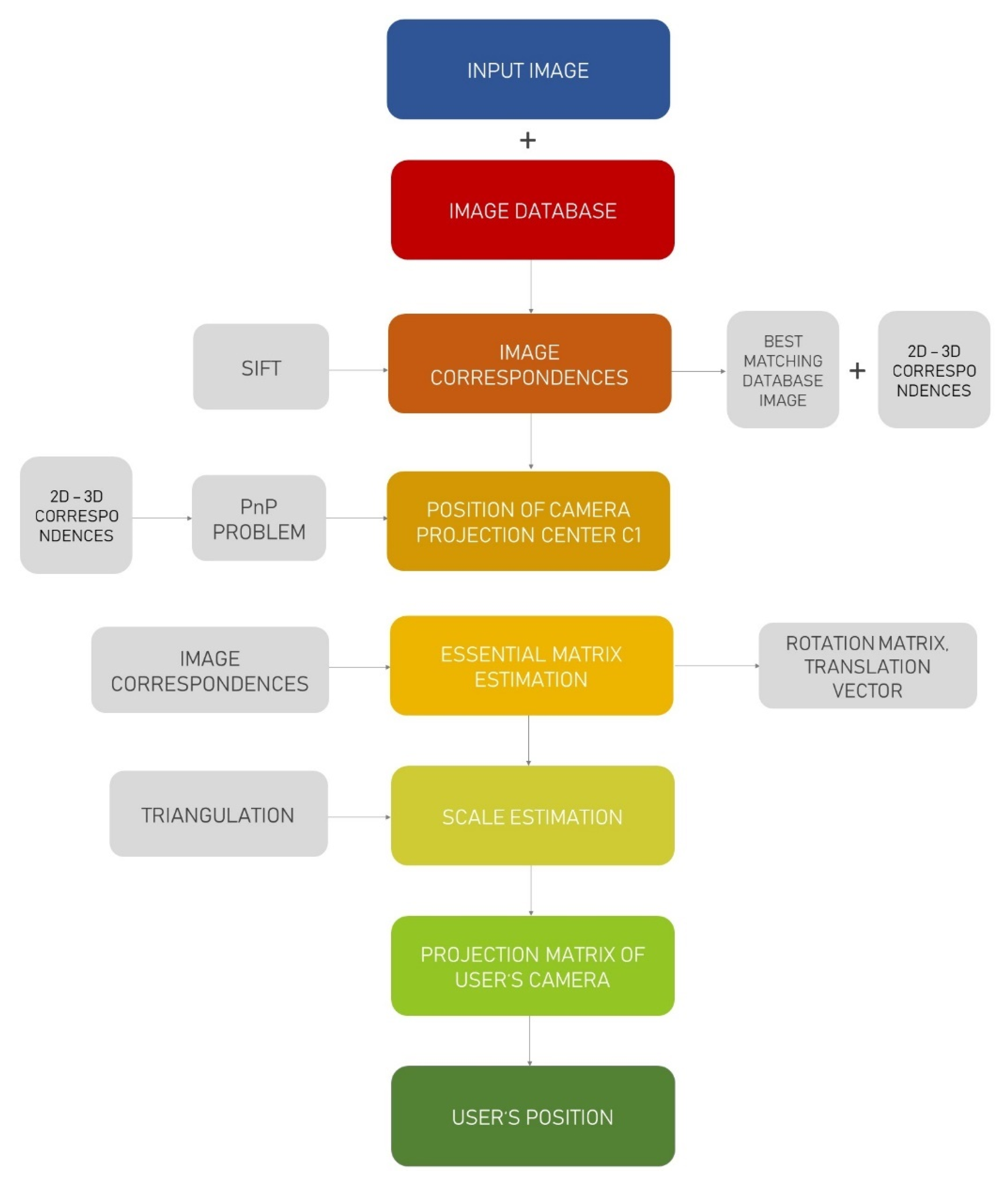
3. Designed and Implemented Solution
Database preparation consists of the following steps [
1,
2] see also
Figure 1:
- (1)
Surveying of the object coordinates (3D coordinates) of ground control points and taking an image of the interior space.
- (2)
Creation of the database of images with an XML description of each image in the database. Each XML image description consists of 3D ground control points coordinates and 2D coordinates of their images.
The rest of the process consists of a selection of the best matching image from the database to input image (input image refers to the image captured by user) using the SIFT algorithm and the user’s position estimation:
- (3)
Position of projection center of camera C1 (database camera position) estimation—PnP problem;
- (4)
Essential matrix estimation from features detected between input image and database image via SIFT;
- (5)
Estimation of the rotation matrix and translation matrix between the database image and the user’s image;
- (6)
Scale estimation;
- (7)
Projection matrix P2 of the user’s image estimation and user’s location estimation.
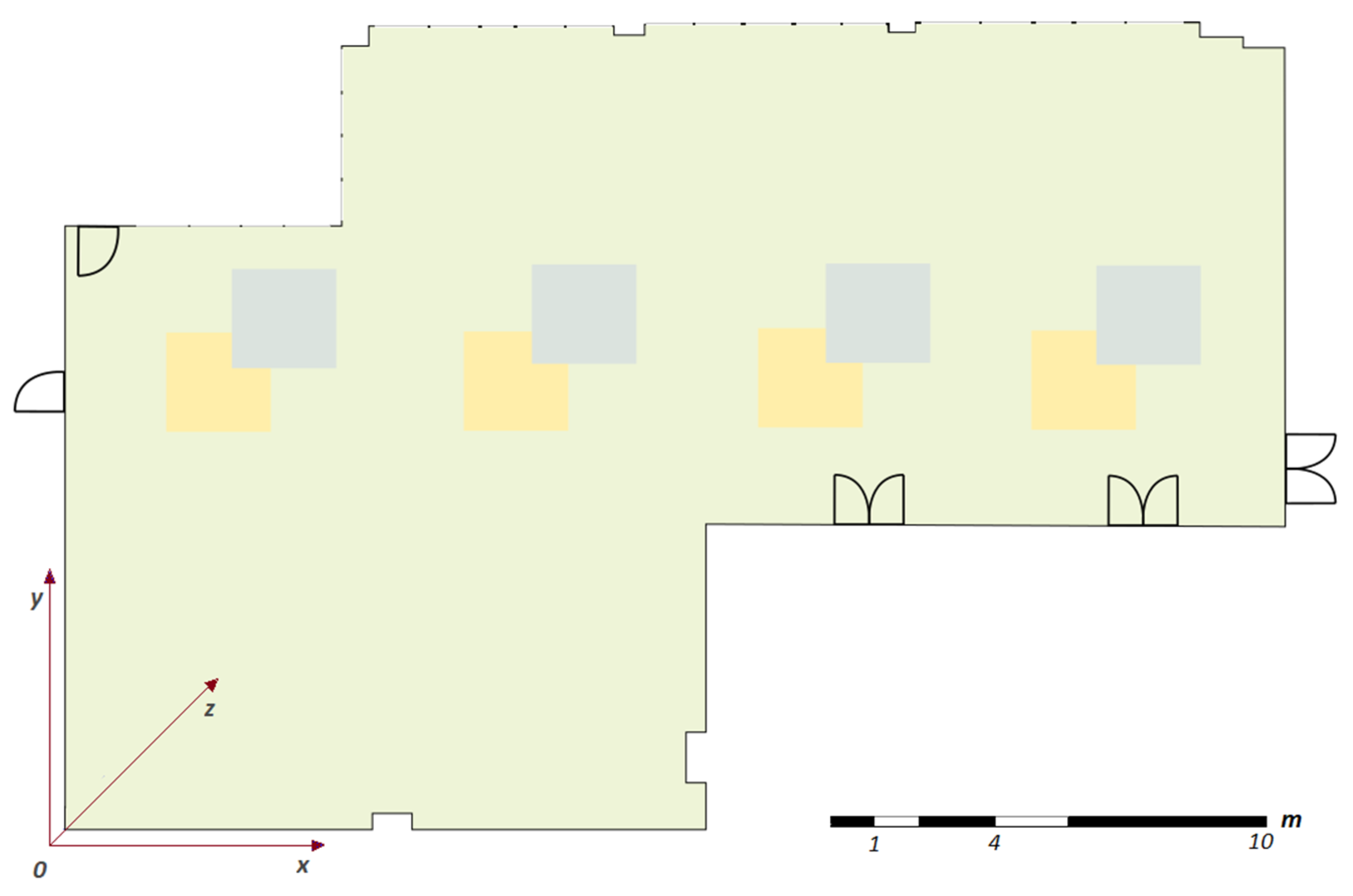
3.1. Database Preparation
The purpose of creating the image database is to obtain the reference position of the camera, which will be the basis for further user position estimation. For testing of our proposed solution, we use large office space (see
Figure 2).
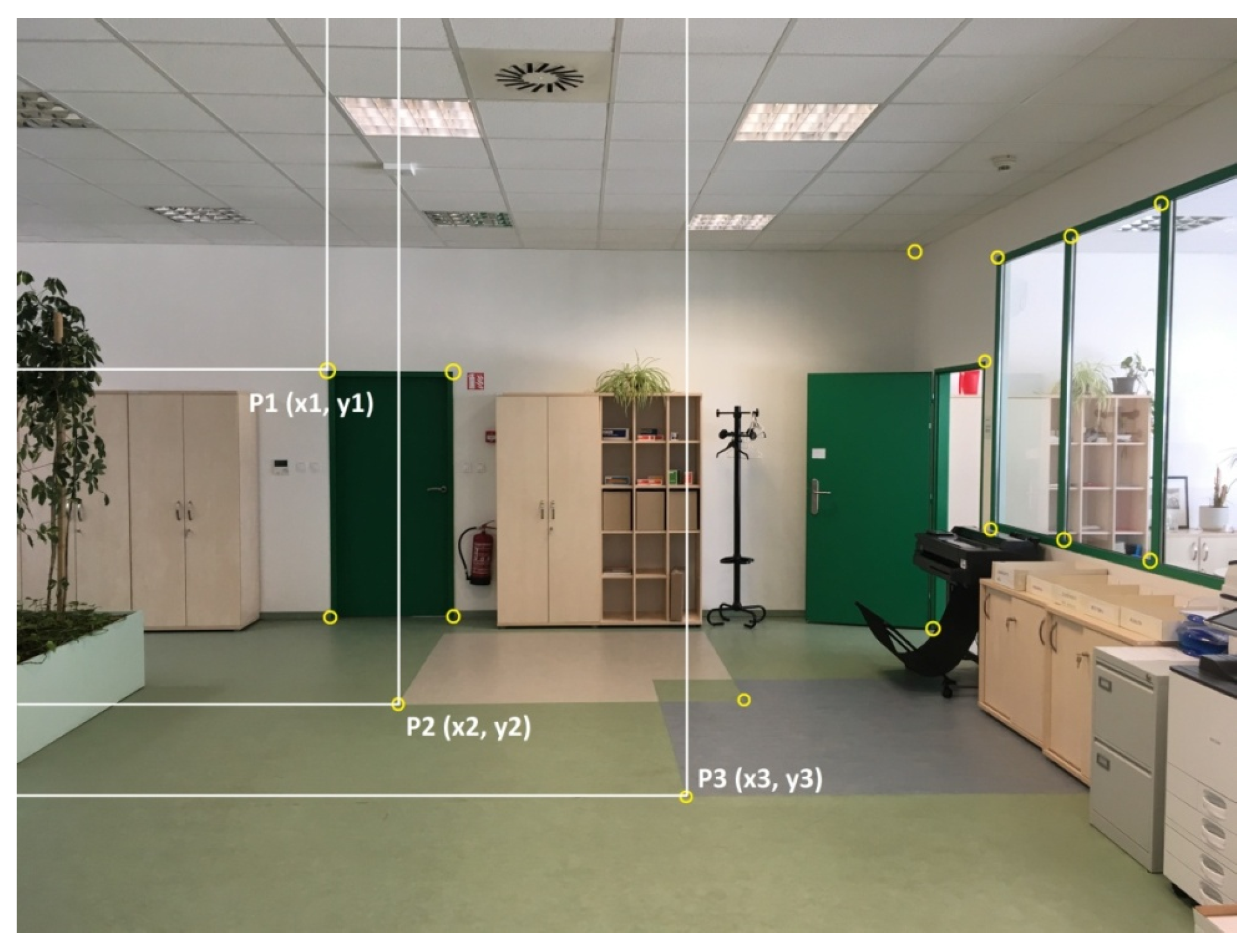
For the camera’s position determination via a single image, it is necessary to know at least six tuples. Ground control points were chosen to be invariant and well-signalized (corners of windows/doors/room or floor patterns). While selecting ground control points in the images, it was also essential to ensure that selected ground control points are not coplanar and are distributed as uniformly as possible (see
Figure 3).
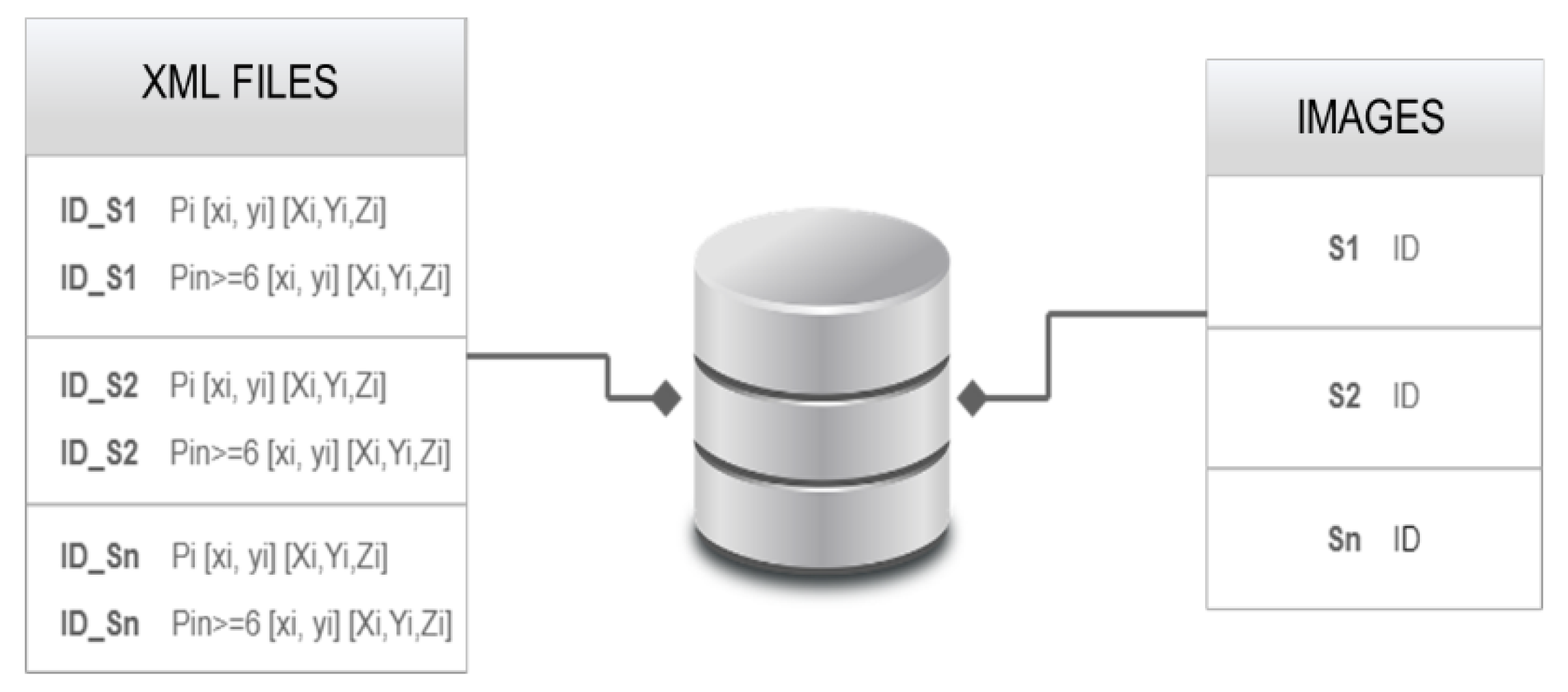
The database consists of an imaginary directory describing the office interior and associated XML files storing the tuples of 3D surveyed ground control points coordinates together with their 2D image coordinates (see
Figure 4). The interior of the building was photographed using an iPhone SE mobile phone camera, resulting in 60 images in total. All the images are taken from a similar height, which corresponds to real conditions, where the user holds its mobile device in hands while looking at the display.
3.2. Best Matching Database Image Selection
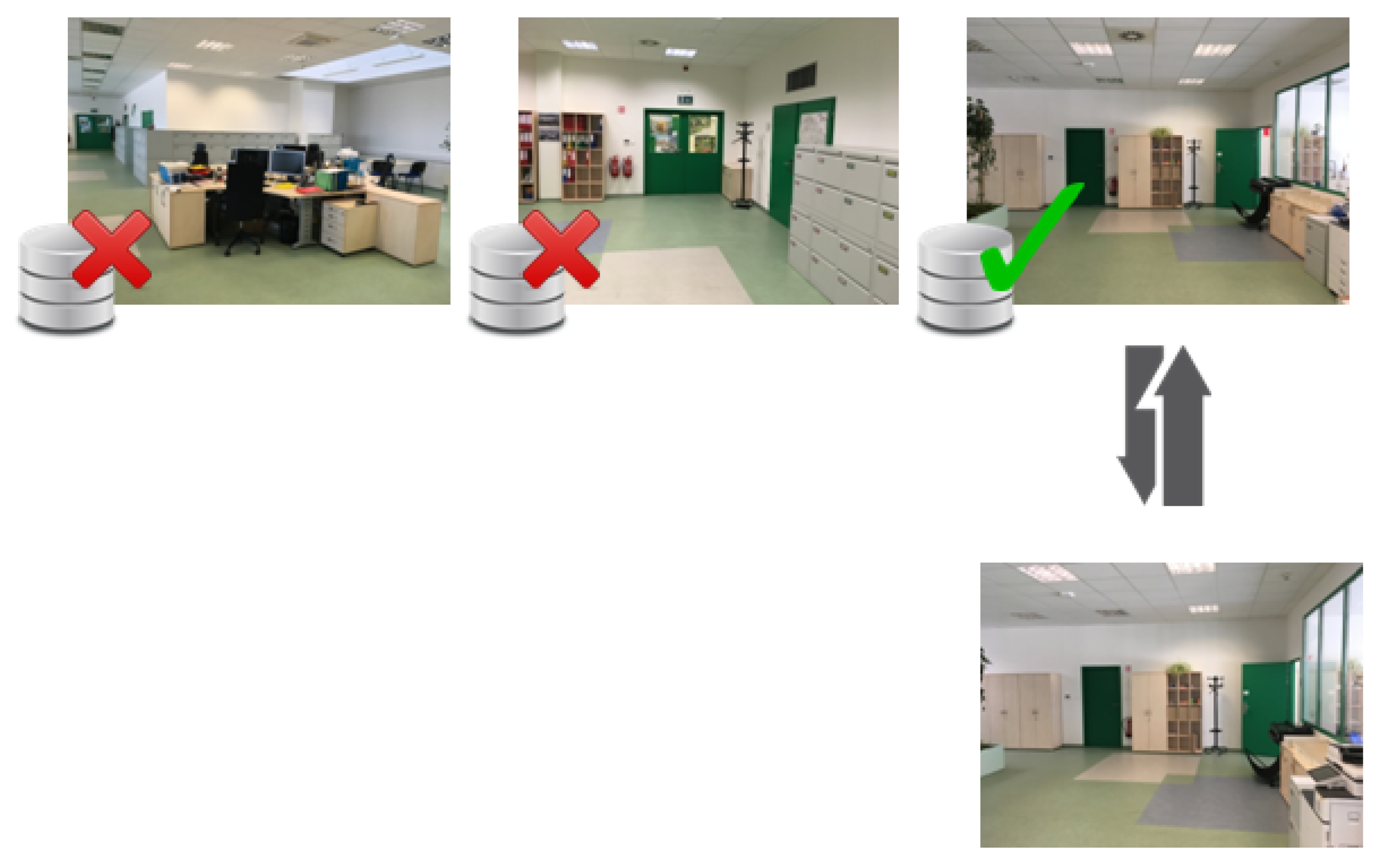
In order to select the best matching database image, we need to step through the image database, detect features (if the features of database images are not pre-detected yet) in all images, and assign correspondences between input image and database images. The best matching database image is the image with the highest number of possible correspondences retrieved (see
Figure 5).
The selection of a suitable feature detection algorithm is crucial for our work, because detected features not only have the function for searching for the best matching database image, but also play an important role in the estimation of the essential matrix. Although the computational speed of used algorithms is an important factor in the positioning process, it is more important to estimate the essential matrix from uniformly distributed and reliable detected and described features. For this reason, the SIFT algorithm was chosen for features’ searching.
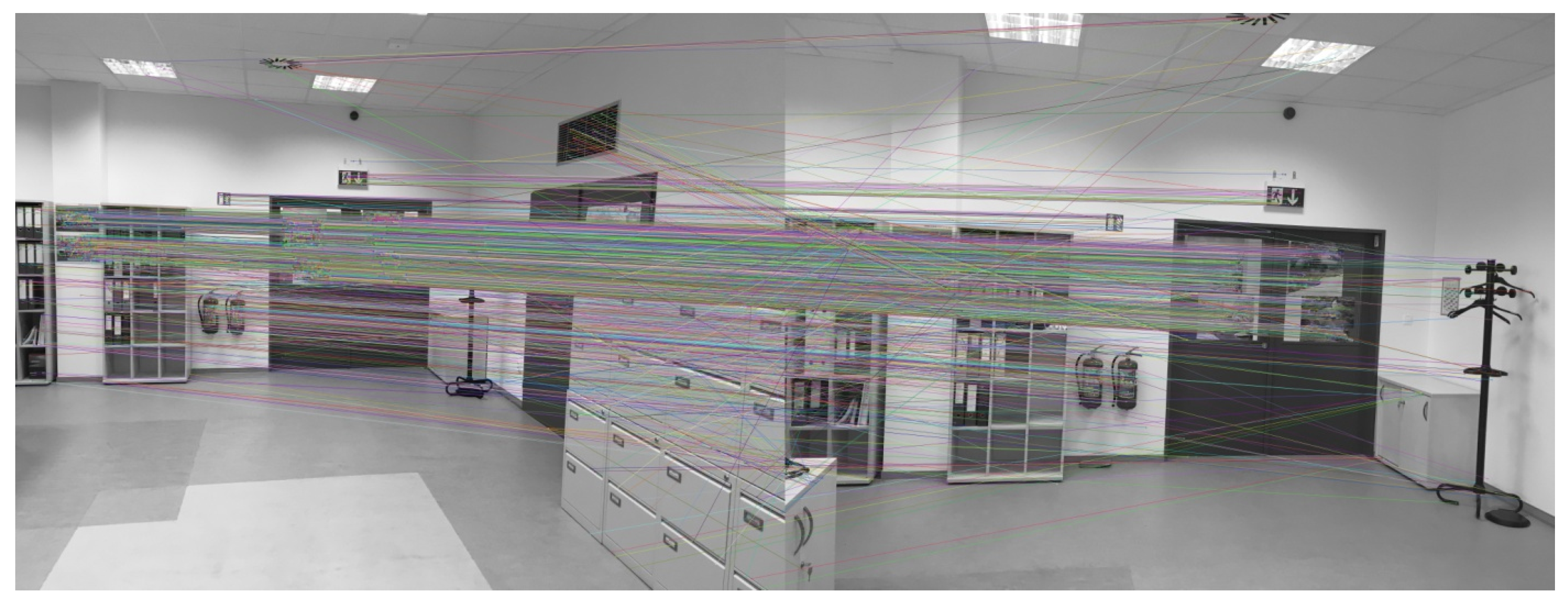
After feature detection and description, the next step is to find feature correspondences between input and database image (see
Figure 6). Based on the work of [
40], we used the FLANN-based matcher technique, which performs quick and efficient matching using the clustering and search in a multi-dimensional space module.
3.3. Essential Matrix E Estimation
Having found the best matching database image and feature correspondences, we can proceed to the calculation of the fundamental matrix
, which will be useful later for essential matrix
estimation. As shown in
Figure 6, correspondences contain outliers. To remove outliers, the RANSAC algorithm is used. After fundamental matrix
estimation, we can estimate essential matrix
, whose decomposition gives us a rotation matrix
and translation vector
t describing the relationship between positions of camera projection center
and camera projection center
. Formula
shows that it is necessary to know the internal calibration elements of camera. Using a mobile phone camera, determination of internal calibration elements needs be carried out by calibration process. An Agisoft Lens [
41] using a pinhole camera model for camera calibration was selected for this purpose.
After obtaining the values of essential matrix estimation, the next step is SVD decomposition of the essential matrix. However, SVD decomposition provides two possible solutions for the rotation matrix and two solutions for the translation vector t. Combining two solutions for the rotation matrix and the translation vector t, we get four possible solutions for the projection matrix of the user’s camera. The way to find the right solution is a triangulation of image correspondence. If the triangulated point has a positive depth, i.e., lies in front of both cameras, the solution is considered as correct.
3.4. Projection Matrix P1 Estimation
Despite having the correct solution for the rotation matrix
and translation vector of the user’s camera relative to database camera, we cannot determine the user’s location (projection center of camera
) until we know the location of the database camera (projection center of camera
) in the object coordinate system. For database camera projection matrix
estimation, we use principles of the PnP problem. The necessary tuples for the PnP problem solution are stored in the XML file belonging to the database image. Having estimated the projection matrix of the database camera, we can extract the position of the database camera projection center
based on the given formula:
3.5. Scale Estimation
Despite having the correct direction of the translation vector
t, we encounter a fundamental problem. The estimated translation vector is unitary and we need to achieve its correct size. To reach the scale, we triangulate two ground control points having stored in our database image XML file. Using a pair of ground control points, it is possible to determine the distance of triangulated ground control points in the camera coordinate system. Let us call this distance
. Furthermore, their actual distance
in the object coordinate system can be easily calculated from 3D coordinates of control points. Finally, the resulting scale is determined using the relationship:
3.6. Projection Matrix P2 Estimation—User’s PositionEestimation
Finally, the projection matrix of the user’s camera can be estimated based on the following relationship:
In this case, the calibration matrix of user’s camera is the same as calibration matrix of database camera. After substituting all needed values into the above formula, we can extract the user’s position the same way as in the case of database camera projection center .
4. Results
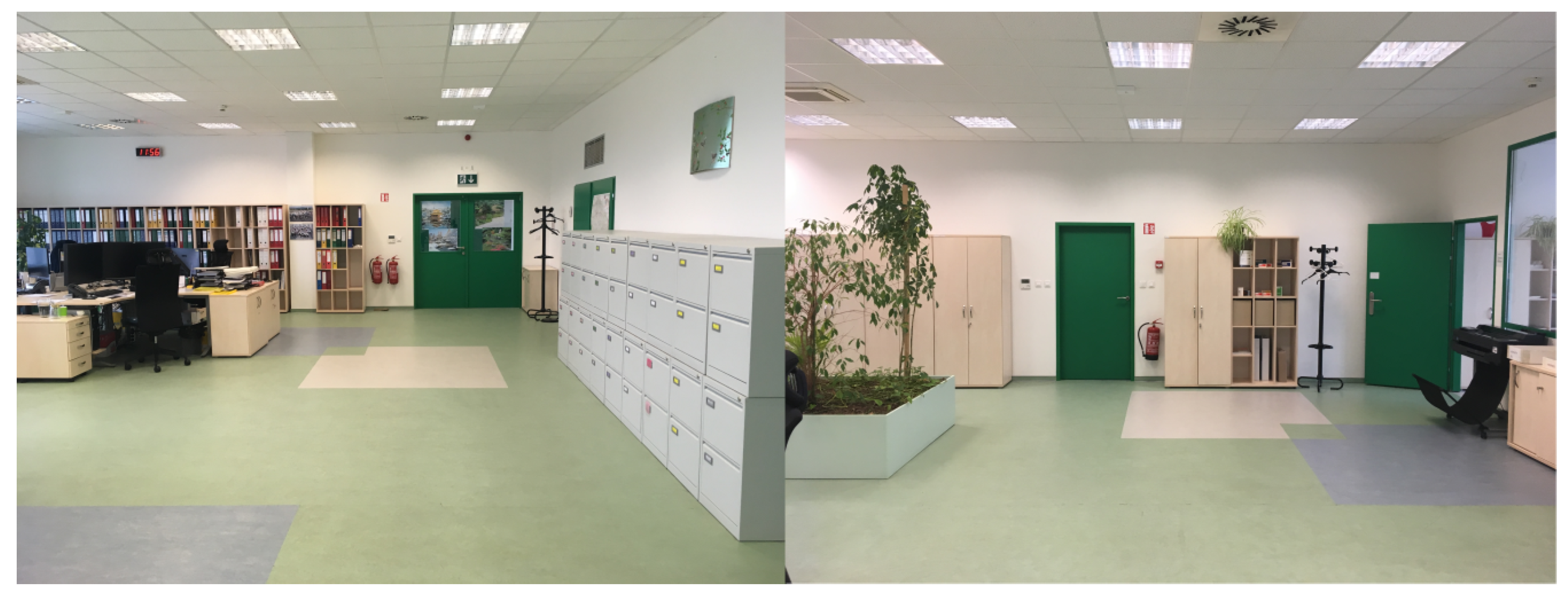
Our proposed solution was tested on two different views (see
Figure 7). Several constraints were applied in order to make the experimental work effective. The constraints were, however, designed in a way not affecting the tested results. First, it is worth to mention that the images were taken during ideal conditions, i.e., without movement of people in the captured scene, without change of the captured scene and with the same mobile phone camera that took the images into the database.
Next, some of the tested images were taken under lighting circumstances similar to images from the database. Therefore, in order to verify the resistance of the solution to photometric changes, several test images were taken at a lower light intensity (lights off), for which the positions of the projection centers were also estimated. These are IMG_5071, IMG_5072, IMG_5074, IMG_5082, IMG_5084, and IMG_5086.
Last but not least, a total of 12 input images were tested for view 1. Input images were tested against a set of 14 database images. For view 2, 5 input images were tested against a data set of 9 candidate images. It means that not the whole image database, but only the images with potential overlap were pre-selected from the image database, solely for faster calculation of the experiments, as processing the rest of the database would not find any true feature correspondences as they portray different areas of the room.
As mentioned above, the experiment started by searching for correspondences between the tested image and the database images. After finding the corresponding database image and estimating the user’s position, the pair of input image and database images was switched. It means that the best matching database image was used as an input image and the input image as the best matching database image. The assumption was that we obtain a very similar result for location error. Although our theory was confirmed in most cases, there were some significant location errors.
Table 1 shows that this problem applies to a pair of images 5 and 16. Despite a higher number of feature correspondences (2868) in pair number 5, we received a positioning error of 0.74 m. The higher value of the positioning error was caused due to wrong translation vector estimation. Wrong translation vector determination was noted, especially in cases where the length of the baseline between projection centers of cameras was very short, and the projection centers were almost identical. In the case of pair number 5, the baseline was 0.1 m long as well as for pair number 16. Such a case can be detected and excluded from an automatic positioning algorithm.
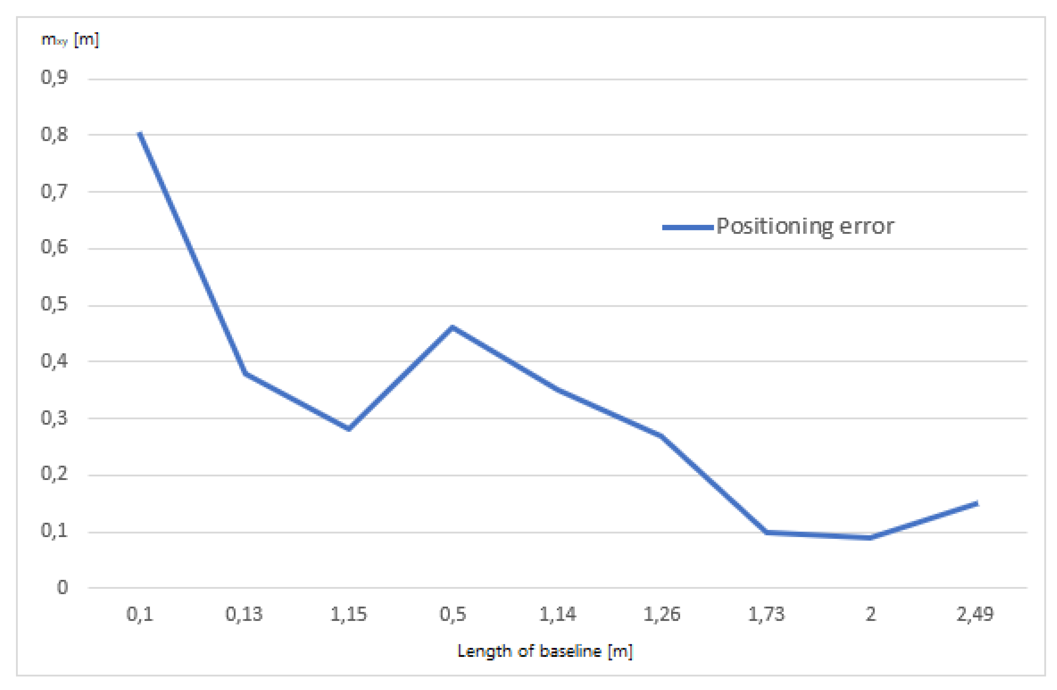
A short baseline (more precisely small baseline/depth ratio) leads to an increase in localization error because of sharp angles between optical rays in triangulation (see, e.g., [
42]). It is in conformance with our results. The values of mean coordinate errors in the
Figure 8 below confirm that the positioning error decreases with a longer baseline between projection centers of user camera and database camera. However, this problem can be easily overcome using another database image.
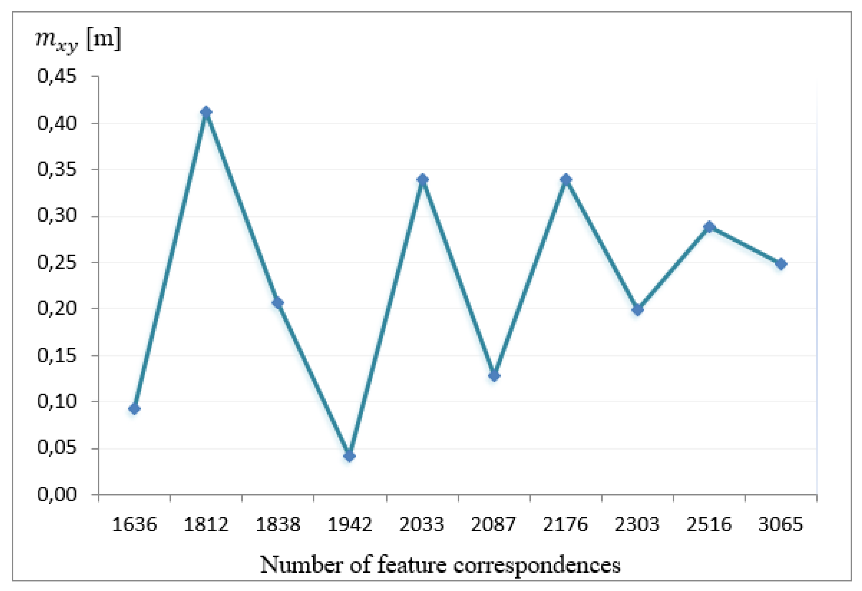
If we look at the number of feature correspondences found and the mean coordinate error in positioning, we find cases when positioning error is higher despite the higher number of feature correspondences. The fact that a higher number of feature correspondences does not always guarantee higher position accuracy led to another test of our proposed solution. The next test’s idea is to estimate the user’s position with a decreasing number of feature correspondences.
From the following results, it is evident that the number of retrieved feature correspondences does not affect the resulting positioning accuracy if the scene is the same. Based on the given results, the image database for view 1 was limited from the original 14 images to 5 images, and the test was performed again (see
Table 2 and
Figure 9).
Regarding feature correspondences, it was found that the position was determined with the positioning error up to:
0.1 m for more than 50% of tested input images;
0.20 m for almost 30% of tested input images;
0.50 m for the remaining 20% of input images.
Moreover, these results show significant insight. The lower the number of stored images in the database capturing the same scene of the interior, the higher the probability of accurate positioning. In other words, a low number of stored images in the database reduces the probability of retrieving the best matching image from the database with a similar projection center to the user’s camera.
Please note that larger baselines, leading to higher location accuracy, can be reached by taking the database images from unusual heights near a floor or ceiling.
5. Discussion and Further Research
As mentioned in chapter 1.1: Related Works, indoor localization is a problem with many possible solutions. It is still an open question, which solution will step outside of the academic ground to commercial life and become successful. We believe that the reason for the slow transition to wireless beacon localization is the need for new onsite infrastructure. On the contrary, our solution does not require any new physical infrastructure (only the virtual image database has to be created) and therefore, should prove to be easier to implement. Using a phone camera is a simple action that should not bother the user profoundly, and as was proven by the proof of concept experiment, the localization is reliable even with a tiny pool of database images. The rest of this section discusses the advantages and limitations of the designed core experiment in more detail.
First of all, we simplified the experiment design by using the same mobile phone camera for shooting both the input images and the database images. We have already had detected the internal calibration parameters of the given mobile phone camera using Agisoft Lens software. In real deployment, internal calibration parameters of mobile phones can be expected to differ. For this reason, a real user would need to find out the calibration parameters of his/her mobile phone before he or she wants to use the phone for such a localization.
Next, it was found that the most feature correspondences are found in image areas where regular patterns, pictures, or text characteristics occur. Although one of our tests showed the indirect proportion between the number of feature correspondences and positioning error, there could be an uninteresting scene (e.g., white walls) in terms of image processing. Such a scene would miss sufficiently contrasting features. The missing contrast could then result in a low number of feature correspondences and the impossibility of position estimation. It would, therefore, be appropriate to add pictures or text characteristics to an area of interest, as mentioned in [
24].
Also, the computation complexity should be discussed. The feature detection and description in a single image take approximately 3 minutes using hardware with the following parameters—1.8 GHz CPU, 2 GB GPU, and 6 GB RAM. The SIFT algorithm has a computational complexity of O(
n2), where
n is the average number of SIFT descriptors in each image [
43]. For this reason, the computational cost of the SIFT algorithm is another drawback of our proposed solution. In contrast to that, FLANN and RANSAC computing time together took a couple of seconds. Computational demands of the proposed solution could be reduced by having detected and described features stored in the database. Feature detection and description with the SIFT algorithm would be related to user-captured images only. Another solution for reducing the computational complexity could be the hierarchization of images based on an evaluation of how often is each particular database image used. Besides, in real-life deployment, the client-server architecture could be separated and thus requests for location estimation would be sent from the application to a web server equipped with more powerful hardware.
Next, localization accuracy and also reliability of the localization can be significantly increased by performing localization against several database images and merging the results altogether. Considering user movement constraints (speed of movement and space arrangement) allows preselection of database images and minimizes probability gross localization errors.
Last, but not least, the configuration of the building interiors and furniture could change over time. Some equipment may be moved, removed, or added. Such environmental changes would unfavorably affect the number of inlier feature correspondences between the database image and the input image. As a result, this would happen to inaccurate or even impossible positioning. The image database would, therefore, need to be updated in real use. A possible solution lies in a continuous update of the database where, once an image was successfully localized, it naturally becomes a part of the image database. However, such an approach would fail when significant changes in the interiors happen. Then, a remapping of the database would, of course, have to happen for the changing area.
6. Conclusions
To summarize, our contribution starts with a thorough discussion of relevant related works used for indoor positioning, talking of both infrastructure-based and infrastructure-free solutions of indoor localization. Also, the rising influence of methods based on artificial intelligence (neural network in particular) is shortly mentioned. However, at the beginning of the study, we decided to aim in the direction of using epipolar geometry, which needs a much lower level of scene understanding. Contrary to complex neural-networks-based approaches, which need to understand the perceived scene as a whole, our solution searches just for feature correspondences and then uses analytical geometric operations. Therefore, our solution (described in the Materials and Methods chapter) is more suitable for portable hardware such as a cell phone. It is, in fact, a common phone camera, that was used for the image capture. The camera’s position is then calculated in utilized contemporary software. The Results section then presents the accuracy achieved, and we found the sub-meter accuracy very promising.
Although this manuscript presents just the core experiment—a proof of concept that such a method can be used for indoor localization—we can imagine that the algorithms can be deployed into a client—server solution for real use. Many extensions of the core method would have to be developed to reach a real application. Therefore, the direction of further research and development is discussed in the Discussion chapter, and such a direction of research seems very promising.


