An Integrative Approach to Assessing Property Owner Perceptions and Modeled Risk to Coastal Hazards

Abstract

Coastal communities are increasingly vulnerable to changes in climate and weather, as well as sea-level rise and coastal erosion. The impact of these hazards can be very costly, and not just in terms of property damage, but also in lost revenue as many coastal communities are also tourism-based economies. The goal of this study is to investigate the awareness and attitudes of full-time residents and second-home property owners regarding the impact of climate and weather on property ownership and to identify the factors that most influences these attitudes in three coastal counties (Brunswick, Currituck, and Pender) of North Carolina, USA. The majority of previous studies have focused on only full-time residents’ risk perceptions. Given the fact that these coastal communities have a high percentages of second homes, this study fills that research gap by including second-home owners. This study integrates both social (survey data) and physical (geospatial coastal hazards data) aspects of vulnerability into a single assessment to understand the determinants of property owners’ risk perceptions and compare their perceived risks with their physical vulnerability. The study also compared the utility of a global ordinary least square (OLS) model with a local geographically weighted regression (GWR) model to identify explanatory variables in the dataset. The GWR was found to be a slightly better fit for the data with an R² of 0.248 (compared to 0.206 for the OLS). However, this was still relatively low and indicated that this study likely did not capture all of the factors that influence the perceptions of vulnerability in patterns of property ownership (whether full-time residents or second-home owners). The geospatial variables used to determine coastal vulnerability were found not to significantly impact perceptions related property ownership, but did provide additional insight in explaining spatial patterns of the response variable within each county.

1. Introduction

The coast of North Carolina is subject to severe weather events, erosion, and flooding in the low-lying coastal plain. This can be costly to state and federal governments and leave communities with infrastructure and property damage. The National Oceanographic and Atmospheric Agency (NOAA) annually calculates the cost of weather and climate related hazards (starting in 1980; [1]). Overall, the number (and total cost) of billion-dollar disasters is consistently increasing over time [1]. This is due to a combination of changes in the intensity and frequency of hazard events, as well as population growth in hazard-prone areas [1,2]. World-wide over 1 billion people live in these high-risk zones and that number is expected to grow [2]. In 2016, Hurricane Matthew alone cost state and federal governments approximately $97 million in financial assistance to those affected by the flooding [3]. More recently, 2018 was classified by NOAA as the fourth most costly year on record for hazards ($91 billion). This included Hurricane Florence that made landfall on the NC coast and cost an estimated $24 billion [1]. Overall, the Atlantic and Gulf coasts have exhibited an increase in tropical storm activity since the 1990s, leading to longer term impacts on both coastal communities and ecosystems [4,5]. These environmental risks contrast with the attraction of NC’s coastal communities to tourists and residents alike. This study seeks to ascertain what factors influence the perceptions of full-time residents and secondary homeowners regarding the effects that climate and weather risks have on property ownership.

Research suggests the importance of community member perceptions of climatic and weather-related risks, in addition to scientific knowledge and measurements of these risks [6,7]. This is due to risk perceptions associated with weather and climate influencing reactions to policy and decisions made at the local, state, and federal levels. These include: readiness to evacuate in case of storms, mitigation and preparation efforts, and fluctuations in property values.

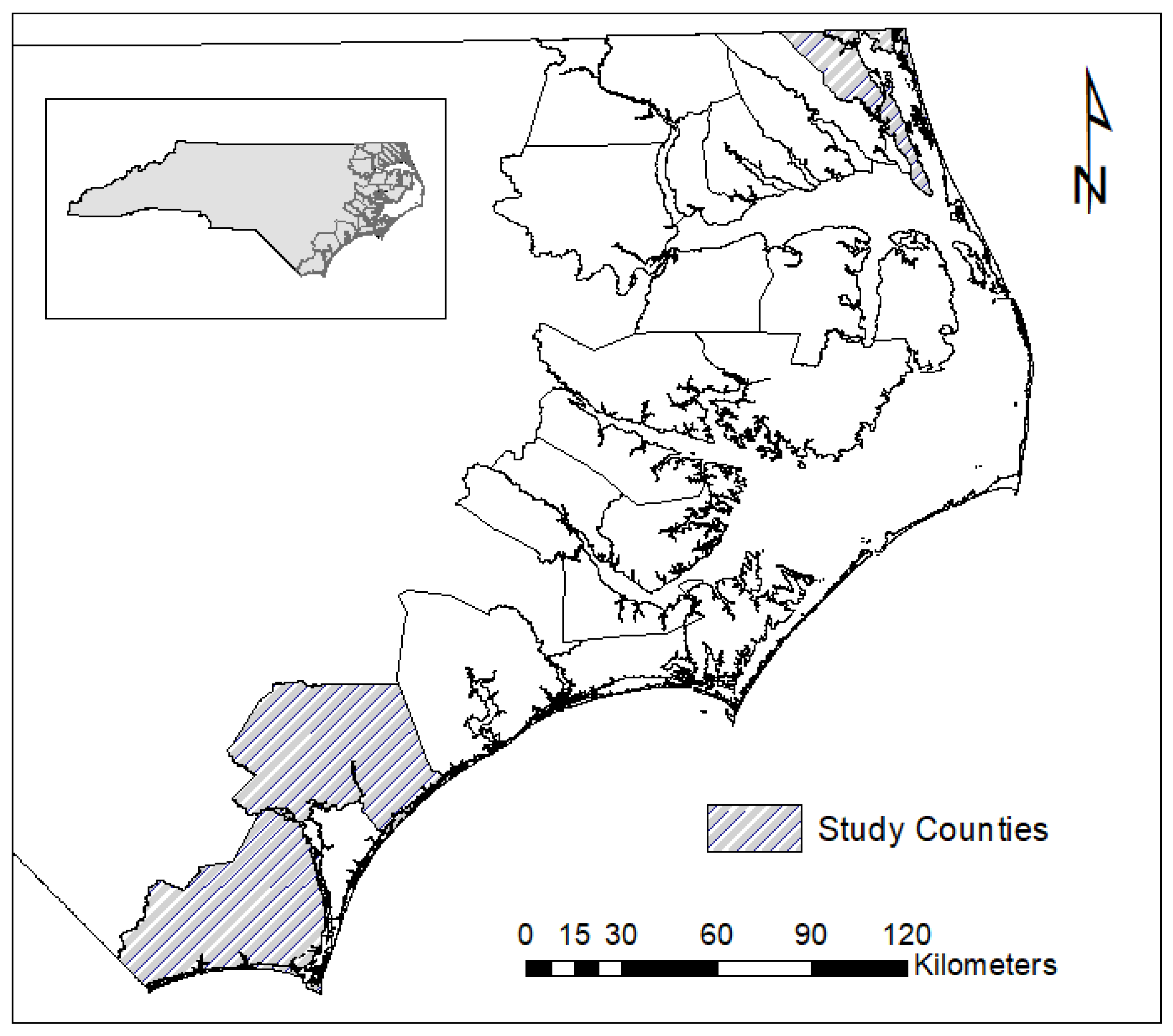
This study targets three high-amenity, tourist-based coastal communities in North Carolina: Brunswick, Currituck, and Pender counties (Figure 1). Because Brunswick, Currituck, and Pender counties have largely tourism-based economies, vacation homes make up a significant portion of property ownership. For instance, in Currituck County, secondary home ownership is 43% of the total home ownership in the county. Our study incorporates secondary homeowners into the sample (accounting for 53% of respondents), whereas previous studies have failed to collect survey data on this population. This represents a gap in many previous studies which have essentially not included almost half of the homeowners in some of these counties. Second home development and associated tourism also often impact decision making regarding the county’s economy, environment, and community culture. From a physical hazard perspective, these counties also represent a range of coastal conditions and morphologies across the state’s coastal zone. While weather and climate related risks can impact the entire coastal zone, these counties represent a range of common topography, barrier island morphology, and hydrologies, and therefore potential physical vulnerability to hazards [8].

1.1. Coastal Hazards

Coastal communities in NC are subject to multiple hazards that can impact local ecosystems, infrastructure, and the economy. This study focused on severe weather, flooding, and coastal erosion as the primary, and specifically near-term (temporal), risks to these communities. Long-term sea level rise was not addressed here due to the complexity of modeling those impacts on the coastal landscape. Additionally, the focus of this risk vulnerability assessment was to determine the current, not projected, vulnerability of coastal homeowners.

North Carolina coastal communities are subject to multiple tropical and extra-tropical storms every year [3,4,5]. Tropical storms are recognized as the costliest hazard (over $900 billion since 1980) and most deadly [1]. It is also the second most frequent hazard event. NC has experienced the second highest number of billion-dollar tropical storm events in the country (second only to Florida) over the last thirty years, costing over $400 billion in disaster recovery (adjusted costs; [1]). These impacts are only expected to increase over the next several decades. Tropical storms primarily impact coastal communities through flooding, either storm surge or precipitation-driven inland flooding. Both types of flooding were captured in the present study by utilizing storm surge models from NOAA and FEMA flood hazard maps. Storm surge flooding primarily impacts ocean and estuarine shorelines and is a relatively short-term, but high-impact event. Inland flooding driven by precipitation can last for weeks after the storm event and is often the most damaging and costly [1,3]. Additionally, flooding from both tropical and extra-tropical storms and other events has increased over recent decades in North Carolina [4,5].

Coastal erosion due to human activities and wind-driven waves was also examined as part of this study. Erosion rates from 0.5 to over eight meters per year has been documented across the east coast of the United States and in the coastal zone of North Carolina [8,9,10]. The average rate of erosion for estuarine shorelines in North Carolina is about 0.5 m yr⁻¹ while the average for some of our study area (lower Cape Fear River) is about 0.2 m yr⁻¹ [8,9,10].

1.2. Public Perceptions

Public risk perceptions of climate change and weather events are the focus of a growing number of studies ranging from climate science to sociology and real estate finance [6,7,11,12,13,14,15]. Much effort has gone into modeling the factors affecting these risk perceptions in different target groups, varying from United States citizens, Floridian homeowners, university students, and residents with direct experience of environmental hazards [15,16,17]. Six major factors influencing risk perceptions arise from previous studies. These include: (1) socioeconomic status, (2) demographics, (3) direct experience, (4) individual attitudes/beliefs, (5) the social context of respondents, and (6) location [13,15,16,17,18,19]. The factors and perceptions of risk are most commonly assessed by distributing quantitative surveys [13,15,16] or by conducting semi-structured interviews [17]. The inclusion of location-based variables, such as peak wind gust contours [13] or proximity to coast and elevation in the 100-year floodplain [15], have been modelled using geographic information systems (GIS) and compared with the respondent’s location. The extra dimension of physical risk determined through GIS modelling is useful to relating perceived risk with quantified risk.

Location serves an important role in risk perception. For one, it can relate back to the social context of a respondent in the form of sense-of-place or their emotional and community ties to a location. On the other hand, it can juxtapose respondent perceptions acquired through survey data with mapped risks in their corresponding areas. Location-based factors, such as location in high peak wind zones [13], the 100-year flood plain, areas threatened by sea level rise, and distance to coast [15], were often significant in explaining respondent risk perceptions, though not always in the expected direction. Although some of the measured environmental risks were associated with higher risk perceptions, living in the floodplain was negatively associated with perceptions of risk [15]. Additionally, proximity to coast as a predicting factor is inconclusive in its significance, having both significant and nonsignificant effects on an individual’s risk perceptions [15]. Physical risks from weather and climate generally impact the level of perceived risk.

This study is also unique in that it integrates both social and physical aspects of vulnerability into a single assessment. The majority of previous work in the area of coastal vulnerability has focused on either social or physical vulnerability, to the exclusion of the other. These studies also do not incorporate the perceptions of a population regarding their potential vulnerability to coastal hazards. Some limited work has been conducted in North Carolina that integrates homeowner perceptions with field measures. This was targeted to assess the relationship between perceptions of waterfront homeowners regarding shoreline protection methods to actual measures of their efficacy when impacted by hurricanes [20].

The goal of this study is to investigate the awareness and attitudes of property owners regarding the impact of climate and weather on property ownership and identify the factors that most influence these attitudes. This study integrates both social (survey data) and physical (geospatial coastal hazards data) aspects of vulnerability into a single assessment to understand the determinants of property owners’ risk perceptions and compare their perceived risks with their physical vulnerability. Figure 2 outlines the overall study methodology for integrating social and physical vulnerability and the utilization of both OLS and GWR models.

Based on the discussion above, the following research questions are raised:

• Question 1: What factors influence property owners’ perceptions of climate and weather’s positive effect on property ownership?
• Question 2: Do spatial effects exist in assessing property owners’ perceptions of climate and weather’s positive effect on property ownership?
• Question 3: Does the GWR model produce more accurate prediction than the OLS model and thus improve statistical fit?

2. Materials and Methods

2.1. Survey Data Collection

A random sample of full-time resident and second-home property owners were selected from the geographic information system (GIS) tax records from each county’s housing stock. The sample contains 7192 second-home property owners and 7395 full-time property owners. Second homeowners were defined as those who own property in the study area, but this property is not their primary residence.

The data collection was initiated by sending out an invitation letter to members of the sample and inviting them to visit the project’s website, enter a designated code number, and complete the survey. Participants also had the option of completing a hard copy of the questionnaire or answering the survey through a telephone interview. Two reminder postcards and two reminder phone calls were made to those who had not completed the survey, thus a total of five contacts were made during the data collection period. Thirteen hundred and ninety-three (1393) usable questionnaires were completed (53% second homeowners and 47% full-time residents). All data collection was conducted to the standards of the Institutional Review Board for human subjects research.

The survey asked questions related to the six factors shown in the literature to influence risk perceptions. Firstly, socioeconomic and demographic factors have repeatedly been found to have significant impact on a person’s perception of risks or willingness to address these risks [7,13,15,19]. Common predicting factors include: gender, race, and the economic status of the respondents. Higher risk perceptions are consistently associated with: women, minority groups, lower economic statuses, and lower education attainment levels [15]. However, additional studies also show an inverse relationship between age and risk perceptions [13]. Incorporation of these factors into the model is necessary for predicting risk perceptions.

Experiential factors in risk perception analysis refer to the direct exposure of an individual to a target environmental hazard. The effect of prior experience on risk perceptions is inconclusive. In the case of one study, it was found to be non-significant in their model [9], but in a study of Floridian homeowners, experiencing hurricane damage was a significant factor in predicting the level of perceived risk [13].

One aspect of climate and weather-related risk perceptions that has been incorporated into recent models is that of respondent attitudes and beliefs towards the environment and climate change. Attitude towards the environment is a significant predicting factor of environmental related risk perceptions. In two studies, attitude was determined using the new ecological paradigm (NEP), a measurement of an individual’s level of pro-ecological worldview, and respondent scores were positively related with increased perceptions of climate or weather-related risks [15,16].

Similarly, this theme has been measured in a variety of other ways, from affect, one’s preexisting disposition to an idea, and values [15] to measures of an individual’s perceived personal efficacy with regards to climate change [15]. These have provided some measure of an individual’s disposition towards climate change. In this study, attitude towards the environment is included through measures of sustainable actions and values, which provide a quantifiable measure of the respondents’ views towards sustainability and the environment.

The social context of respondents addresses knowledge, interest, and desire to seek out new information as it is transferred among social circles, as well as place-based social-psychological characteristics [15,18]. This has an impact on knowledge flow and ties to the land and community, which in turn influence people’s views of the land and risk associated with it [18]. Bonding social networks limit knowledge flow from outside sources and bridging networks support it. Increased willingness to adapt to climate change is associated with lower bonding social capital and higher bridging social capital [18]. This relationship is further explained as the interest of the respondent’s social network is a significant contributing factor to risk perceptions, as increased interest is related to higher perceived climate change risk [15].

Sense-of-place and social-psychological place-based dependencies had significant associations with perceived climate resiliency [18]. However, community and place-based ties are often overlooked in many of the climate change risk perception models. Other place-based factors, such as length of residency [13], have been included in previous studies but the emotional and social- psychological impact is not as universally addressed. This study incorporates sense-of-place factors into its model of climate and weather risk perceptions. The responses to questions under these six factors were then assessed using factor analysis.

2.2. Measurement and Factor Analysis

Property owners’ perceptions on how climate and weather affect their property ownership were captured in the survey by statements using a 5-point Likert-type scale (1 = strongly disagree; 2 = disagree; 3 = neither agree nor disagree; 4 = agree; 5 = strongly agree). These statements include: (1) Weather and climate conditions were important in deciding to own property in this County, (2) I feel the climate conditions here are ideal to attract new property owners, and (3) I feel I am adequately prepared for a severe weather event (e.g., hurricanes, floods, heavy rainfall). Principal component analysis (PCA) was conducted to assess the underlying dimension of the statements. One single dimension emerged, which explained 56% of the variance (

Table 1. PCA for Property Owners’ perceptions of climate and weather effects on current property ownership.

Dimension and Factored Items	Factor Loadings
Cronbach’s Alpha: 0.518; KMO: 0.730; sig.: 0.000; VE: 56%)1
Weather and climate conditions were important in deciding to own property in this County	0.708
I feel the climate conditions here are ideal to attract new property owners	0.718
I feel I am adequately prepared for a severe weather event (e.g., hurricanes, floods, heavy rainfall)	0.447

¹KMO—Kaiser-Meyer-Oklin; VE—Variance Explained

). The Kaiser–Meyer–Oklin (KMO) measure of sampling adequacy statistic was high (0.73) and the Bartlett’s test was significant (p = 0.000), suggesting the PCA analyses were necessary and appropriate. An average scale was computed and served as dependent variable.

Gender, age, duration of property ownership, annual household income, and education level data helped to understand the demographic characteristics of the respondents. Age was categorized into 10-year intervals, with the exception of the first two and the last groupings: 25 and under, 26 to 34, and 75 and over. Education level contains six categories: (1) less than high school; (2) high school or GED; (3) 2-year college or technical school; (4) some college, but no degree; (5) 4-year college; and (6) postgraduate. Annual household income was coded into ten categories ranging from 1 (less than $15,000) to 10 ($400, 000 and over). Duration of property ownership was determined based upon the number of years a respondent resided (for full-time residents) or owned a second-home property (for second-home owners) in the community.

The property owners’ community sense-of-place was measured by the following statements using a 5-point Likert-type scale ranging from 1 (strongly disagree) to 5 (strongly agree): (1) I feel that I can really be myself here; (2) I really miss it when I am away too long; (3) this is the best place to do the things I enjoy. The KMO statistic was 0.703 and the Bartlett’s test was significant (p = 0.000), suggesting that the principal component analysis was necessary and appropriate. All of the three items have factor loadings higher than 0.8 (

Table 2. PCA for Property Owners’ Sense of Place effects on current property ownership.

Dimension and Factored Items	Factor Loadings
Cronbach’s Alpha: 0.823; KMO: 0.703; sig.: 0.000
I feel that I can really be myself here	0.795
I really miss it when I am away too long	0.859
This is the best place to do the things I enjoy	0.839

). Reliability analysis produced a high Cronbach’s Alpha value of 0.823. A sense-of-place score was then created from the three items based on the strong reliability and used in the regression model.

To examine property owners’ perceptions on how climate change considerations affect property values, the authors used a 5-point Likert-type scale ranging from 1 (not at all) to 5 (to a very great extent) for the following statements: (1) changes in precipitation; (2) changes in temperature; (3) availability of freshwater; (4) number and intensity of coastal storms; (5) sea level and coastal flooding. Changes in precipitation and the amount and intensity of freshwater are highly correlated with the other three statements, hence they were later removed from the regression model.

Respondents were also asked their opinion regarding the importance of fifteen sustainable actions (See

Table 3. Principle Component Analysis for property owners’ perceptions of the importance of sustainable development in their community.

Figure	Factor Loadings
Cronbach’s Alpha: 0.920; KMO: 0.920; sig.: 0.000; VE*: 49%)1
Reducing and managing greenhouse gas emissions	0.759
Managing, reducing, and recycling solid waste	0.735
Reducing consumption of freshwater	0.694
Managing wastewater	0.792
Being energy efficient	0.826
Purchasing from companies with certified green practices	0.766
Training and educating employees on sustainability practices	0.753
Conserving the natural environment	0.725
Protecting our community’s natural environment for future generations	0.745
Protecting air quality	0.794
Protecting water quality	0.757
Reducing noise	0.601
Preserving culture and heritage	0.654
Providing economic benefits from tourism to locals	0.447
Full access for everyone in the community to participate in tourism development decisions	0.557

Note: * VE means Variance Explained.

) on the future economic success of their community’s tourism industry using a 5-point Likert-type scale ranging from 1 (not at all important) to 5 (very important). Sustainable actions were derived from the literature [21,22,23,24]. PCA was conducted and revealed a single dimension among these fifteen items which explained 49% of the variance as shown in Table 3. The KMO statistic was 0.92 and the Bartlett’s test was significant (p = 0.000), suggesting that the principal component analysis was necessary and appropriate. All of the fifteen items have factor loadings higher than 0.5. Reliability analysis produced a high Cronbach’s Alpha value of 0.92. A sustainable action score was then created from the fifteen items based on the strong reliability.

2.3. Coastal Vulnerability Index

An index of coastal vulnerability (CVI) was calculated in the software program ArcGIS 10.3.1 using public domain data from several online sources. Index variables and rankings are synthesized in

Table 4. Explanation of index values for storm surge, flood, and erosion risk. Storm surge index values derived from inundation by storm category. Flood risk index values derived from FEMA floodplain zones. Erosion risk index values derived from the USGS Atlantic Coastal Vulnerability Index data layer.

Index Value	Storm Surge Risk	Flood Risk1	Erosion Risk
1 – Lowest risk	Cells only flooded under category 5 conditions	Zone X – cells outside of 500 year floodplain	1
2 – Low risk	Cells flooded under category 4 & 5 conditions	0.2% change – cells in the 500 year floodplain	2
3 – Medium risk	Cells flooded under category 3–5 conditions	Zone A – cells with a 1% annual chance of flooding	3
4 – High risk	Cells flooded under category 2–5 conditions	Zone VE – cells in coastal areas with a 1% or greater chance of flooding; or at risk of storm wavesOrZone AE – cells in the 100 year floodplain	4
5 – Highest risk	Cells flooded under all storm surge scenarios (categories 1–5)		5

¹ Due to limitations of the source data, the flood risk index only has values between one (1) and four (4).

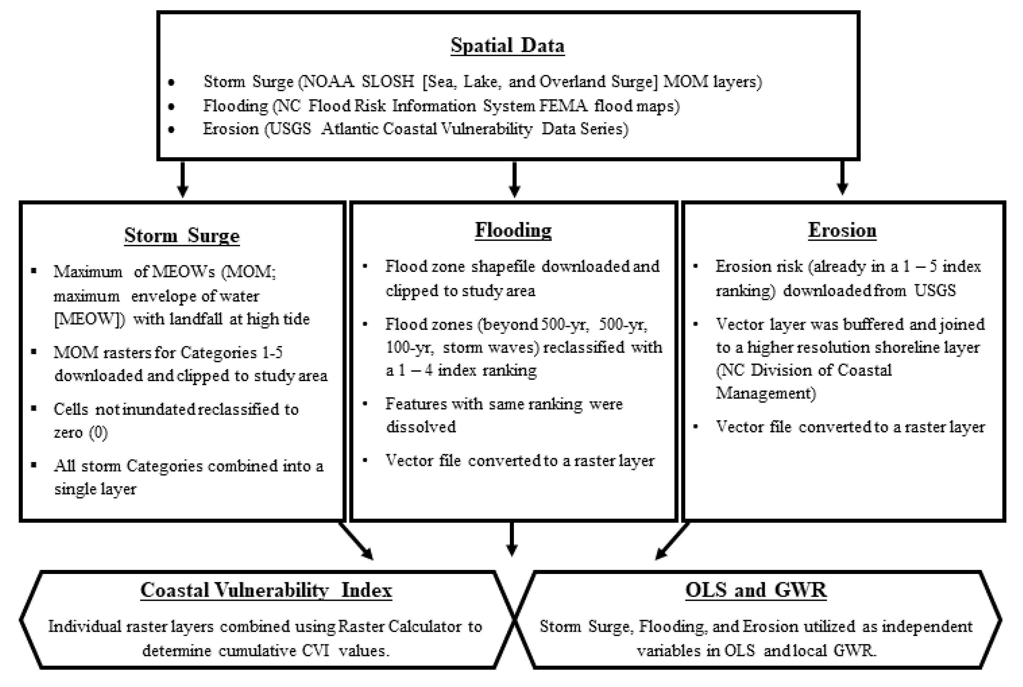
. Figure 3 illustrates the work flow for processing the spatial data layers used in the CVI calculation. Storm surge data was sourced from the National Oceanographic and Atmospheric Agency’s (NOAA) sea, lake, and overland surge (SLOSH) model. SLOSH uses a composite approach to efficiently provide forecasts of possible storm surge risk. All outputs are referenced to the North American Vertical Datum of 1988 (NAVD88) and represent water level above the reference datum. SLOSH basin outputs are updated every few years. The reported accuracy for projected storm surge from SLOSH is 20%. To assess the highest possible risk from storm surge, the maximum of the MEOWs (MOM; maximum envelope of water (MEOW)) with landfall at high tide was selected for analysis. The MOM raster for each category of hurricane (Categories 1–5) was downloaded for the Atlantic coast and clipped to North Carolina in ArcGIS. Raster cells not inundated under any storm surge scenario were reclassified to a value of zero (0). They were then combined to make a single combined storm surge layer. In this raster, a field was added to rank the extent of inundation on a scale from 1 (low) to 5 (high). Any coastal area subject to flooding in all storm categories (1–5) was ranked a 5, since these areas experience flooding during every hurricane, regardless of the hurricane’s strength. Areas that only experience storm surge during the strongest storm (category 5) were ranked a 1, since these areas are farther inland and do not flood during weaker hurricanes.

Data for the flood layer came from the North Carolina Flood Risk Information System at http://fris.nc.gov/fris/Download.aspx?ST=NC. This data consists of FEMA flood maps for each county. In the portal, you can select the county that you want data from and download as a shapefile. Once the data is unzipped, select V_E_FLD_HAZ_AR – this is the shapefile that will have the flood zone information in it. The field ZONE_LID_V contains the flood zone information that you will use to determine risk rating (1–3). Data was ranked from 1 to 4 based on chance of inundation, whereby 1 was low risk (outside the 500-year floodplain), 2 was medium risk (within the 500-year floodplain), 3 was medium-high risk (within the 100-year floodplain, no base flood elevations calculated), and 4 was high risk (coastal areas with base flood elevations calculated and additional hazard associated with storm waves). After merging all three county shapefiles, the feature class was dissolved by flood zone information (zone_lid_value). Then, a field (Flood_Index) was added to rank the polygons and the vector file converted to a raster using the cell size from the SLOSH data. Finally, a flood zone field was added to keep the FEMA flood zone data associated with the index ranking.

Erosion risk data was obtained from the Atlantic Coastal Vulnerability Index from USGS Digital Data Series (https://pubs.usgs.gov/dds/dds68/htmldocs/data.htm). This coastal vulnerability index already had erosion risk values from 1–5 associated with the shoreline, with 1 being the lowest risk of erosion to 5 being the highest risk of erosion (field: ERRRISK). Because this layer was at 1:2,000,000 it was buffered to a smaller scale shoreline and joined to provide a more detailed layer of erosion risk. It was then converted from a vector layer to a raster with a cell size of 100.

These three index variables: SLOSH, flood risk, and erosion risk, were then combined using the Raster Calculator tool in ArcGIS to calculate final, unweighted, CVI values (Figure 3). The layers were also utilized as independent variables in both an ordinary least squares regression model and a local geographically weighted regression model.

2.4. Ordinary Least Squares (OLS) Regression Model

Global regression models, such as ordinary least squares (OLS) regression, are the most commonly used methods to examine factors influencing people’s risk perceptions. This paper investigates the relationships between the dependent variable (property owners’ perceptions of climate and weather’s positive effects on property ownership) and a range of independent variables such as changes in temperature and/or humidity, availability of freshwater, sea level and flooding, demographic characteristics, sense of place, sustainability perceptions, slosh, erosion, and flood index. The study first uses OLS to explore the factors influencing property owners’ perceptions of climate and weather’s positive impacts on property ownership and assess the global relationship between the dependent variable and independent variables, then applies a geographically weighted regression (GWR) to capture the local varying relationships across the study area. The global regression models mask spatial heterogeneity in the relationships between the dependent variables and a set of independent variables and fail to consider the existence of local variation due to spatial autocorrelation [25]. To better understand the determinants of risk perceptions and how the relationships can be affected by location variations, the geographically weighted regression (GWR) model was adopted to investigate the effects of local factors on property owners’ risk perceptions. The GWR model allows estimated parameters to vary across the study area to accommodate potential spatial dependence [26].

OLS model performance is based on the following assumptions: (1) the relationships between dependent and independent variables are linear; (2) the observations in the dependent variable are independent of one another; (3) the data are normally distributed; (4) there is no multicollinearity among independent variables; and (5) the variance of residuals is the same across all values of the independent variables (homoscedasticity) [27]. Multicollinearity was assessed through the values of variance inflation factor (VIF) statistics, which measure redundancy among explanatory variables. Explanatory variables associated with VIF values larger than 7.5 suggest that they measure the same concepts and provide similar information. These variables were removed one at a time from the model based on VIF value until the multicollinearity problem disappeared. The examination of other assumptions for the multivariate regression analysis showed: (1) linearity between dependent and independent variables; (2) independence of observations in the dependent variables; and (3) normality.

The Koenker (BP) statistics (=144.86) is significant (p < 0.01) indicating the relationships modeled are not consistent, either due to non-stationary or heteroskedasticity. Hence, the assumption of homoscedasticity was violated and a spatial model such as GWR is necessary. Regression models with statistically significant nonstationarity are good candidates for GWR analysis.

2.5. GWR

Under conditions of non-stationary in OLS modeling, GWR was adopted to potentially fix the spatial autocorrelation problems and improve the model fit. Using the same dataset and the same explanatory variables as the OLS model, a GWR model was developed and performed following auto-calibration in ArcGIS. In contrast to estimations using a global model whereby one global R² was produced, the GWR local model produced a total of 1393 local regressions, wherein each of the regressions corresponded to one of the 1393 sample points. The condition index was below 30 (range from 23 to 26) for each local regression, indicating that the models did not have collinearity issues and the results are reliable. Additionally, a check for spatial autocorrelation using the Moran’s Index test was also conducted on the standard residuals for the GWR model. Moran’s index was significant (P < 0.05, z-score = 3.45, and Moran I = 0.33) and supported the reliability of using the local GWR model.

3. Results

3.1. Comparing Homeowner Perceptions with Physical CVI

Survey participants in three NC counties (Brunswick, Currituck, and Pender) were asked to express their views on how climate change factors affect their future property ownership. Almost 70% of the property owners felt that weather and climate conditions were important in deciding to own property in their county. Approximately 76% of the respondents agreed or strongly agreed that climate conditions in their county were ideal to attract new property owners. More than 70% of the survey participants (72%) felt they were adequately prepared for a severe weather event. These results indicate that overall, most property owners in the study counties felt comfortable with the current climate and weather conditions and felt they were prepared for any severe weather that they might encounter as residents of coastal NC.

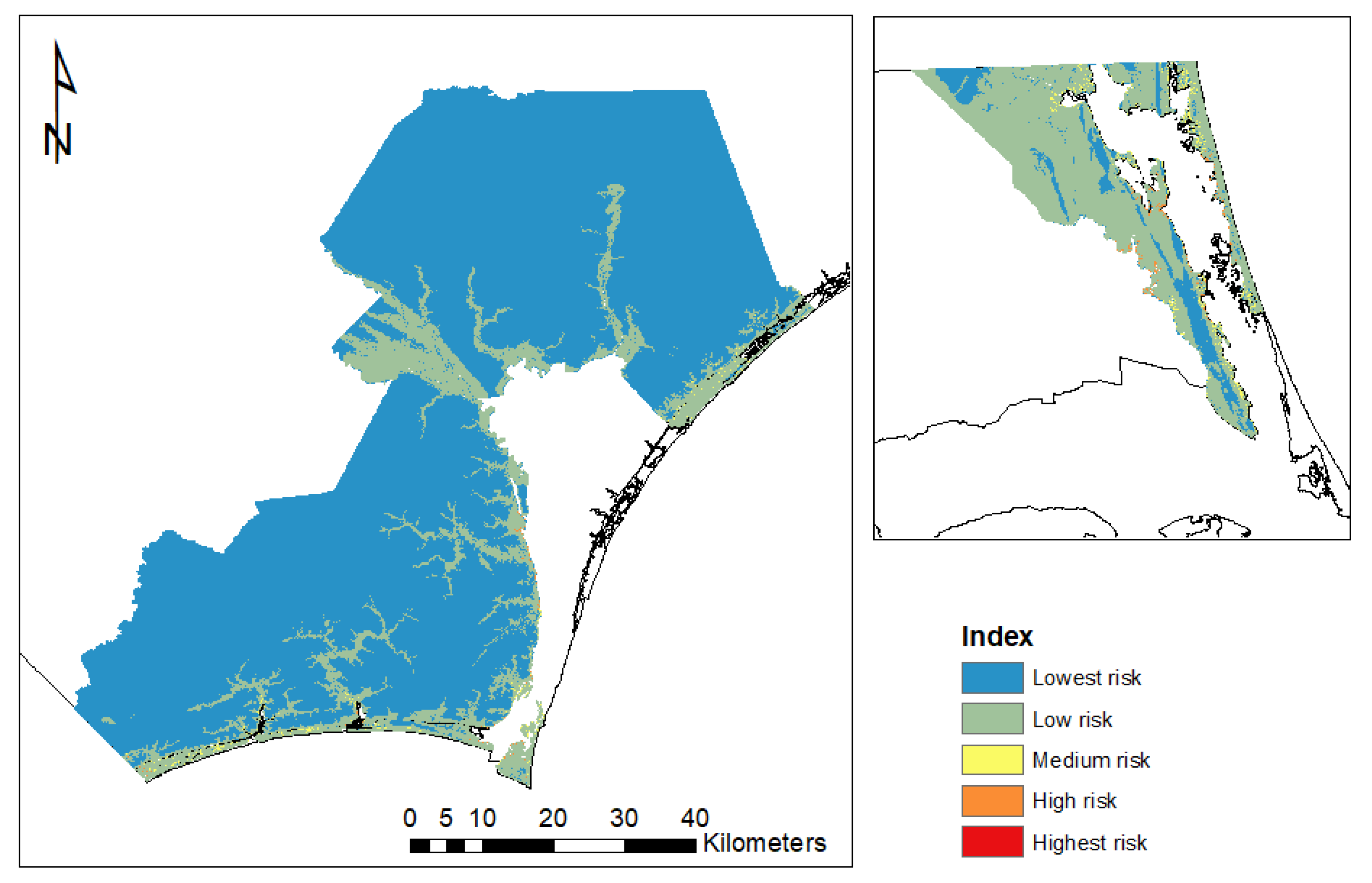
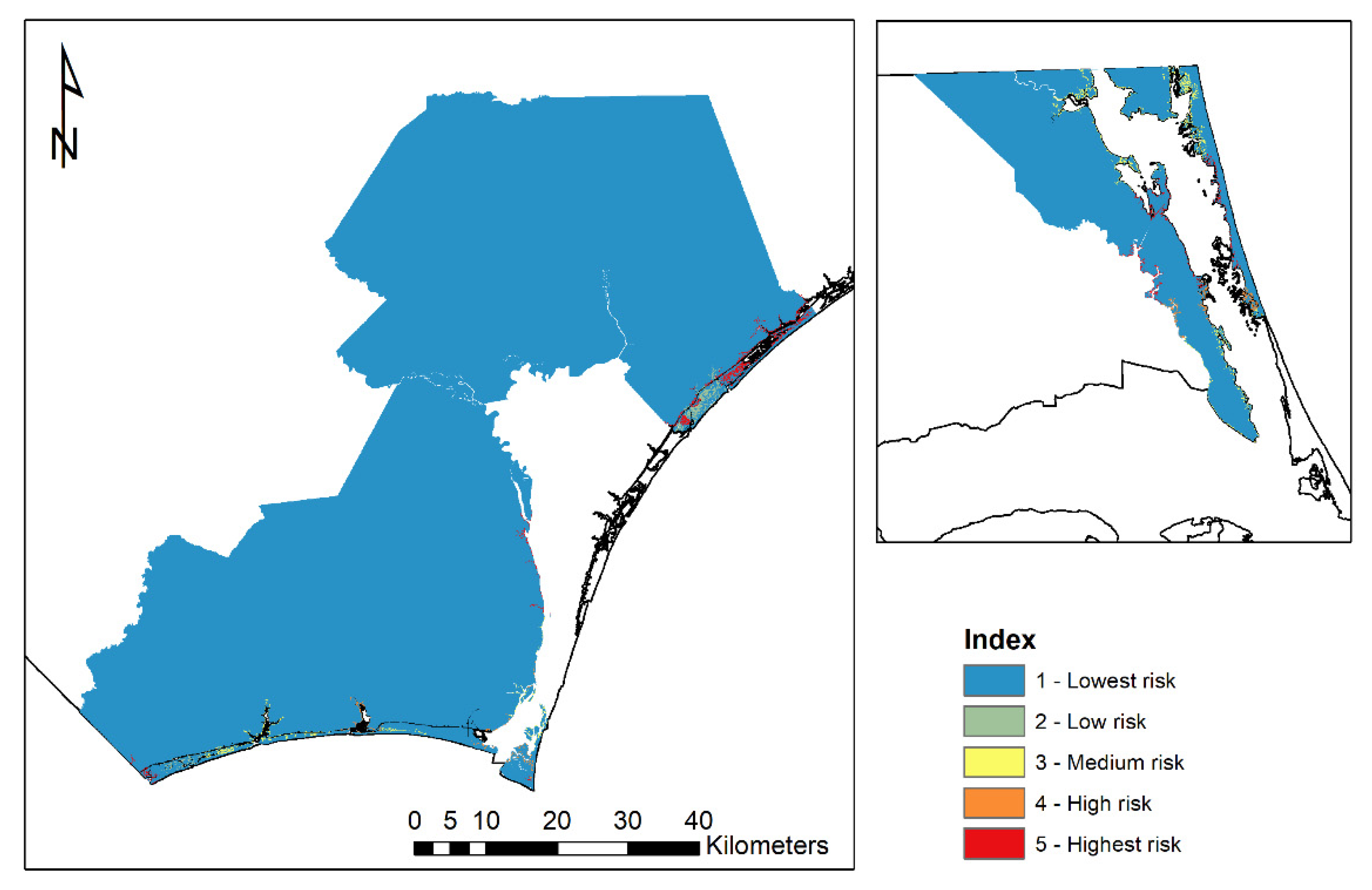
The majority of land area in the three counties of interest was determined to fall in the Low to Medium risk categories for the cumulative CVI (

Table 5. Percentage of area by county in each CVI risk classification.

CVI Classification	Brunswick County	Currituck County	Pender County
Lowest (1–3)	86.31	17.0	88.01
Low (4–6)	5.5	29.9	6.9
Medium (7–9)	7.9	50.41	5.1
High (10–12)	0.2	2.0	0.1
Highest (13–14)	0.1	0.7	0

¹ Greatest percentage of land area.

; Figure 4). For Brunswick and Pender counties, over 80% (86.3% and 88.0%, respectively) of total land area was in the Low risk category. In contrast, Currituck County had the highest percentage of land area (50.4%) in the Medium risk category, indicating the county is potentially more vulnerable to coastal hazards (Table 5). Only a small percentage of total land area in any of the counties was in the High to Highest categories. While only 0.1%–2.7% of these counties were determined to be highly vulnerable, these locations coincide with high-density, high-value development, and tourist amenities, such as public beachfront or other water access points. The majority of land are in these categories is concentrated along the barrier islands and estuarine shoreline (Figure 4). This is best illustrated in Currituck county (Figure 4), where the greatest land area in the High and Highest categories was determined (2.7%). The county also had the greatest length of shoreline and most risk for erosion (

Table 6. Summary of index variables by county. Reported as risk category with the greatest percentage of land area (percentages noted in parentheses). NA designation under the Erosion risk category represents the percentage of cells that were located inland (not shoreline coincident).

County	Erosion	Flood	Storm Surge
Brunswick	NA (99.4%) Medium (0.3%)	Lowest (62.6%)	Lowest (6.9%)
Currituck	NA (96.5%) Medium (2.1%)	Medium (58.3%)	Highest (41.8%)
Pender	NA (99.3%) Medium (0.4%)	Lowest (63.8%)	Highest (2.9%)

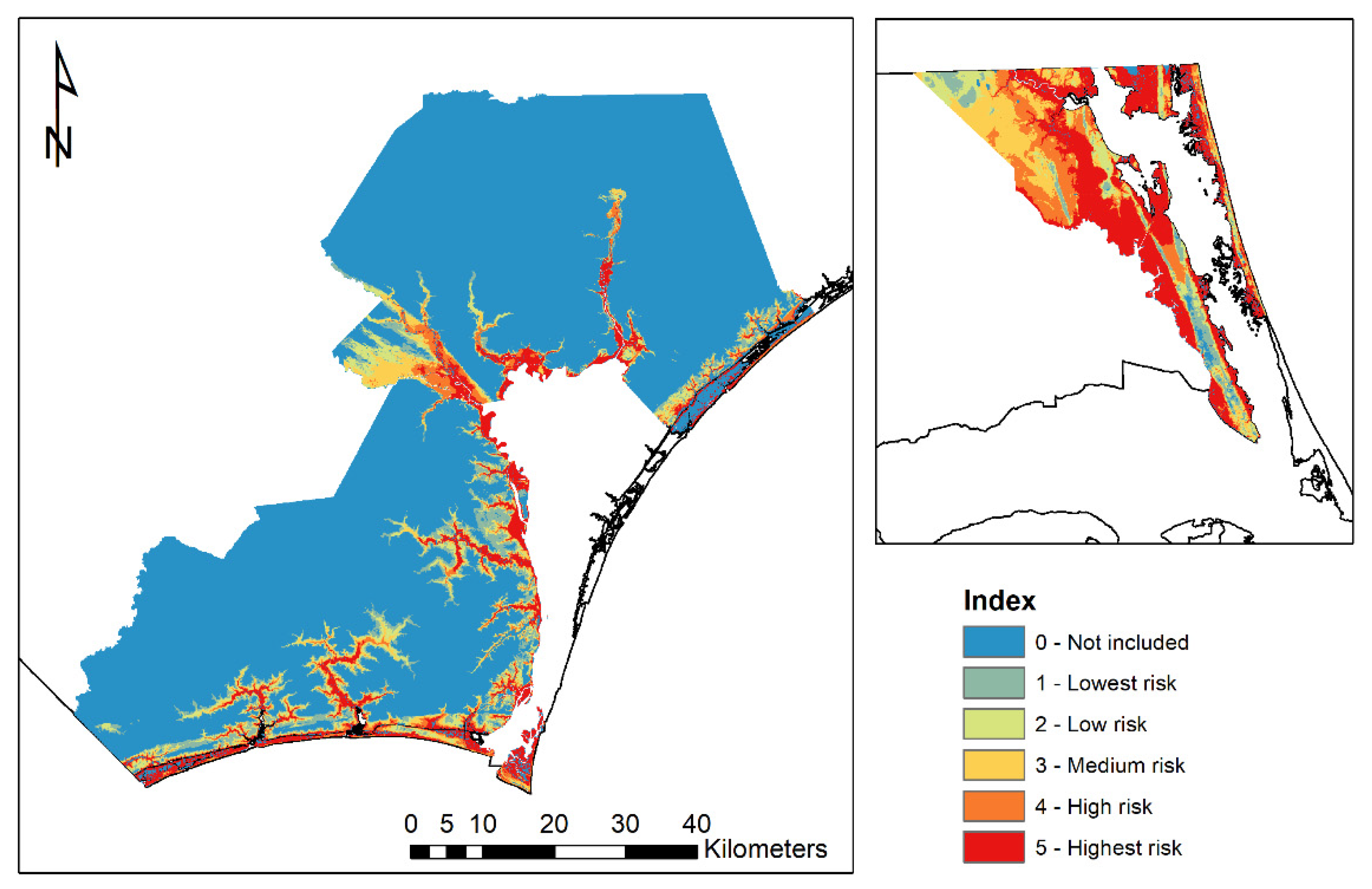
; [28]). When examining the contribution of each independent variable in the CVI (storm surge, flooding, and erosion), Currituck had the most land area in higher vulnerability categories for all three (Table 6; Figure 5, Figure 6 and Figure 7). It was also the only county in the study to have almost half of its land area (41.8%) fall in the Highest risk category for storm surge (Table 6; Figure 5). This is significant because of the extensive tourism present in the county. Currituck also has the highest percentage (43%) of second home owners compared to the other counties in this study, and a large number are present on the barrier island (part of the Outer Banks of North Carolina). Pender County also had some land area in the Highest storm surge category, but it only accounted for 2.9% of the county’s total land area (Table 6; Figure 5). However, like Currituck county, in Pender (and Brunswick), the highest risk, especially for storm surge, is along the barrier islands which are significant for the local economy. The higher risk to Currituck is likely due to a combination of physical variables, such as the amount of shoreline, average elevation, and the hydrodynamics associated with storm tides [4].

The survey responses regarding climate change and the calculated physical vulnerability were then utilized in a global OLS model to understand how each of these variables (perception of changes in temperature & humidity, perception of sea-level rise & flooding, SLOSH surge level, flooding, and erosion) influenced patterns of property ownership in the three NC counties. The physical vulnerability variables were found to not influence the property owners’ perceptions and therefore patterns of ownership. They responded that they were prepared for weather conditions and were satisfied with climate characteristics. In contrast, the CVI results indicate that these counties have potentially high vulnerability to coastal hazards, especially in Currituck County. However, while a direct influence was not observed in the data, it is not unexpected to see that, when on average the physical vulnerability is low, homeowners also exhibit less concern for their potential vulnerability.

3.2. Comparison of Model Results

3.2.1. Global OLS

A global OLS model was utilized to understand how the independent variables of the survey responses and physical risk layers (CVI components of SLOSH, erosion, and flooding) influenced patterns of property ownership in the three study counties. Only a few of the independent variables were found to be statistically significant (P < 0.05;

Table 7. OLS results for the 14 independent variables.

Variable	Coefficient	SE	p-Value
Intercept	1.664725	0.124927	0.0000*
Changes in temperature and humidity	0.048727	0.020279	0.016385*
Availability of fresh water	0.027319	0.019118	0.153237
sea level and coastal flooding	−0.048337	0.018573	0.009348*
Residential status	0.022583	0.043677	0.605219
Gender	0.080752	0.038613	0.036672*
Age	0.040757	0.014051	0.003791*
Length of owning property	−0.000221	0.000338	0.513413
Income	0.007131	0.007045	0.311561
Education	0.043582	0.014569	0.002837*
Sense of Place	0.268724	0.0216	0.000000*
Sustainable Actions	0.125668	0.016534	0.000000*
Slosh Index	−0.018467	0.014885	0.214937
Erosion Index	−0.015688	0.033952	0.644129
Flood Index	0.007346	0.025332	0.77188

*indicate sig. at 0.05.

). Property owners reported that changes in temperature and humidity have a positive impact on property values so they will continue to own and purchase property in the area. They also perceived that future sea-level rise and coastal flooding could have a negative impact on their property values, indicating that they recognize that there is a potential risk associated with owning property in the coastal zone. While not statistically significant, it was also noted that respondents perceived that freshwater availability has a positive impact on property values. Other variables, such as gender, age, and education, all showed a positive impact on people’s perceptions of climate and weather effects on property ownership. Specifically, the population demographics for the respondents of over 55 (almost 70%), educated (over 62% have a college degree or above), and male (55%) recognized the role that climate and weather plays in determining property ownership. An individual’s sense-of-place and their use of sustainable actions also had a positive impact, so property owners who felt more attached to a place and saw the value in sustainable practices were also more likely to recognize the impact of climate and weather on property ownership. Finally, the physical index variables (slosh, erosion, flooding) were not found to be significant. So overall perceptions of property owners play a direct role in patterns of property ownership, while actual physical risk does not. This creates a potential disconnect whereby what people perceive is what determines their actions, not what may actually be physically happening.

This study also compared the results between two potentially distinct population segments, full-time residents and second-home property owners. The same global OLS model was run for both populations. The results are reported in

Table 8. OLS results for Full Time Residents and Second Home Owners.

	Full Time Residents		Secondhome Owners
Variable	Coefficient	p-vlue	Coefficient	p-value
Intercept	1.815	0.000	2.481	0.000*
Changes in temperature and humidity	−0.018	0.500	0.042	0.121
Availability of fresh water	0.032	0.181	−0.005	0.849
sea level and coastal flooding	−0.024	0.303	−0.028	0.279
Gender	0.083	0.098	0.055	0.277
Age	0.082*	0.000	0.000	0.986
Length of owning property	−0.005*	0.003	0.000	0.711
Income	−0.008	0.576	−0.018	0.223
Education	0.022	0.243	0.049*	0.047
Sense of Place	0.258*	0.000	0.246*	0.000
Sustainable Actions	0.118*	0.004	0.069	0.136
Slosh Index	−0.005	0.791	−0.010	0.610
Erosion Index	−0.038	0.538	−0.011	0.794
Flood Index	0.008	0.817	−0.019	0.544

*indicate sig. at 0.05.

. A t-test was conducted to examine the differences in full-time residents and second-home owners’ risk perceptions. The result showed a statistically significant difference between the risk perceptions of full-time residents and second-home owners. This supports the need to survey both populations of coastal homeowners. To better understand these significant differences, the factors influencing these risk perceptions were investigated.

The OLS model for full-time residents shows that 21.2% of the variance in full-time residents’ risk perceptions were explained by the model (R² = 0.212, F = 9.684, sig. = 0.00). As shown in Table 8 age, sense-of-place and sustainable actions have significantly positive relationships with full-time residents’ risk perceptions. More specifically, older people and residents who felt more attached to a place and saw the value in sustainable practices were also more likely to recognize the impact of climate and weather on property ownership. Length of owning property has a negative relationship with people’s perceptions of climate and weather effects on property ownership. So the longer the residents lived in the area, the less likely they were to recognize the impact of climate and weather on property ownership. This may have implications related to storm evacuations or the level of preparedness residence have for severe weather events.

The OLS model for second-home owners shows that 10.1% of the variance in second-home owners’ risk perceptions were explained by the model (R² = 0.101, F = 4.34, sig. = 0.00). The model was not as a good fit for explaining the relationship between risk perceptions and homeownership. As shown in Table 8, education and sense-of-place have significantly positive relationships with second-home owners’ risk perceptions. That is, second-home owners who have higher education level and saw the value in sustainable practices were more likely to recognize the impact of climate and weather on property ownership. Overall, these results indicate a potential difference in both the perceived level of risk and the response to that risk between full-time residents and second-home owners.

3.2.2. Local GWR

A local GWR was utilized (for the composite dataset including both full-time residents and second-home owners) to find a better fit model for the data and examine geographic trends in the response variable. The same independent variables from the global OLS model were utilized. The overall results from the local GWR match those of the global OLS model, however GWR exhibited greater sensitivity and a little better fit. Property owner perceptions regarding temperature and humidity changes had a similar positive relationship to ownership as seen in the OLS. However, there are more negative coefficient values for this variable then were seen in the OLS, particularly in Pender County. This may be a function of the lower population density in this county. Results for homeowner perceptions of freshwater availability were also similar to those of the OLS with the exception of more negative values, primarily in Currituck County where almost 50% were negative coefficients. So, while on average homeowner perceptions of freshwater availability did not adversely impact property ownership, in Currituck County there was more of a negative impact on ownership. This may be due to localized variables not included in this analysis. Currituck County is well-connected to the neighboring Virginia city of Norfolk, which has extensive problems with flooding, salinization, storms, and other coastal hazards. Norfolk is also considered a leader in proactive management of coastal hazards and is home to significant infrastructure to facilitate that management (i.e., a USACE regional office and the Norfolk Naval Base). Property owners in Currituck are likely more aware of these issues as a result of their proximity to Norfolk, as residents in much of the county receive all of their over-air television and radio news from Norfolk. This relationship likely also explains the negative relationship between homeowner perceptions of sea-level rise and flooding on property ownership, which is in contrast to the results from the OLS model.

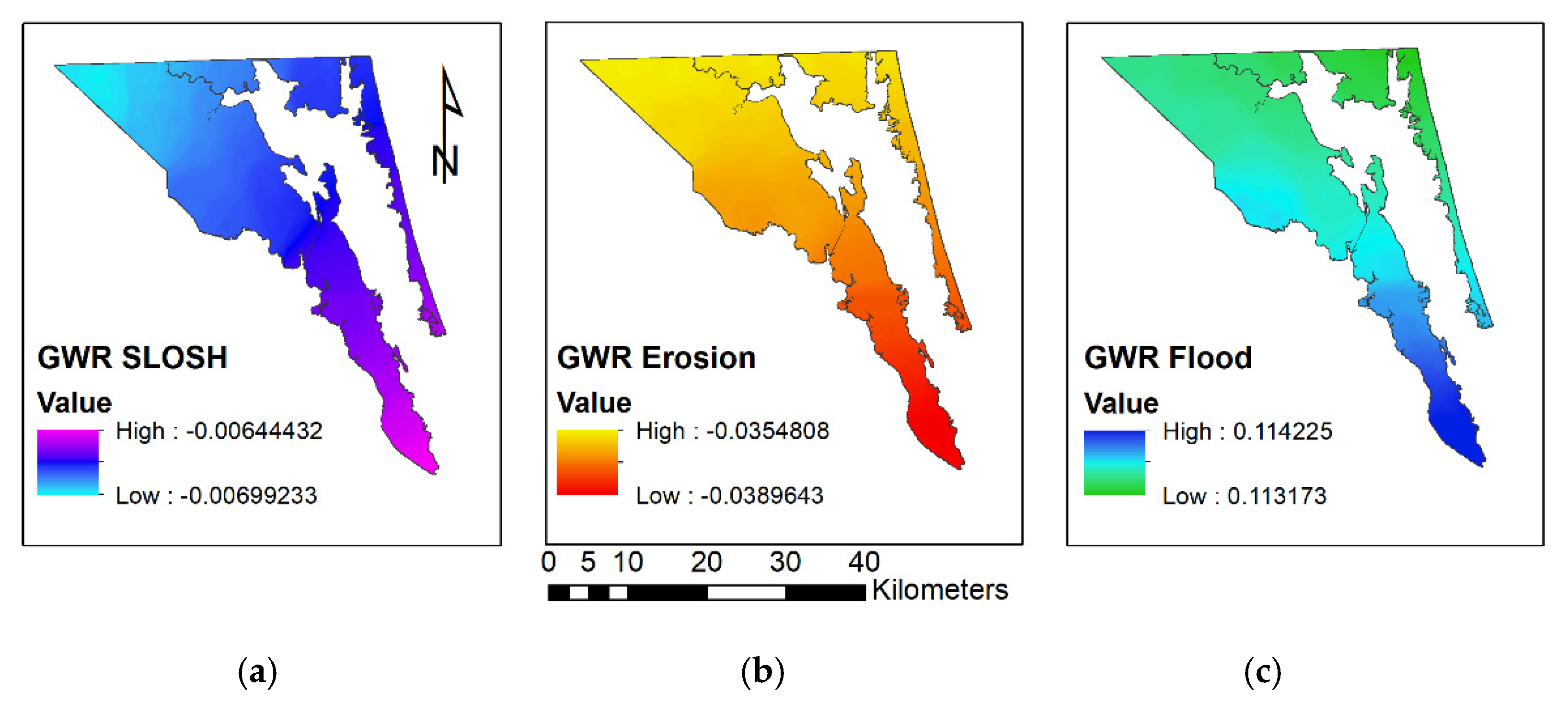
There are also clear geographic trends across Currituck County with the physical variables (Figure 8). The most negative coefficient values for storm surge and erosion are concentration along the southern shoreline of the mainland peninsula (Figure 8a,b), while the flooding variable show a positive influence on property ownership (Figure 8c). This may be due to the presence of Elizabeth City, the largest population center in the county, at this location. This may indicate concern for the impact of major storms, but some confidence in the city’s ability to handle other types of flooding. Overall, the GWR results for the three physical (CVI) independent variables showed similar results to the OLS model with the exception of Pender County where coefficients for the three variables were more negative.

3.2.3. Model Comparison

The comparison between the estimated results of the OLS model and the GWR was performed for the full data set (both full-time residents and second-home owners included). Various diagnostic parameters show the differences in performance between the OLS and GWR models.

Table 9. OLS and GWR model comparison.

	OLS Coefficients			GWR Coefficients
Variable	b	SE	p	Minimum	Mean	Maximum	Range
Intercept	1.664725	0.124927	0.000000*	1.390032	1.727093	2.372631	0.982599
Changes in temperature and humidity	0.048727	0.020279	0.016385*	−0.021457	0.048518	0.105747	0.127204
Availability of fresh water	0.027319	0.019118	0.153237	−0.020698	0.030291	0.080383	0.101081
Sea level and coastal flooding	−0.04834	0.018573	0.009348*	−0.06447	−0.04723	0.011807	0.076277
Slosh index	−0.01847	0.014885	0.214937	−0.05953	−0.00872	0.040956	0.100486
Erosion index	−0.01569	0.033952	0.644129	−0.147627	−0.04787	0.032936	0.180563
Flood index	0.007346	0.025332	0.77188	−0.175644	0.021135	0.114225	0.289869
Adjusted R square	0.206			0.222606	0.252763	0.354725	0.132119

shows the comparison of the performance of the GWR model and the OLS. Comparing the fit of the global OLS model assuming homogeneity of variables across the study area and local GWR model with no assumption of homogeneity, we found that the global OLS model produced adjusted R² value of was 0.206. The local GWR adjusted R² was 0.248, which suggests that there has been some improvement by using a local modeling approach. The other measure of model fit, AICc, gave a value of 2961 for the global OLS model and 2915 for the local GWR model. The difference of 46 is a relatively strong evidence of an improvement in the model fit to the data. Additionally, the problem of heteroscedasticity that was noted in the OLS model was not observed in the GWR model. Further, in the OLS global model, some predictors did not show any significant effects on property owners’ risk perceptions of climate and weather effects on property values, but did significantly relate to the risk perceptions in some specified area in GWR model, which indicates that the GWR model can achieve better performance. In particular, coefficients for the three physical variables were found to vary by county to a greater degree than was indicated in the OLS. Geographic patterns seen in these variables indicate the GWR model both performed better and led to a more comprehensive interpretation of the model results.

4. Discussion

This paper investigated factors influencing property owners’ perceptions of climate and weather’s positive effect on property ownership based on a sample of 1393 property owners in three North Carolina coastal counties using both the OLS and GWR model. The OLS model suggested that, in addition to common demographic variables (age, gender, education, etc.), respondent’s perceptions of the climate (temperature and humidity), freshwater availability, sea-level rise and flooding, sense of place, and sustainability were all found to influence patterns of property ownership in the three study counties. With the 14 available explanatory variables, the OLS model explained 20.6% of the variation in future property ownership perceptions and the residuals of the OLS model showed significant spatial autocorrelation, which indicated the limitations of the OLS model in explaining the property owners’ risk perceptions. In contrast to the global relationship established between the independent variables and risk perceptions by the OLS model, the GWR model captured spatial heterogeneity in explaining the distribution of property owners’ risk perceptions. The adoption of the GWR model increased R² value from 0.206 to 0.248 and reduced the AICs value from 2961 to 2915, compared to the OLS model. GWR model therefore performed better and showed a better statistical fit for the data than the OLS model. Additionally, separate OLS models were fit to each group of property owners, full-time residents and second-home owners. It was determined that full-time residents were statistically significantly different from second-home owners. This supports the examination of both segments of coastal populations in future studies. Only targeting one of these groups would not provide a comprehensive dataset of the coastal population. It was also found that the OLS model best fit full-time residents, explaining 21.2% of the variance. In contrast, only 10.1% of the variance was explained for second home owners, indicating that this study has not well captured the factors influencing second home owner perceptions, as compared to residents.

The GWR model also revealed spatially explicit local relationships that explain property owners’ risk perceptions. Spatial patterns were found to impact property ownership as indicated by the results of the local GWR. While the overall results of the OLS and GWR models were similar, the local GWR model showed increased sensitivity for key independent variables. For instance, coefficients for the three physical variables, slosh, erosion, and flood index, were found to vary by county to a greater degree than was indicated in the OLS.

There are several limitations in this study. First, the R² value of both the OLS and GWR models were relatively low, suggesting that there are other factors influencing property owners’ risk perceptions have not been fully explored. Further research should examine the impact of other factors on risk perceptions such as experience factors. Further inclusions of the role of past experience in storm events and experienced damages [15] would be useful in determining the relationship between experience and risk perceptions. Additionally, the geospatial data layers could be further refined in future studies. All three layers have potential issues with quality and accuracy that may have impacted study results. Of particular note is the FEMA flood map layer. This data set has been critiqued in recent years following major flood events that saw areas not even represented in the FEMA maps significantly inundated. However, there is currently no other comprehensive and publically available data set to utilize. The current erosion data layer, while providing full coverage of the study area, was coarser in resolution then was preferred. Work is currently underway to resolve this by utilizing updated aerial imagery and a shoreline position layer created by the state of North Carolina to calculated rates of coastal erosion at a much finer resolution. Projections of local sea-level rise rates, as well as overland wetland migration, are also in-progress to be utilized in the next version of the CVI.

The research demonstrated in this paper suggests that a spatially explicit local model using GWR approaches to adjust for spatial autocorrelation and non-stationary can produce a better prediction accuracy compared to OLS modeling of risk perceptions. A spatially explicit modeling technique may be useful in decision and policy making. Our locally specific findings may assist developers, elected officials, community planners, public managers, and property owners in high amenity and tourist-based communities, by estimating, understanding, and managing the potential impacts of climate and weather conditions such as storms and coastal flooding on these communities at the local level. The results are also intended to aid in effective decision-making and to contribute to the long term economic, environmental, and socio-cultural sustainability of these communities.

5. Conclusions

As coastal populations continue to increase, and hazards such as flooding, erosion, and storms increase, more property and people will be at risk. This study compared the property owners’ risk perceptions with physical vulnerability in three coastal counties in North Carolina, USA. The study was novel in that it integrated assessments of social and physical aspects of vulnerability, and compared multiple statistical models utilized for data analysis. Overall, property owners reported that they felt current weather and climate conditions were optimal and that they were prepared for severe weather events. Their perceptions of weather and climate, freshwater availability, and factors such as sea-level rise were all found to influence respondents’ patterns of property ownership. Physical variables such as storm surge, flooding, and erosion, were found to contribute to a range of vulnerability levels across the three counties, but no significant relationship between these variables and patterns of property ownership were found. However, these variables, and the resulting coastal vulnerability index (CVI) were useful in interpreting the statistical models. Both a global ordinary least squares (OLS) and a local geographically weighted regression (GWR) were utilized and model fits compared. While both models were only able to explain around 20% of the variation seen in the response variable (property ownership), the GWR model was a slightly better fit (R² = 0.248). The GWR coefficients for the physical variables were especially useful in interpreting geographic patterns in Currituck County, NC.

This study also examined the differences in full-time residents and second-home property owners’ risk perceptions. A t-test was conducted that found risk perceptions of full-time residents were statistically significantly different from those of second-home owners. To better understand these significant differences, the factors influencing these risk perceptions were investigated. The most significant finding was that the model best fit full-time residents, versus second-home owners. The results show that age, sense-of-place, and sustainable actions have statistically significant positive relationships with full time residents’ risk perceptions, whereas length of owning property has a statistically significant negative relationship with residents’ risk perceptions. Education and sense-of-place have statistically significant positive relationships with second homeowners’ risk perceptions. There is a gap in the literature in that second-home owners are not usually included in risk perception studies. However, these coastal communities have a high percentage of second homes (vacation homes), which means previous work is missing a large portion of the population’s perceptions. This study filled this research gap by including second-home owners and comparing their risk perceptions with those of full-time residents. The study reported in this paper will also be used as a baseline for comparison with new one that is in-progress. In the future, we also plan to expand the study to examine perceptions of business owners, include more coastal counties, and refine the coastal vulnerability index with additional geospatial data, such as models of sea-level rise, wetland migration, and higher resolution coastal erosion data.

References

- NOAA (National Oceanic & Atmospheric Administration). National Centers for Environmental Information (NCEI). U.S. Billion-Dollar Weather and Climate Disasters. Available online: https://www.ncdc.noaa.gov/billions/ (accessed on 19 October 2019).
- Small, C.; Nicholls, R.J. A global analysis of human settlement in coastal zones. J. Coast. Res. 2003, 19, 584–599. [Google Scholar]
- Emanuel, K. Increasing destructiveness of tropical cyclones over the past 30 years. Nature 2005, 436, 686–688. [Google Scholar] [CrossRef]
- Paerl, H.W.; Hall, N.S.; Hounshell, A.G.; Leuttich, R.A.; Rossignol, K.L.; Osburn, C.L.; Bales, J. Recent increase in catastrophic tropical cyclone flooding in coastal North Carolina, USA: Long-term observations suggest a regime shift. Nat. Sci. Rep. 2019, 9, 1–9. [Google Scholar] [CrossRef]
- Morrow, B.H.; Lazo, J.K.; Rhome, J.; Feyen, J. Improving Storm Surge Risk Communication: Stakeholder Perspectives. Bull. Am. Meteorol. Soc. 2015, 96, 35–48. [Google Scholar] [CrossRef]
- NC Department of Public Safety. (n.d.). Storm Stats. Hurricane Matthew. Available online: https://www.ncdps.gov/hurricane-matthew/storm-stats (accessed on 19 October 2019).
- Leiserowitz, A. Climate Change Risk Perception and Policy Preferences: The Role of Affect, Imagery, and Values. Clim. Chang. 2006, 77, 45–72. [Google Scholar] [CrossRef]
- Riggs, S.; Ames, D. Drowning the North Carolina Coast: Sea-Level Rise and Estuarine Dynamics; North Carolina Sea Grant UNC-SG-03-04: Chapel Hill, NC, USA, 2003. [Google Scholar]
- Eulie, D.O.; Walsh, J.; Corbett, D.R.; Mulligan, R.P. Temporal and Spatial Dynamics of Estuarine Shoreline Change in the Albemarle-Pamlico Estuarine System, North Carolina, USA. Chesap. Sci. 2016, 40, 741–757. [Google Scholar] [CrossRef]
- Eulie, D.O.; York, E. Cape Fear River Blueprint: A shoreline and sea-level rise characterization. In White Paper for the North Carolina Coastal Federation. 2018; Available online: https://www.nccoast.org/protect-the-coast/advocate/lower-cape-fear-river-blueprint/ (accessed on 19 October 2019).
- Botzen, W.J.W.; Aerts, J.C.J.H.; Bergh, J.V.D. Dependence of flood risk perceptions on socioeconomic and objective risk factors. Water Resour. Res. 2009, 45, 10440. [Google Scholar] [CrossRef]
- Simmons, K.M.; Kruse, J.B.; Smith, U.A. Valuing Mitigation: Real Estate Market Response to Hurricane Loss Reduction Measures. South. Econ. J. 2002, 68, 660. [Google Scholar] [CrossRef]
- Peacock, W.G.; Brody, S.D.; Highfield, W. Hurricane risk perceptions among Florida’s single family homeowners. Landsc. Urban Plan. 2005, 73, 120–135. [Google Scholar] [CrossRef]
- Gotham, K.F.; Campanella, R.; Lauve-Moon, K.; Powers, B. Hazard Experience, Geophysical Vulnerability, and Flood Risk Perceptions in a Postdisaster City, the Case of New Orleans. Risk Anal. 2017, 38, 345–356. [Google Scholar] [CrossRef]
- Brody, S.; Zahran, S.; Vedlitz, A.; Grover, H. Examining the Relationship between Physical Vulnerability and Public Perceptions of Global Climate Change in the United States. Environ. Behav. 2007, 40, 72–95. [Google Scholar] [CrossRef]
- Carlton, J.S.; Jacobson, S. Climate change and coastal environmental risk perceptions in Florida. J. Environ. Manag. 2013, 130, 32–39. [Google Scholar] [CrossRef] [PubMed]
- Whitmarsh, L. Are flood victims more concerned about climate change than other people? The role of direct experience in risk perception and behavioural response. J. Risk Res. 2008, 11, 351–374. [Google Scholar] [CrossRef]
- Smith, J.W.; Anderson, D.H.; Moore, R.L. Social Capital, Place Meanings, and Perceived Resilience to Climate Change. Rural. Sociol. 2012, 77, 380–407. [Google Scholar] [CrossRef]
- O’Connor, R.E.; Bard, R.J.; Fisher, A. Risk Perceptions, General Environmental Beliefs, and Willingness to Address Climate Change. Risk Anal. 1999, 19, 461–471. [Google Scholar] [CrossRef]
- Smith, C.; Puckett, B.; Gittman, R.K.; Peterson, C.H. Living shorelines enhanced the resilience of saltmarshes to Hurricane Matthew (2016). Ecol. Appl. 2018, 28, 871–877. [Google Scholar] [CrossRef]
- Choi, H.-S.C.; Sirakaya, E. Measuring Residents’ Attitude toward Sustainable Tourism: Development of Sustainable Tourism Attitude Scale. J. Travel Res. 2005, 43, 380–394. [Google Scholar] [CrossRef]
- Sirakaya-Turk, E.; Ekinci, Y.; Kaya, A.G. An Examination of the Validity of SUS-TAS in Cross-Cultures. J. Travel Res. 2007, 46, 414–421. [Google Scholar] [CrossRef]
- Sirakaya-Turk, E.; Ingram, L.; Harrill, R. Resident Typologies within the Integrative Paradigm of Sustaincentric Tourism Development. Tour. Anal. 2008, 13, 531–544. [Google Scholar] [CrossRef]
- Yu, C.-P.; Chancellor, H.C.; Cole, S.T. Measuring Residents’ Attitudes toward Sustainable Tourism: A Reexamination of the Sustainable Tourism Attitude Scale. J. Travel Res. 2009, 50, 57–63. [Google Scholar] [CrossRef]
- Lloyd, C.; Shuttleworth, I. Analysing Commuting Using Local Regression Techniques: Scale, Sensitivity, and Geographical Patterning. Environ. Plan. A Econ. Space 2005, 37, 81–103. [Google Scholar] [CrossRef]
- Chiou, Y.-C.; Jou, R.-C.; Yang, C.-H. Factors affecting public transportation usage rate: Geographically weighted regression. Transp. Res. Part A Policy Pract. 2015, 78, 161–177. [Google Scholar] [CrossRef]
- Tabachniek, B.G.; Fidell, L.S. Book Review: Reply to Widaman’s Review of Using Multivariate Statistics. Appl. Psychol. Meas. 1984, 8, 471. [Google Scholar] [CrossRef]
- McVerry, K. North Carolina Estuarine Shoreline Mapping Project: Statewide and County Statistics. North Carolina Division of Coastal Management. 2012. Available online: https://files.nc.gov/ncdeq/Coastal%20Management/documents/PDF/ESMP%20Analysis%20Report%20Final%2020130117.pdf (accessed on 6 March 2020).
Figure 1.
Study area map of the three target coastal communities in North Carolina: Brunswick, Currituck, and Pender counties.
Figure 2.
Study flow chart illustrating the integration of social and physical vulnerability variables into OLS (Ordinary Least Square) and GWR (Geographically Weighted Regression) models. Independent Variables (IV) were defined from the Factor Analysis and their impact on the Dependent Variable (DV; effects on property ownership) was explored using both OLS and GWR models.
Figure 3.
Work flow diagram for calculation of the CVI and processing of individual spatial data layers.
Figure 4.
Cumulative Coastal Vulnerability Index (CVI) for Brunswick, Currituck, and Pender counties, NC. Index values range from Lowest risk (1–3) to Highest risk (13–14).
Figure 5.
Storm surge risk index for Brunswick, Pender, and Currituck counties, North Carolina. Index values range from 1 (Lowest Risk) to 5 (Highest Risk). Values of zero (0; Not Included) indicate areas of land found not to be at risk, or already existing bodies of water.
Figure 6.
Flood risk index for Brunswick, Pender, and Currituck counties, North Carolina. Index values range from 1 (Lowest Risk) to 4 (Highest Risk).
Figure 7.
Erosion risk index for Brunswick, Pender, and Currituck counties, North Carolina. Index values range from 1 (Lowest Risk) to 5 (Highest Risk). Values of zero (0; Not Included) indicate areas of land not along the shoreline or already existing bodies of water.
Figure 8.
Example GWR results for Currituck County, NC. Values interpolated from independent variable coefficients: (a) storm surge coefficients; (b) erosion coefficients; and (c) flood coefficients.