A Vector Line Simplification Algorithm Based on the Douglas–Peucker Algorithm, Monotonic Chains and Dichotomy

Abstract

When using the traditional Douglas–Peucker (D–P) algorithm to simplify linear objects, it is easy to generate results containing self-intersecting errors, thus affecting the application of the D–P algorithm. To solve the problem of self-intersection, a new vector line simplification algorithm based on the D–P algorithm, monotonic chains and dichotomy, is proposed in this paper. First, the traditional D–P algorithm is used to simplify the original lines, and then the simplified lines are divided into several monotonic chains. Second, the dichotomy is used to search the intersection positions of monotonic chains effectively, and intersecting monotonic chains are processed, thus solving the self-intersection problems. Two groups of experimental data are selected based on large data sets. Results demonstrate that the proposed experimental method has advantages in algorithmic efficiency and accuracy when compared to the D–P algorithm and the Star-shaped algorithm.

1. Introduction

With the development of remote-sensing technology, sensor technology, and Web 2.0, the large amounts of obtained spatial vector data produce great challenges in data storage, processing, and transmission. To enhance the processing capability for massive spatial vector data, new vector data simplification algorithms with high efficiency and robustness are urgently needed.

There are many classical methods used to simplify vector data, including the Douglas–Peucker algorithm (D–P algorithm) [1], Ramer algorithm [2], and other algorithms [3,4,5,6,7,8,9]. The D–P algorithm [1] and Ramer algorithm [2] use a given distance tolerance to determine which vertices on a line are to be eliminated or retained. Lang [3] used a perpendicular distance tolerance to filter data, but the method was too time consuming [1]. Based on a sequential set of five procedures, McMaster [4] presented a conceptual model to process linear digital data. This employed method used the perpendicular distance tolerance proposed by Lang [4] to simplify the lines and used smoothing techniques to produce the most aesthetically acceptable results. Based on selecting local minima and maxima, an algorithm for compressing digital contour data has been developed by Li [5]. The new algorithm was more efficient than the D–P algorithm, but the result remained the same as the D–P algorithm. Visvalingam and Whyatt [6] used the “effective area” to simplify the line features and discussed the influence of rounding errors on a version of the Ramer–Douglas–Peucker algorithm [1,2] for line simplification. To show how to make robust, precise, and reproducible geographic information systems (GIS) algorithms, Ratschek et al. [7] proposed a robust version of the R-D–P algorithm. Based on recognizing line shapes and filtering them against cartographic rules, Wang and Muller [8] proposed a Bend Simplify algorithm. The bend simplify algorithm attempts to simulate manual line simplification by using cartographic rules, and it is typically used to simplify naturally occurring features such as lakes and stream channels [10]. Based on the Li–Openshaw algorithm [11], the D–P algorithm, and the orthogonal simplification method, Samsonov and Yakimova [12] proposed a methodology and generalization model for the geometric simplification of heterogeneous line datasets.

The line simplification results processed by the above algorithms consisted of a set of original polyline vertices with no “Steiner” points. Other researchers have applied the “Steiner points” [13] to simplify the linear features [14,15]. The concept of Steiner points originates from the discipline of computational geometry and is referred to as a point or a set of points that are introduced when solving a geometric optimization problem to improve upon solutions based only on the original set of points [13,16]. On the basis of the traditional D–P algorithm [1], Cromley [14] used “Steiner points” to simplify a line; the experimental results showed that the proposed method is computationally faster than the traditional D–P algorithm [1]. Based on the method proposed by Li and Openshaw [11], Raposo [15] presented a scale-specific cartographic line simplification algorithm by using a hexagonal tessellation instead of a square grid. The hexagonal quantization algorithm draws from sampling and map-resolution theory as well as the concept of vertex clustering from computer graphics to yield a method which is simple and effective.

The experimental results addressed in the line simplification algorithms above show that good results have been achieved for each method and have been successfully applied to the corresponding fields. This has to be due to all the advantages concerning the D–P algorithm—it is highly effective at preserving the shape of the line, unique in vector curve compression at the presence of the threshold values and, above all, precise in a higher position, which is thereby often used to simplify lines [16,17]. However, the D–P algorithm is found to be flawed in that a large area deviation might be caused [18]. In addition, the method only addresses the curves themselves rather than the topological relations of the curves, thus leading to self-intersection problems [19]. Therefore, many scholars have improved the D–P algorithm in order to solve these self-intersection problems. A hierarchical representation scheme for planar curves was proposed by Ho and Kim [20], which used natural approximation and efficient localization. It was effective in removing self-intersections in all possible approximations for a curve using the cross-link technique, reducing computation time remarkably. Mantler and Snoeyink [21] introduced a new algorithm. They defined a notion of safe sets, which are fragments of linear features that can be simplified without introducing intersections or topology changes. This algorithm can also help to identify a collection of safe sets using the Voronoi diagram of points, but it is required to produce a Voronoi diagram, the efficiency of the algorithm is limited. To solve the self-intersection problems, Avelar and Müller [22] proposed an algorithm to compute the topological relations when compressing the polyline features. In this algorithm, simple geometric operations are used and tested step-by-step to check whether the topological relations have changed after compression. If the topological relations are not changed, the algorithm will terminate; otherwise, the topological relations will be maintained. Wu and Marquez [23] proposed a star-shaped algorithm (ST algorithm) to simplify the curves. The original curves are first scanned first and then divided into “Star” areas. Finally, the D–P algorithm is applied to compress the “Star” areas. The star-shaped algorithm solves the self-intersection problems, but it has the worst case $O\left(nm\right)$ time complexity, where $n$ is the number of input vertices and $m$ depends on the number of star-shaped regions, the time consumption and efficiency of this method is relatively high.

Most of the above improved D–P algorithms solved the self-intersection problems to simplify the linear objects; however, the algorithms used have the disadvantages of low efficiency and complex steps. To solve the self-intersection problems when using the D–P algorithm to simplify the linear objects and improve the efficiency of the algorithm, a new vector line simplification algorithm that combines the D–P algorithm, monotonic chains and dichotomy is proposed in this paper. There are four main stages: first, the D–P algorithm is used to process the original lines; second, the monotonic chain method is used to divide the simplified lines into monotonic chains if the simplified lines have self-intersection problems; third, the dichotomy is used to quickly and accurately locate the self-intersection position of the simplified lines, process the self-intersection problems, and obtain the final result; finally, the experimental results are presented in this part, and the results of the experiments show that our proposed method demonstrates a more effective and higher performance.

The remainder of this paper is organized as follows. The basic theories, methods and steps of the new algorithm are introduced in Section 2. Experimental results and analysis are reported in Section 3. Conclusions are drawn in Section 4.

2. Methodology

In this section, we will first introduce the basic theories of the D–P algorithm, monotonic chains and the dichotomy method; then, the basic steps of the improved algorithm are introduced in further detail. A flow chart of the proposed research method is shown in Figure 1.

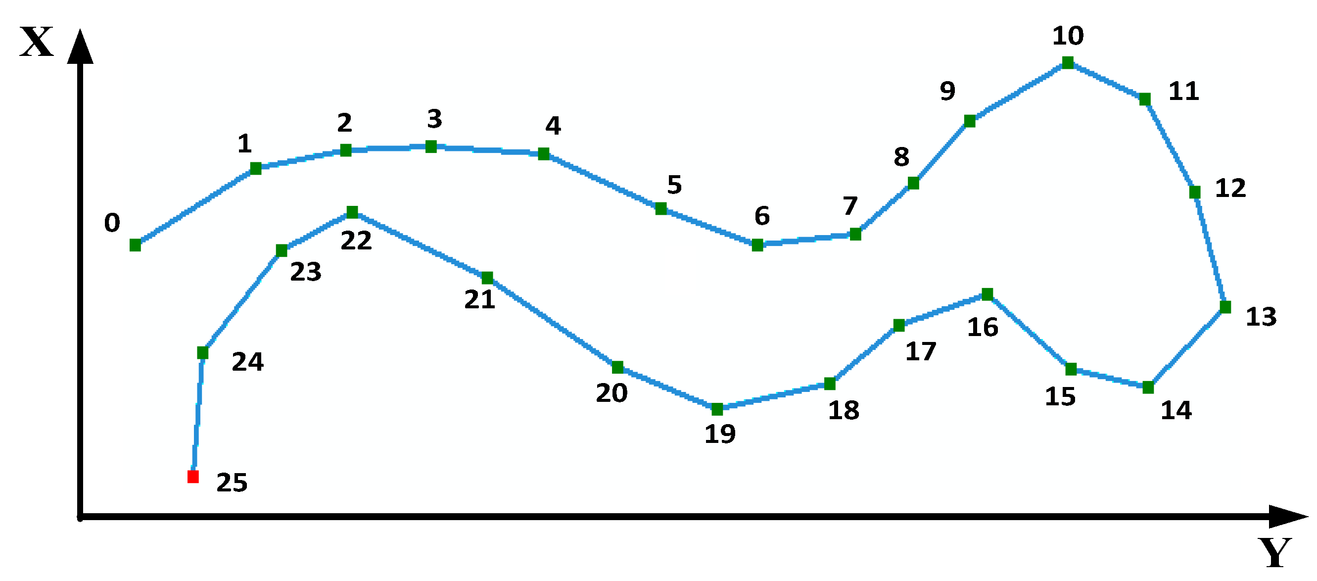
2.1. Basic Theory of the Douglas–Peucker (D–P) Algorithm

The D–P algorithm is a classic algorithm used for curve compression. The algorithm is used to simplify polylines by deleting non-feature vertices and retaining the feature vertices. The basic theory and computational steps of the D–P algorithm are as follows [1,24]:

Step 1: For a curve $L$, which is composed of $N$ coordinate vertices, the coordinate vertices set $V$ is written as $V=\left\{v_1,v_2,\dots ,v_i,\dots ,v_N\right\},\left(i=1,2,\dots ,N\right)$. First, connect the first vertex $v_1$ and the last vertex $v_N$, to obtain a new straight line $L_{v_1{v}_N}$. Second, calculate the shortest distances between the remaining vertices $\left\{v_2,\dots ,v_{N-1}\right\}$ and the new straight line $L_{v_1{v}_N}$ and obtain the shortest distance sets $D=\left\{D_2,\dots D_k,\dots ,D_{N-1}\right\}$ ($D_k$ is the shortest distance between vertex $v_k$ and the new straight line $L_{v_1{v}_N}$);

Step 2: Select the maximum distance ($D_{\max }$) with shortest distance $D$, $D_{\max }=D_k$ ($D_k$ is the shortest distance between vertex $v_k$ and the new straight line $L_{v_1{v}_N}$). Given a distance $\epsilon$ as the distance threshold, if $D_{\max }<\epsilon$, then the remaining vertices $\left\{v_2,\dots ,v_{N-1}\right\}$ from vertices set $V=\left\{v_1,v_2,\dots ,v_N\right\}$ are deleted, the given curve $L$ is compressed into a straight line $L_{v_1{v}_N}$ and the D–P algorithm is finished. If $D_{\max }\ge \epsilon$, then the vertices set $V=\left\{v_1,v_2,\dots ,v_N\right\}$ is divided into two subsets $V_t$ and $V_s$, that is, $V=V_t+V_s$ ($V_t=\left\{v_1,v_2,\dots ,v_k\right\}$, $V_s=\left\{v_k,v_{k+1},\dots ,v_N\right\}$);

Step 3: For the subsets $V_t$ and $V_s$, repeat step 1 and 2, respectively. If all of the calculated shortest distances are less than the giving distance threshold ($\epsilon$), then end the D–P algorithm.

2.2. Monotonic Chains and Dichotomy

The theory of the monotonic chain is mainly derived from computational geometry [12,25]. For the curve L, the monotonic chain is defined as follows:

Monotonic chain: For a curve $L$, which is composed of $M$ coordinate vertices, the coordinate vertices set $V$ is expressed as $V=\left\{v_1,v_2,\dots ,v_i,\dots ,v_M\right\},\left(i=1,2,\dots ,M\right)$; $x_i$ is the $X$-axis coordinate of vertex $v_i$, and $y_i$ is the $Y$-axis coordinate of vertex $v_i$. In the direction of the $X$-axis, for the coordinate vertices set $X=\left\{x_1,x_2,\dots ,x_i,\dots ,x_M\right\},\left(i=1,2,\dots ,M\right)$, if $x_i\le x_{i+1}$ $\left(i=1,2,\dots ,M\right)$ or $x_i>x_{i+1}$ $\left(i=1,2,\dots ,M\right)$, the curve $L$ will be called a monotonic increasing (or decreasing) chain of the X-axis. Similarly, in the direction of the $Y$-axis, for the coordinate vertices set $Y=\left\{y_1,y_2,\dots ,y_i,\dots ,y_M\right\},\left(i=1,2,\dots ,M\right)$ $\left(i=1,2,\dots ,M\right)$, if $y_i\le y_{i+1}$ $\left(i=1,2,\dots ,M\right)$ or $y_i>y_{i+1}$ $\left(i=1,2,\dots ,M\right)$, the curve $L$ will be called a monotonic increasing (or decreasing) chain of the Y-axis.

Dichotomy: Dichotomy is one of the most commonly used search algorithms for ordinal sequences and has a high search efficiency [12,13]. Given the target element $t$ and the ordered sequence $K=\left\{k_1,k_2,\dots ,k_i,\dots ,k_U\right\},\left(i=1,2,\dots ,U\right)$, ($t\in K$), to search for the target element $t$ from $K$, the basic theory of dichotomy is as follows:

Step 1: For the target element $t$, compare $t$ with the intermediate element $k_{\frac{U}{2}}$ from the sequence $K$. If $t\ne k_{\frac{U}{2}}$, then $K$ will be divided into two parts: $K_1$ and $K_2$, $K=K_1\cup K_2$, $K_1=\left\{k_1,k_2,\dots ,k_i,\dots ,k_{\frac{U}{2}}\right\}$ $\left(i=1,2,\dots ,U\right)$, $K_2=\left\{k_{\frac{U}{2}},k_{\frac{U}{2}+1},\dots ,k_j,\dots ,k_U\right\}$ $\left(j=\frac{U}{2},\frac{U}{2}+1,\dots ,U\right)$.

Step 2: For the target element $t$, if $t\ge k_{\frac{U}{2}}$, then execute step 1 in the $K_2$ until the target element $t$ is found from the ordered $K_2$; if $t<k_{\frac{U}{2}}$, then execute step 1 in the $K_1$ until the target element $t$ is found from the ordered $K_1$.

In vector spatial data structure, it is well known that a simple curve is composed of a number of line segments. For a curve $L$, there are $N$ coordinate vertices: $P=\left\{p_1,p_2,\dots ,p_i,\dots ,p_N\right\},\left(i=1,2,\dots ,N\right)$, and the curve $L$ is composed of some line segments, such as: $L=L_{1,2}^{\prime }+L_{2,3}^{\prime }+\dots +L_{i,j}^{\prime }+\dots +L_{N-1,N}^{\prime }$ ($N$ is the number of the coordinate vertices). Figure 2, shows that curve $L$ is composed of 26 coordinate vertices ($0,1,2,\dots ,25$). In the Gauss-Krueger plane rectangular coordinate system, the horizontal axis was the Y-axis, and the vertical axis was the X-axis. Along the Y-axis, $L$ could be divided into two monotonic chains $L_i^{\prime }$ ($i=0,1,2,\dots ,13$) and ${L^{\prime }}_j{}_i$ ($j=13,14,\dots ,25$). For ${L^{\prime }}_i$, along the $Y$-axis, vertex $p_0$ is the smallest, and the vertex $p_{13}$ is the biggest, and ${L^{\prime }}_i$ is a monotonic increasing chain; For ${L^{\prime }}_j$, along the $Y$-axis, vertex $p_{13}$ is the biggest, and the vertex $p_{25}$ is the smallest, and ${L^{\prime }}_j$ is a monotonic decreasing chain. When using the D–P algorithm to process the curve $L$, it should be noted that if the final result has self-intersection problems, it has been caused by the corresponding monotonic chains ${L^{\prime }}_i$ and ${L^{\prime }}_j$.

2.3. The New Vector Line Simplification Algorithm based on the D–P Algorithm, Monotonic Chains and Dichotomy

This paper used the monotonic chains and dichotomy to solve the self-intersection problem in spatial line simplification when processed by the D–P algorithm. In our proposed method, we firstly use the D–P algorithm to simplify the original polyline $M$, and obtain the simplified polyline $T$; Secondly, we check the self-intersection problems of $T$. If $T$ does not have self-intersection problems, then we end this proposed method, otherwise, we use monotonic chain technology to quickly divide the $T$ into several sequential monotonic chains; Thirdly, the dichotomy, MER (minimum-area enclosing rectangle, which refers to the rectangle with the smallest area that encloses the polyline) and geometric calculation method are used to process the sequential monotonic chains, in order to quickly locate the positions of the self-intersection problems of the sequential monotonic chains and solve the self-intersection problems, to obtain the final results.

This strategy of the proposed method does not only take the curve characteristics of a polyline into account, but also improves the time consumption of the proposed method. The main steps of the proposed method are described below.

Step 1: Use the D–P algorithm to process one curve $M$ (There aren’t self-intersection errors of $M$) and obtain a new curve $T$.

Step 2: Check the self-intersection problems of the $T$; if there are self-intersection errors, then perform step 3; otherwise, $T$ is the final result of line simplification.

Step 3: For $T$, after step 2 of processing, if there are self-intersection errors, according to the sequence of the coordinate vertices, use the monotonic chain technology (as described in Section 2.2) to divide $T$ into several sequential monotonic chains $T_1{}^{\prime }$, $T_2{}^{\prime }$, …, $T_i{}^{\prime }$, …, $T_j{}^{\prime }$, …, $T_n{}^{\prime }$ $\left(i,j\in [1,n]\right)$.

Step 4: For monotonic chains $T_i{}^{\prime }$ and $T_j{}^{\prime }$, which include and coordinate vertices, respectively, if $n\ge m$, then use the dichotomy to quickly divide $T_i{}^{\prime }$ into two monotonic chains: ${L^{\prime }}_{1,t}$ and ${L^{\prime }}_{t,n}$ ($t=\frac{n}{2}$, when $n$ was even; or $t=\frac{n}{2}+1$, when $n$ was odd, $n$ is an integer, and $n>1$), ${L^{\prime }}_{1,t}$ and ${L^{\prime }}_{t,n}$ are also two monotonic chains. Similarly, if $n<m$, then divide $T_j{}^{\prime }$ into two monotonic chains ${S^{\prime }}_{1,t}$ and $S_{t,m}^{\prime }$ ($t=\frac{m}{2}$, when $m$ was even; or $t=\frac{m}{2}+1$, when $m$ was odd, $m$ is an integer, and $m>1$), ${S^{\prime }}_{1,t}$ and $S_{t,m}^{\prime }$ are also two monotonic chains.

Step 5: If $n\ge m$, calculate the MER of ${L^{\prime }}_{1,t}$, ${L^{\prime }}_{t,n}$ and ${T^{\prime }}_j$, respectively, as $R_{L_{1,t}}$, $R_{L_{t,n}}$ and $R_{T_j}$. Similarly, if $n<m$, calculate the MER of ${S^{\prime }}_{1,t}$, $S_{t,m}^{\prime }$ and ${T^{\prime }}_i$, respectively, as $R_{S_{1,t}}$, $R_{S_{t,n}}$ and $R_{T_i}$.

Step 6: For $R_{L_{1,t}}$, $R_{L_{t,n}}$ and $R_{T_j}$, if $R_{L_{1,t}}\cap R_{T_j}$ = $R_{L_{t,n}}\cap R_{T_j}$ = $\varphi$, then there is a non-intersection between $T_i{}^{\prime }$ and $T_j{}^{\prime }$; If $R_{L_{1,t}}\cap R_{T_j}$ $\ne \varphi$, and $R_{L_{t,n}}\cap R_{T_j}=\varphi$, then there may be an intersection problem between the monotonic chain ${L^{\prime }}_{1,t}$ and $T_j{}^{\prime }$, and there is a non-intersection between ${L^{\prime }}_{t,n}$ and $T_j{}^{\prime }$; If $R_{L_{1,t}}\cap R_{T_j}$ = $\varphi$, and $R_{L_{t,n}}\cap R_{T_j}$ $\ne \varphi$, there may be an intersection problem between the monotonic chain ${L^{\prime }}_{t,n}$ and $T_j{}^{\prime }$, and there is a non-intersection between ${L^{\prime }}_{1,t}$ and $T_j{}^{\prime }$; If $R_{L_{1,t}}\cap R_{T_j}$ $\ne \varphi$, and $R_{L_{t,n}}\cap R_{T_j}$ $\ne \varphi$, then there may be an intersection problem between the monotonic chain ${L^{\prime }}_{1,t}$ and $T_j{}^{\prime }$, and there may be an intersection problem between the monotonic chain ${L^{\prime }}_{t,n}$ and $T_j{}^{\prime }$. Using the same method, we can calculate whether there are intersection problems between $R_{S_{1,t}}$, $R_{S_{t,n}}$, and $R_{T_i}$.

Step 7: Process all of the sequential monotonic chains $T_1{}^{\prime }$, $T_2{}^{\prime }$, …, $T_i{}^{\prime }$, …, $T_j{}^{\prime }$, …, $T_n{}^{\prime }$ $\left(i,j\in [1,n]\right)$ using step 4, step 5, and step 6, until all the intersection problems of the monotonic chains are found.

Step 8: After processing by step 1 to step 7, all the intersection problems of the monotonic chains are found. In this step, we take an example to show how the proposed method deals with these intersection problems.

For one curve $T$, which is processed by the D–P algorithm as shown in Figure 3a, $T$ includes 25 coordinate vertices. Using step 2 and step 3, we can obtain three monotonic chains $T_1{}^{\prime }$, $T_2{}^{\prime }$ and $T_3{}^{\prime }$ (as shown in Figure 3b); $T_1{}^{\prime }$ contains six coordinate vertices ($P_1,\dots ,P_6$), and $P_1$ and $P_6$ are the end vertices of $T_1{}^{\prime }$; $T_2{}^{\prime }$ contains nine coordinate vertices ($P_6,\dots ,P_{14}$), and $P_6$ and $P_{14}$ are the end vertices of $T_2{}^{\prime }$; $T_3{}^{\prime }$ contains 12 coordinate vertices ($P_{14},\dots ,P_{25}$), and $P_{14}$ and $P_{25}$ are the end vertices of $T_3{}^{\prime }$. After using step 4, step 5, step 6 and step 7, there is one intersection problem between $T_1{}^{\prime }$ and $T_3{}^{\prime }$, and there is another intersection problem between $T_2{}^{\prime }$ and $T_3{}^{\prime }$.

Using Figure 3c as an example, after processing by step 6, assuming that there is one intersection problem between $T_1{}^{\prime }$ and $T_3{}^{\prime }$, to obtain the intersection line segment $K_{5,6}$ and $K_{17,18}$ by the geometric calculation method [12,25] and obtain the coordinate vertices $P_5$, $P_6$, and $P_{17}$, $P_{18}$. If there are coordinate vertices $\left(v_p,v_{p+1},\dots v_i,\dots ,v_q,i\in [p,q]\right)$ ($p,q$ are two integers) between $P_{17}$ and $P_{18}$ that belong to the original curve $M$, then calculate the shortest distance between the vertices $\left(v_p,v_{p+1},\dots v_i,\dots ,v_q,i\in [p,q]\right)$ and the line segment $K_{17,18}$ and find the maximum value ($D_{\max }$) of the shortest distance and the corresponding coordinated point $P_i$.

Connect $P_{17}{P}_i$, and $P_i{P}_{18}$ and obtain two new monotonic chains $T_{17i}{}^{\prime }$ and $T_{i18}{}^{\prime }$. Calculate whether there are intersection problems between the two new monotonic chains $T_{17i}{}^{\prime }$, $T_{i18}{}^{\prime }$ and the monotonic chain $T_1{}^{\prime }$. If there are no intersection problems, then conclude this algorithm; the monotonic chain $T_3{}^{\prime }$ will be divided into two new monotonic chains $T_{17i}{}^{\prime }$ and $T_{i18}{}^{\prime }$. If there are other intersection errors, then re-execute step 8 and step 9 until there is no intersection error between $T_1{}^{\prime }$ and $T_3{}^{\prime }$.

Similarly, if there are coordinate vertices between $P_5$ and $P_6$ that belong to the original curve $M$, re-execute steps 8 and 9 until there is no intersection error between $T_1{}^{\prime }$ and $T_3{}^{\prime }$.

Execute steps 4 to 8 until there are no intersection errors between all the monotonic chains, and then obtain the final result $T^{\prime }$. Figure 3d shows the final result, $k_i$ and $k_j$ are two coordinate vertices from the original curve $M$.

Step 9: After processed by step 1 to step 8, all of the intersection problems have been processed, then end the proposed method, and obtain the final results.

3. Experiments and Analysis

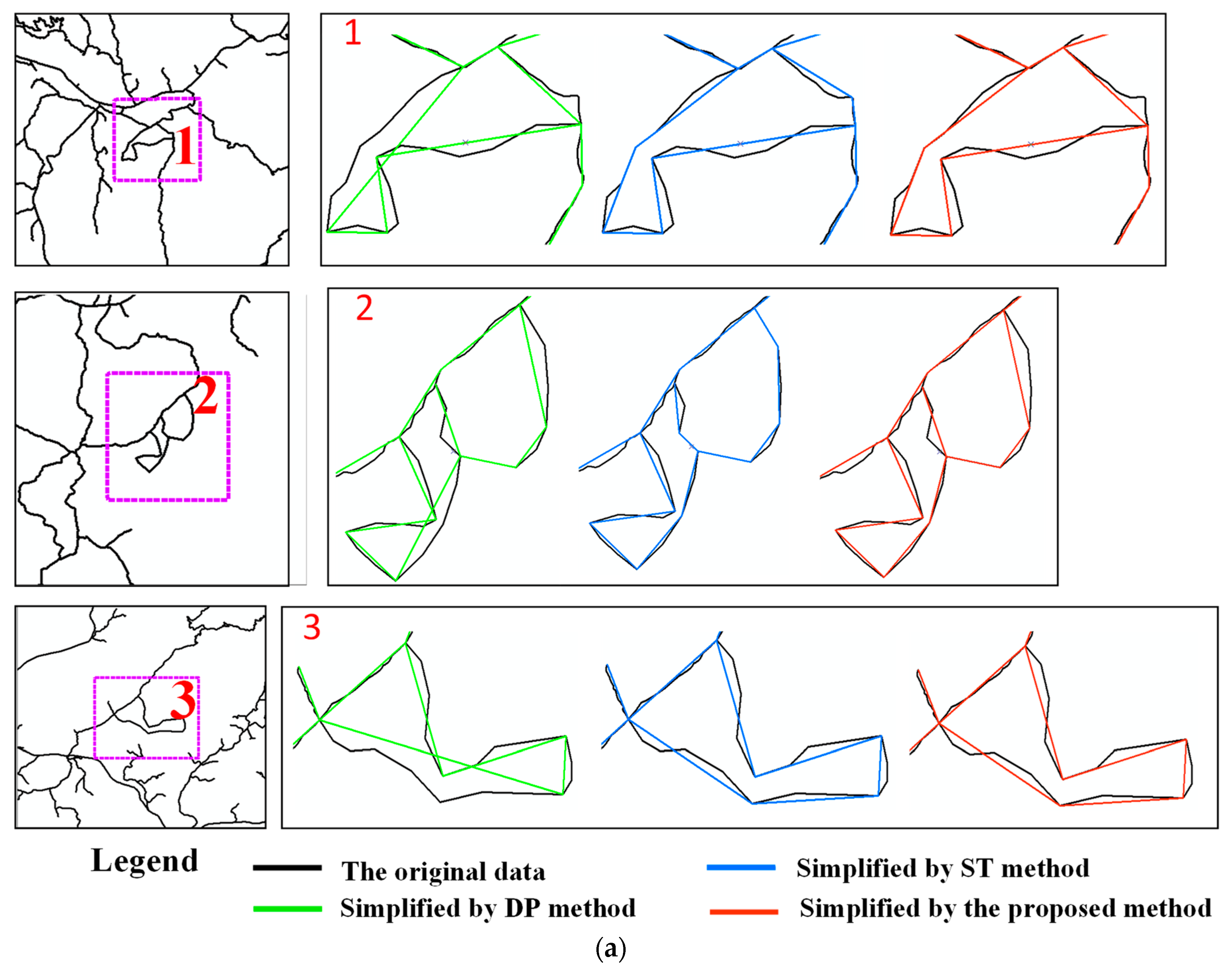
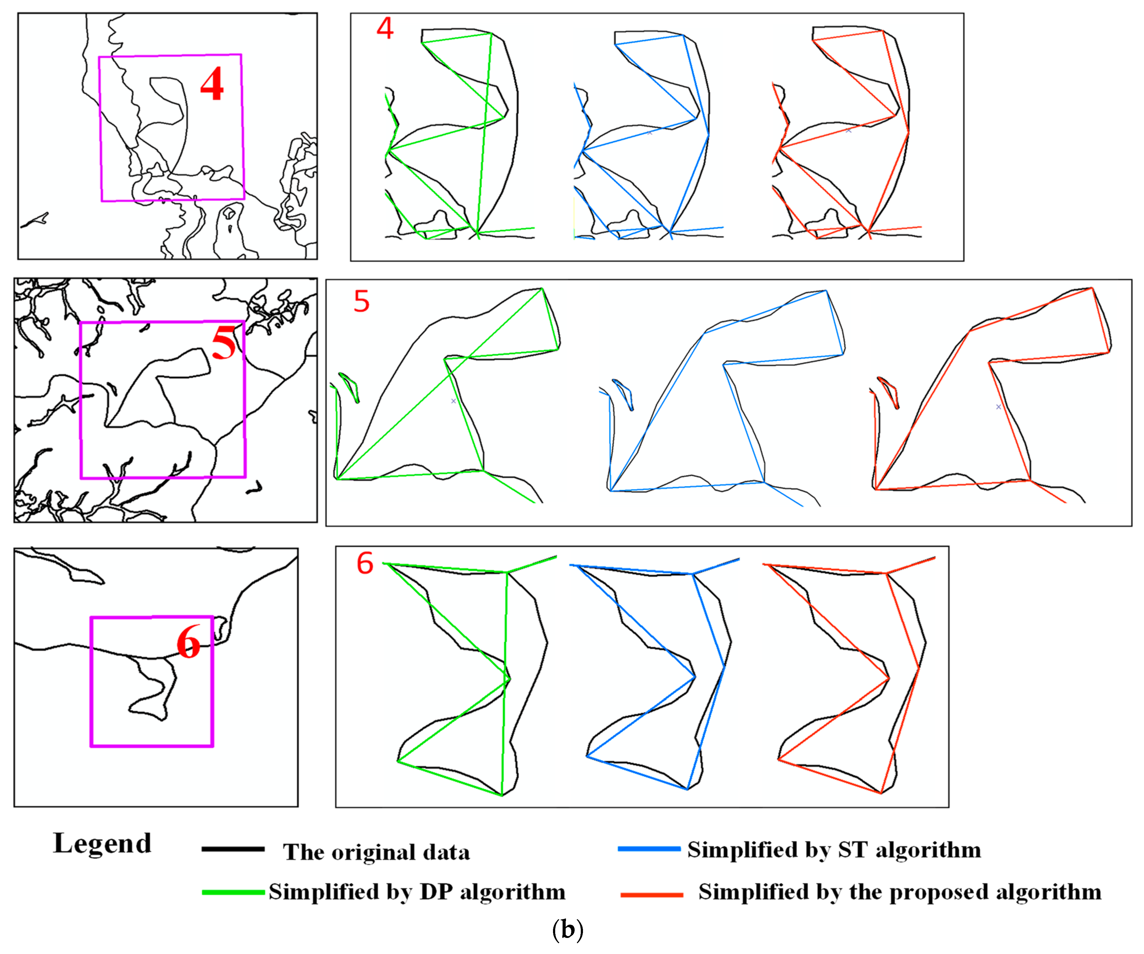
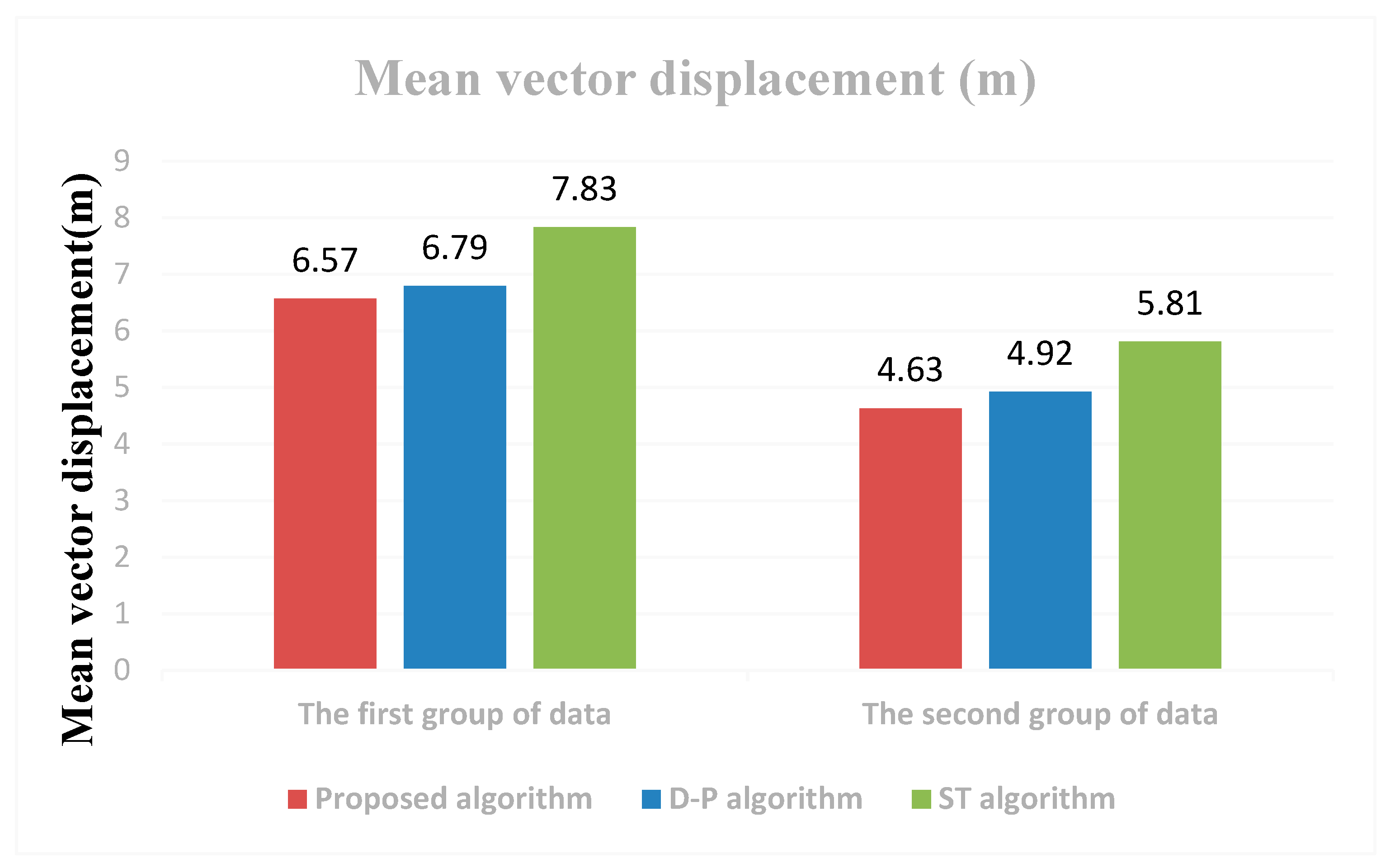
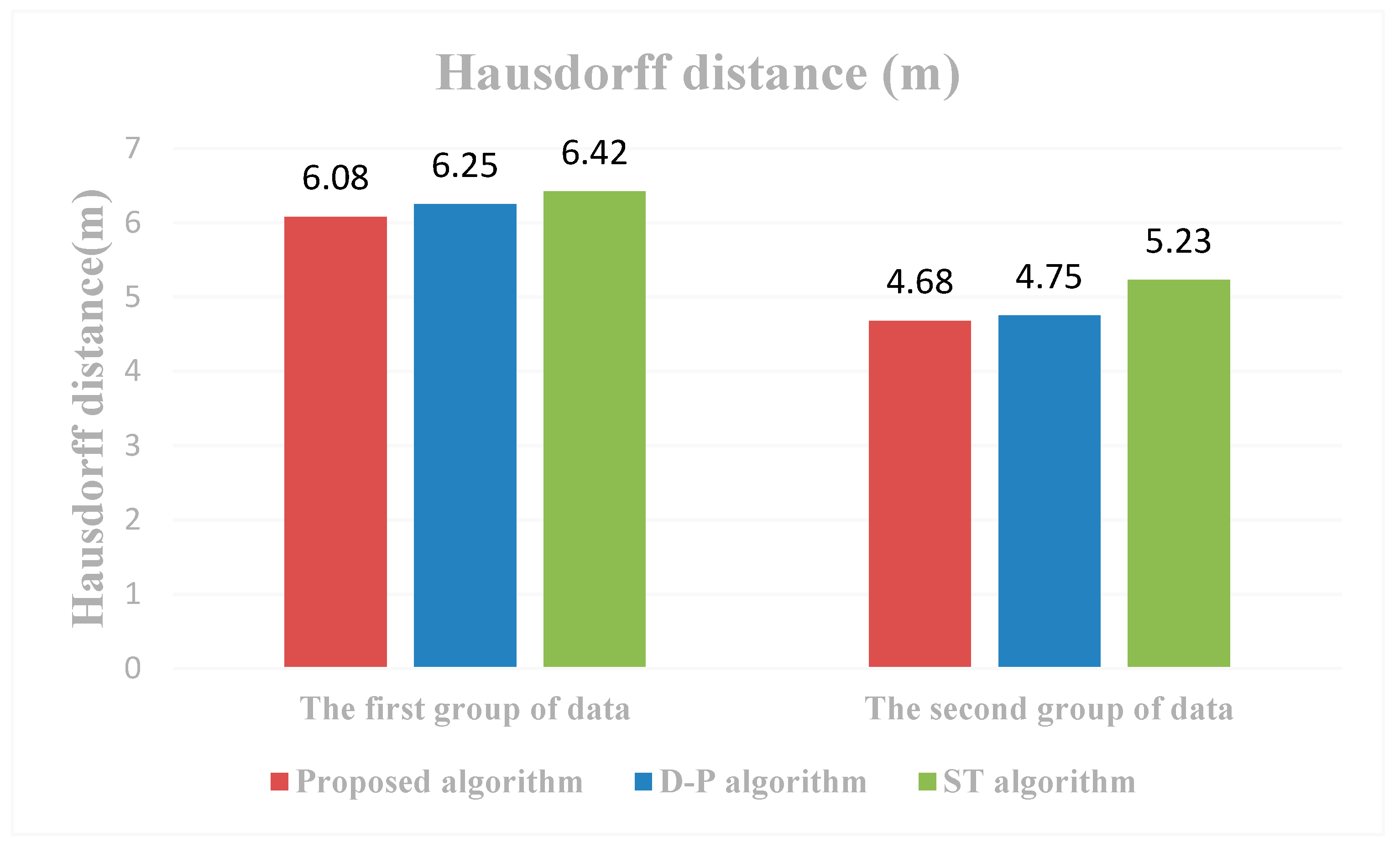
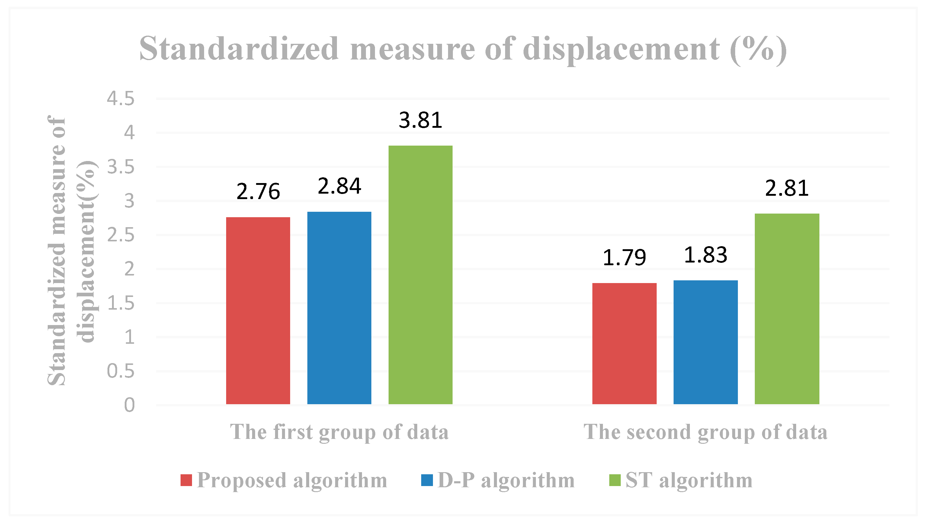
We select two groups of experimental data to verify the validity of the proposed algorithm. The first group of data is the road line of Jiangxi Province in China. Its total length is approximately 1.56 × 10⁵ km, and the data volume is approximately 92,000 bytes, including approximately 5.13 × 10⁶ vertices. The second group of data is the land use line of Dingnan County in Jiangxi Province in China. Its total length is approximately 1.41 × 10⁴ km, and the data volume is approximately 26,000 bytes, including approximately 1.24 × 10⁶ vertices.

3.1. Assessment

In this study, we adopted a number of different methods to simplify the two groups of data and compare the performance of the proposed method. This is due to the ST algorithm [23], which is also based on the D–P algorithm, which could solve the self-intersection problems, in this paper, we compared the performance of the proposed method with the ST algorithm and the D–P algorithm.The scale of the experimental data is 1:10,000, and the results in target proportions of the original vertices are 60% and 70%, respectively. As a result, the two groups of the data are displayed as large volumes. Thus it is difficult to show case further details, in the same experimental environment. Moreover, we chose six self-intersection problems from the two groups of data instead. The simplified results of the six self-intersection problems are shown in Figure 4.

As is shown in Figure 4, the simplified results brought up from each group of data, the D–P algorithm produced self-intersection problems, but the proposed method could process self-intersection problems as well as the ST algorithm. To compare the performance of the different methods, four metrics are selected, including time consumption, mean vector displacement [3,26], Hausdorff distance (HD) [27], and standardized measure of displacement (SMD) [28].

Time consumption indicates how much time the algorithm takes.

Mean vector displacement is computed as the average displacement of the vector between the original vertices and the simplified version of the same vertices.

The Hausdorff distance (HD) between the two geometric objects is the largest minimum distance between points on one object to the other [27].

Standardized measure of displacement (SMD) is defined by Joao [28], and the calculation formula is demonstrated as follows:

$$SMD(\%)=(1-(W-O)/W)\times 100$$

(1)

$W$ is the distance from the coordinate vertices which has the maximum displacement between the original polyline and the simplified polyline to the straight line. This is obtained by connecting the first and last nodes of the polyline, and $O$ is the actual displacement of the coordinate vertices between the original polyline and the simplified polyline.

3.2. Results

The simplification assessment metrics of the data processed data by method are shown as follows: the resulting statistics are computed using the two groups of experimental datasets.

(1) Time consumption: the time consumption results of the three line simplification methods are shown in Figure 5, and the time consumption is measured in milliseconds (ms).

(2) Mean vector displacement: the mean vector displacement results of the three line simplification methods are shown in Figure 6. The mean vector displacement is measured in meters (m).

(3) Hausdorff distance (HD): the Hausdorff distance (HD) results of the three line simplification methods are shown in Figure 7. The HD is measured in meters (m).

(4) Standardized measure of displacement (SMD): the standardized measure of displacement (SMD) results of the three line simplification methods are shown in Figure 8.

3.3. Analysis

From Figure 5 to Figure 8, we observe the following:

(1) The proposed method can be used effectively for vector line simplification. We used two groups of data to verify the proposed method. It can be shown from the experimental results that the proposed method can not only solve the problem of self-intersection caused by the D–P algorithm but also has a high execution efficiency. Figure 4 shows the six results of simplifying the two groups of data using the three methods. In the six self-intersection problems as shown in the Figure 4, the polylines of six regions demonstrate complex curves with a number of hierarchical bends. As shown in Figure 4, the D–P algorithm produces self-intersection problems, but the proposed method and ST algorithm avoid these problems. This is due to the ST algorithm also being based on the D–P algorithm. As a result, the three methods identified the same experimental results in some cases.

(2) The D–P algorithm was found to have $O\left(nm\right)$ the worse case time and $O\left(n\log n\right)$ expected time, where $n$ was the number of input vertices and $m$ was the number of simplified polyline segments [23]; The ST algorithm was composed of mainly three steps; the worst case $O\left(nm\right)$ time complexity, where $n$ was the number of input vertices and $m$ depended on the number of star-shaped regions [23]. The proposed method in this paper involved two key steps: first, we first used the D–P algorithm to simplify the original curves and checked the self-intersection problems; then, we used the monotonic chain and dichotomy methods to address the self-intersection values. In the first step, our algorithm had the same execution time as the D–P algorithm. In the second step, our algorithm was carried out in $O\left(m\log m\right)$ time, while $m$ was the number of self-intersection segments of simplified polylines.

The time consumption results of the three methods for processing the two groups of data are shown in Figure 5. For the first group of data, the time consumption results of the D–P algorithm, the proposed method and ST algorithm are 5,523,375 ms, 6,954,155 ms, and 10,283,326 ms, respectively. For the second group of data, the time consumption results of the D–P algorithm, the proposed method and ST algorithm are 75,325 ms, 93,256 ms, and 310,201 ms, respectively. It can be seen from the experimental results of each group of data that the time consumption of the proposed method is slightly higher than the D–P algorithm with the proposed method and, after the procession of the D–P algorithm, we use monotonic chains and dichotomy to modify the self-intersection problems. It is obvious that the time consumption of the proposed method is much lower than the ST algorithm. This is because the monotonic chains and dichotomy have high search efficiency and can quickly find and solve the self-intersection problems that are processed by the D–P algorithm.

(3) We use mean vector displacement to measure the location accuracy. As shown in Figure 6, the first group of data, the mean vector displacement results of the D–P algorithm, the proposed method and ST algorithm are 6.79 m, 6.57 m, and 7.83 m, respectively, The second group of data showed that the mean vector displacement results of the D–P algorithm, the proposed method and ST algorithm are 4.92 m, 4.63 m, and 5.81 m, respectively. For each group of data, the mean vector displacement of the proposed method is similar to the D–P algorithm but much lower than the ST algorithm.

(4) Figure 7 shows the Hausdorff distance of the three methods for processing the two groups of data. For the first group of data, the Hausdorff distances of the D–P algorithm, the proposed method and ST algorithm are 6.25 m, 6.08 m, and 6.85, respectively. The second group of data showed, the Hausdorff distances of the D–P algorithm, the proposed method and ST algorithm are 4.75 m, 4.68 m, and 5.23 m, respectively. For each group of the data, the Hausdorff distance of the proposed method is similar to the D–P algorithm and the ST algorithm.

(5) We also used a standardized measure of displacement (SMD) to measure the location accuracy. As shown in Figure 8, the first group of data, the SMDs of the D–P algorithm, the proposed method, and ST algorithm are 3.46%, 3.58%, and 4.25%, respectively, The second group of data showed that the SMDs of the D–P algorithm, the proposed method and ST algorithm are 1.83%, 1.79%, and 2.81%, respectively. For each group of data, the mean vector displacement of the proposed method is similar to the D–P algorithm but much lower than the ST algorithm.

4. Conclusions

Vector line simplification is widely used in computer graphics, GIS, and others. The D–P algorithm is one of the most widely used methods for vector line simplification. When professionals use the D–P algorithm to address complex curves, we find it is easy to produce self-intersection problems. To further expand the application of the D–P algorithm, in this paper a new line simplification algorithm that combines the D–P algorithm, monotonic chains, and dichotomy is proposed. In the end, two experiments are designed to compare the results of our proposed method with the D–P algorithm and ST algorithm. From the result analysis, it is clear that the proposed algorithm has several advantages: (1) compared with the D–P algorithm, the proposed algorithm has the same execution efficiency but without self-intersection problems; (2) compared with the ST algorithm, the proposed method has the same ability to solve self-intersection problems but has better execution efficiency. At the same time, the proposed algorithm also has shortcomings to be further studied: (1) the proposed method focuses on the removal of self-intersection problems, however, the area preservation problems after the polyline simplification are not considered; (2) similar to the D–P algorithm, this proposed method does not consider the bending characteristics of the curves. In conclusion, these two thematic shortcomings will be the focus of our future research.

References

1. Douglas, D.H.; Peucker, T.K. Algorithms for the reduction of the number of points required to represent a digitized line or its caricature. Can. Cartogr. 1973, 10, 112–122. [Google Scholar] [CrossRef] [Green Version]
2. Ramer, U. An iterative procedure for the polygonal approximation of plane curves. Comput. Graph. Image Process. 1972, 1, 244–256. [Google Scholar] [CrossRef]
3. Lang, T. Rules for robot draughtsmen. Geogr. Mag. 1969, 42, 50–51. [Google Scholar]
4. McMaster, R.B. The integration of simplification and smoothing algorithms in line generalization. Can. Cartogr. 1989, 26, 101–121. [Google Scholar] [CrossRef]
5. Li, Z.L. An Algorithm for Compressing Digital Contour Data. Cartogr. J. 1988, 25, 143–146. [Google Scholar] [CrossRef]
6. Visvalingam, M.; Whyatt, J. Line generalisation by repeated elimination of the smallest area. Technical Report, Discussion Paper 10, Cartographic Information Systems Research Group (CISRG); The University of Hull: Hull, UK, 1992. [Google Scholar]
7. Ratschek, H.; Rokne, J.; Leriger, M. Robustness in GIS algorithm implementation with application to line simplification. Int. J. Geogr. Inf. Sci. 2001, 15, 707–720. [Google Scholar] [CrossRef]
8. Wang, Z.S.; Muller, J.-C. Line Generalization Based on Analysis of Shape Characteristics. Cartogr. Geogr. Inf. Syst. 1998, 25, 3–15. [Google Scholar] [CrossRef]
9. Zhao, Z.; Saalfeld, A. Linear-Time Sleeve-Fitting Polyline simplification algorithms. In Proceedings of the AutoCarto 13, Seattle, WA, USA, 7–10 April 1997; Published by American Congress on Surveying and Mapping & American Society for Photogrammetry and Remote Sensing, Maryland. pp. 214–223, ISBN -1-57083-043-6. [Google Scholar]
10. Gary, R.H.; Wilson, A.D.; Archuleta, C.M.; Thompson, F.E.; Vrabel, J. Production of a National 1:1000000-Scale Hydrography Dataset for the United States: Feature selection, Simplification, and Refinement; U.S. Geological Survey Scientific Investigations Report 2009–5202. Revised May 2010; U.S. Geological Survey: Reston, VA, USA, 2010; 22p. [CrossRef]
11. Li, Z.L.; Openshaw, S. Algorithms for automated line generalization based on a natural principle of objective generalization. Int. J. Geogr. Inf. Sci. 1992, 6, 373–389. [Google Scholar] [CrossRef]
12. Samsonov Timofey, E.; Yakimova, O.P. Shape adaptive geometric simplification of heterogeneous line datasets. Int. J. Geogr. Inf. Sci. 2017, 31, 1485–1520. [Google Scholar] [CrossRef]
13. de Berg, M.; van Kreveld, M.; Overmars, M.; Overmars, M.; Schwarzkopf, O. Computational Geometry: Algorithms and Applications, 2nd ed.; Springer: Berlin, Germany, 2000. [Google Scholar]
14. Cromley, R.G. Principal axis line simplification. Comput. Geosci. 1992, 18, 1003–1011. [Google Scholar] [CrossRef]
15. Raposo, P. Scale-specific automated line simplification by vertex clustering on a hexagonal tessellation. Cartogr. Geogr. Inf. Syst. 2013, 40, 427–443. [Google Scholar] [CrossRef]
16. Kronenfeld, B.J.; Stanislawski, L.V.; Buttenfield, B.P.; Tyler, B. Simplification of polylines by segment collapse: Minimizing areal displacement while preserving area. Int. J. Cartogr. 2020, 6, 22–46. [Google Scholar] [CrossRef]
17. Shi, W.Z.; Cheung, C.K. Performance Evaluation of Line Simplification Algorithms for Vector Generalization. Cartogr. J. 2006, 43, 27–44. [Google Scholar] [CrossRef]
18. Mi, X.J.; Sheng, G.M.; Zhang, J.; Bai, H.X.; Hou, W. A new algorithm of vector date compression based on the tolerance of area error in GIS. Sci. Geogr. Sin. 2012, 32, 1236–1240. [Google Scholar]
19. Saalfeld, A. Topologically consistent line simplification with the Douglas-Peucker algorithm. Cartogr. Geogr. Inf. Sci. 1999, 26, 7–18. [Google Scholar] [CrossRef]
20. Ho, P.S.; Kim, M.H. A hierarchical scheme for representing curves without self-intersections. In Proceedings of the 2001 IEEE Computer Society Conference (CVPR 2001), Kauai, HI, USA, 8–14 December 2001. [Google Scholar] [CrossRef]
21. Mantler, A.; Snoeyink, J. Safe sets for line simplification. In 10th Annual Fall workshop on Computational Geometry; Stony Brok University: New York, NY, USA, 2000; Available online: http://citeseerx.ist.psu.edu/viewdoc/summary?doi.10.1.1.32.402 (accessed on 29 March 2020).
22. Avelar, S.; Müller, M. Generating topologically correct schematic maps. In Proceedings of the 9th International Symposium on Spatial Data Handling; Technical Report; Swiss Federal Institute of Technolog Zurich: Zurich, Switzerland, 2000; pp. 4–28. [Google Scholar] [CrossRef]
23. Wu, S.T.; Marquez, M.R.G. A non-self-intersection Douglas-Peucker algorithm. In Proceedings of the 16th Brazilian Symosium on Computer Graphics and Image Processing (SIBGRAPI), Sao Carlos, Brazil, 12–15 October 2003. [Google Scholar] [CrossRef] [Green Version]
24. Ebisch, K. Short note: A correction to the Douglas-Peucker line generalization. Comput. Geosci. 2002, 28, 995–997. [Google Scholar] [CrossRef]
25. Yan, H.W.; Wang, M.X.; Wang, Z.H. Computational Geometry: Spatial Data Processing Algorithm; Science Press: Beijing, China, 2012. [Google Scholar]
26. White, E.R. Assessment of line-generalization algorithms using characteristic points. Cartogr. Geogr. Inf. Sci. 1985, 12, 17–28. [Google Scholar] [CrossRef]
27. Hangouët, J.F. Computation of the Hausdorff distance between plane vector polylines. In Auto-Carto XII: Proceedings of the International Symposium on Computer-Assisted Cartography, Charlotte, North Carolina; American Congress on Surveying and Mapping & American Society for Photogrammetry and Remote Sensing: Gaithersburg, MD, USA, 1995; Volume 4, pp. 1–10. ISBN -1-57083-019-3. [Google Scholar]
28. Joao, E.M. Gauses and Consequences of Map Generalization; Taylor and Francis: London, UK, 1998. [Google Scholar]
Figure 1. The flowchart of the proposed method.
Ijgi 09 00251 g001
Figure 2. A schematic chart of the monotonic chain.
Ijgi 09 00251 g002
Figure 3. (a) The curve T which processed by D–P algorithm; (b) three monotonic chains T 1 , T 2 and T 3 processed by the monotonic chain technology; (c) minimum-area enclosing rectangle (MER) of T 1 and T 3 ; (d) the final result T .
Ijgi 09 00251 g003
Figure 4. The six simplified results of the three applied methods from the two groups of data. (a) The three self-intersection problems identified from the first group of data; (b) the three self-intersection problems identified from the second group of data. Notes: DP algorithm is the Douglas–Peucker algorithm proposed by Douglas and Peucker [1]; ST algorithm is the star-shaped algorithm proposed by Wu and Marquez [23].
Ijgi 09 00251 g004aIjgi 09 00251 g004b
Figure 5. Time-consumption results. (a) Time consumption of the first group of data; (b) time consumption of the second group of data.
Ijgi 09 00251 g005
Figure 6. The mean vector displacement results (m).
Ijgi 09 00251 g006
Figure 7. The Hausdorff distance results (m).
Ijgi 09 00251 g007
Figure 8. The standardized measure of displacement results (%).
Ijgi 09 00251 g008