A New Architecture of Densely Connected Convolutional Networks for Pan-Sharpening

Abstract

In this paper, we propose a new architecture of densely connected convolutional networks for pan-sharpening (DCCNP). Since the traditional convolution neural network (CNN) has difficulty handling the lack of a training sample set in the field of remote sensing image fusion, it easily leads to overfitting and the vanishing gradient problem. Therefore, we employed an effective two-dense-block architecture to solve these problems. Meanwhile, to reduce the network architecture complexity, the batch normalization (BN) layer was removed in the design architecture of DenseNet. A new architecture of DenseNet for pan-sharpening, called DCCNP, is proposed, which uses a bottleneck layer and compression factors to narrow the network and reduce the network parameters, effectively suppressing overfitting. The experimental results show that the proposed method can yield a higher performance compared with other state-of-the-art pan-sharpening methods. The proposed method not only improves the spatial resolution of multi-spectral images, but also maintains the spectral information well.

1. Introduction

In recent years, remote sensing image analysis has attracted much attention. Greatly successful applications have been achieved in the fields of hyperspectral (HSI) classification [1], anomaly detection [2], HSI unmixing [3], super-resolution [4], pan-sharpening, and so on. Due to the physical limitations of a single remote sensing imaging device, there is a tradeoff between the spatial and spectral resolution in the remote sensing images [5]. Therefore, the remote sensing satellites always carry panchromatic sensors and multispectral sensors to simultaneously benefit from both spatial and spectral information, such as QuickBird, IKONOS, and World-view. Multispectral sensors collect multidimensional information, such as spectral and polarization characteristics, while collecting two-dimensional spatial information to obtain multispectral (MS) images with a rich spectrum. However, the spatial resolution of the MS images is low. The panchromatic sensors capture high spatial resolution panchromatic (PAN) image with one channel, which is very disadvantageous for the recognition and determination of terrain types [6,7,8]. Pan-sharpening aims to combine the spatial features of PAN images and the spectral features of MS images into a fused image [9]. The fused image would not only have high spatial resolution, but also a rich spectrum to achieve the purpose of image enhancement.

To obtain more comprehensive and accurate scene descriptions, pan-sharpening applied as a post-processing technique can overcome the limitations of single sensor images, improve image clarity and understandability, and facilitate further image analysis and processing. Currently, the common pan-sharpening methods mainly include spatial domain methods, transformation domain methods, compressed sensing-based methods, and machine learning-based methods.

Spatial domain methods primarily use simple arithmetic or substitution algorithms to process image pixels directly and include the Brovey method [10], the intensity-hue-saturation (IHS) methods [11,12], and the principal component analysis (PCA) method [13]. The Brovey transformation method achieves fusion by preserving the spectral features of each pixel and multiplying the high-resolution PAN image and the proportion of each band of the low-resolution MS images. The IHS transformation is used to transform the low-resolution MS images from the RGB to the IHS color space. Then, the I component is replaced by the high-resolution PAN image after histogram matching, and the pan-sharpened MS images are obtained by the IHS inversion transformation. PCA is mainly aimed at low-resolution MS images, which are represented by three principal components. These principal components are independent. In the process of image fusion, the first principal component is fused because it includes the main information of MS images. The PRACSalgorithm employs the partial replacement of the intensity component, instead of using the PAN image directly, and proposes a new method to compute the benefit [14]. This kind of method has the characteristics of high efficiency and ease of implementation, but it will cause serious spectral distortion.

The transform domain algorithm first transforms the original image, then fuses the transform coefficients of the transform domain to obtain the transform coefficients of the fusion image, and finally, reconstructs the fusion image by inverse transformation. Common pan-sharpening algorithms based on the transform domain mainly include pyramid transform [15], wavelet transform [16,17], and multiscale geometric transform [18,19]. Wavelet transform technology has been widely used in pan-sharpening processing, which has effectively solved the problem of generating many redundant data based on the pyramid transform method. Although wavelet transform can decompose the image into multiple scales and multiple direction, the decomposition coefficients of the horizontal, vertical, and diagonal directions can be obtained, which are not conducive to the detailed description of the image. In order to overcome the shortcomings of wavelet transform, a new optimal representation method of high-dimensional function multi-scale geometric transform came into being. Common multiscale geometric transformations include curvelet [20], contourlet [21], NSCT [22], shearlet [23], and NSST [24].

The compressed sensing-based fusion methods take full advantage of the sparsity of the signal and restrict the process of pan-sharpening by introducing sparse regularization terms [25]. Li et al. [26] first applied the theory of compressed sensing to pan-sharpening. Establishing the imaging model between low-/high-resolution MS images and the high-resolution PAN image was regarded as producing the observation data in the theory of compressed sensing, and sparse regularization was used to reconstruct output MS images with high spatial resolution and a rich spectrum. Jiang et al. [27] upsampled the high-resolution PAN image and low-resolution MS images as training samples to construct a joint dictionary. However, this algorithm still needs to collect a large number of paired high-resolution PAN image and low-resolution MS images. A pan-sharpening method based on dictionary learning was proposed [28]. The dictionary learning in this method does not need additional training samples, but directly learns from the known high-resolution PAN image and low-resolution MS images. Guo et al. [29] proposed an online learning-based pan-sharpening method. By improving the dictionary construction stage of SparseFI, Zhu et al. [30] employed the high-resolution MS images fused by the SparseFI method to update the dictionary atoms, so as to improve the quality of the fusion results. Because the compressed sensing method usually assumes that sparse signals are represented by linear combinations of several atoms in an over-complete dictionary, they only used shallow linear relations.

Recently, thanks to the continuous development of deep learning [31,32,33], the pan-sharpening methods based on deep learning have also achieved great success and good pan-sharpened results. Huang et al. [34] proposed a new deep neural network-based pan-sharpening method. A modified sparse denoising auto encoder algorithm was employed to train the relationship between low-resolution and high-resolution image patches. The trained deep network was employed to yield the pan-sharpened images. In 2016, Giuseppe et al. [35] proposed a pan-sharpening neural network (PNN) algorithm based on a convolutional neural network (CNN) [36]. This algorithm with three different architecture layers was simply and effectively adjusted. Without increasing complexity, the performance of the experiment was improved by adding several maps of nonlinear radiometric indices typical of remote sensing in the input layer. Rao et al. [37] proposed a pan-sharpening algorithm based on a residual network. The main difference was that the output of the network was the residual between the real high-resolution MS images on the ground and the upsampledlow-resolution MS images. Subsequently, Yuan et al. [38] proposed a multi-scale and multi-depth convolution neural network (MSDCNN) for pan-sharpening. This method mainly includes two parts: the PNN part conducts the simple feature extraction; the deeper multi-scale neural network part uses a deep architecture to further extract the multi-scale feature.

To sum up, the parameters of the deep neural network can be trained well under the supervision of abundant training samples, and the deep neural network has achieved greatly successful applications in the field of image classification. However, only limited studies about deep learning are used for pan-sharpening, which can be broadly considered to be instances of inverse imaging problems [39]. Meanwhile, CNN-based methods for pan-sharpening are considered relatively simple and shallow architectures, and there is still plenty of room for improvement. The CNN-based architecture can only receive input data from the previous layer and transmit output data to the next layer, which not only limits the diversity and flexibility, but also becomes increasingly difficult to train as the layers deepen. An effective solution is to introduce a cross-layer stacking model and establish a cross-link model of CNN, such as the residual network model [40]. As we expected, the successful application of the residual network in the field of pan-sharpening has greatly promoted the in-depth study of remote sensing image fusion. However, a residual block can only jump two convolutional layers and does not make good use of the flexibility and diversity of CNN, so that the spatial information of the fused image is not very clear, and the spectrum is distorted to a certain extent.

To tackle the above problems, we introduce the advanced cross-connected model of CNN, which is a densely connected convolutional network (DenseNet). By utilizing the shared features of densely connected convolutional networks and the interconnection between arbitrary layers, the problem of gradient disappearance can be effectively alleviated as the layers deepen. The rich feature information of the original PAN and MS images can be extracted effectively by using the new architecture of DCCNP. The pan-sharpened MS images with high spatial resolution and a rich spectrum are obtained through image reconstruction. The experiments show that compared with the traditional algorithms, a fused image obtained by the proposed method performs better than other similar methods in terms of spatial resolution and spectral information.

The contributions of the proposed methods are listed below:

1. The DenseNet-based pan-sharpening method exploits an improved two-dense-block architecture that removes the batch normalization (BN) layer to deepen the architecture of the network. Since the BN layer ignores the absolute differences in image features and changes the contrast of the restored image, the proposed new architecture can reduce memory consumption and the difficulty of training the network.

2. By utilizing the shared features of the dense block, it can extract more and better features. The bottleneck layer also can narrow the network and reduce network parameters. As the layers deepen, the representational capacity becomes much stronger to obtain better pan-sharpened results.

3. Due to the redundancy of the high-dimensional features generated by dense blocks, two consecutive bottleneck layers and compression factors are used to reduce the feature dimensions. The experimental results show that a reasonable reduction of the feature dimensions can effectively prevent the loss of fusion information and make the fusion image much clearer.

The rest of this paper is organized as follows. Section 2 introduces the related work in CNN-based pan-sharpening and the background knowledge of the densely connected convolutional network. The detailed architecture of the proposed DCCNP method is described in Section 3. Experimental results on different datasets are presented in Section 4. We give the conclusions in Section 5.

2. Related Work

2.1. CNN-Based Pan-Sharpening

In 2016, Giuseppe et al. applied CNNs in the field of pan-sharpening. The authors proposed a basic architecture and special remote sensing architecture to address the pan-sharpening problem and achieved good fused results. Specifically, the basic architecture employs a low-resolution PAN image and MS images as CNN input images and obtains fused MS images through a simple three-layer CNN structure. Furthermore, based on a basic architecture, the special architecture adds several maps of nonlinear radiometric indices typical of remote sensing images to the input layer. Therefore, without increasing complexity, the proposed new CNN architecture can achieve better performance. As far as we know, the deeper architecture of CNN has stronger representational capacity than the shallow architecture. However, this CNN architecture composed of a simple three-layer convolutional neural network is relatively simple and shallow, and there is still much room for improvement.

The successful application of CNNs to the pan-sharpening problem has made a substantial contribution to remote sensing image fusion research. The basic structure of pan-sharpening by CNN is similar to [41] and consists of several convolution layers. First, according to Wald’s theorem [42], the original PAN image and MS images are spatially blurred and downsampled to obtain low-resolution PAN and MS images. The low-resolution MS images are then interpolated and magnified to make each band consistent with the size of the low-resolution PAN image. Moreover, tensor splicing of the two image types is carried out, and the result is used as the input image of the neural network. Finally, the fused MS images are obtained via three-layer convolution. However, for each layer, the standard CNN [43] can only receive input data from the previous layer and transmit output data to the next layer. The network architecture based on the above stacking model not only limits the diversity and flexibility of CNNs, but also becomes increasingly difficult to train as the layers deepen.

2.2. Densely Connected Convolutional Network

In order to improve the performance of standard CNN, an effective solution is to introduce a cross-layer stacking model and establish a cross-link model of CNN. In a cross-layer stacking model, each layer is connected with non-adjacent layers and can receive input data from any previous layer and transmit output data to any non-adjacent layer in the back.

A densely connected convolutional network is one of the cross-connected models of CNN and is referred to as DenseNet [44,45]. Generally speaking, DenseNet refers to a type of CNN containing one or more dense blocks. The layer between blocks is referred to as the transition layer, where convolving and pooling alter the size of the feature map. Usually, it consists of a BN layer, a $1\times 1$ convolution layer, and an average pooling layer. The dense blocks are composed of several convolution layers connected in series through a series of operations, which allow cross-layer connections between any two non-adjacent layers, as shown in Figure 1. Each input layer contains feature maps from all the previous layers. The advantage of this architecture is that it enhances feature propagation and promotes feature reuse.

In a dense block, the feature map $x_l$ of the $l^{\mathrm{th}}$ layer can be achieved from the feature maps $x_0,x_1,\dots ,x_{l-1}$, which is calculated and expressed as follows:

$$x_l=H_l\left([x_0,x_1,\dots ,x_{l-1}]\right)$$

(1)

where $x_0,\dots ,x_{l-1}$ are the result of tensor stitching of feature maps from the zeroth layer to the ${(l-1)}^{\mathrm{th}}$ layer, which are the input data of the $l^{\mathrm{th}}$ layer. The standard $H_l(.)$ is a compound function consisting of three successive operations: BN, ReLU, and the convolution kernel with a size of $3\times 3$. Each function $H_l(.)$ outputs kfeature maps, so there are $k(l-1)+k_0$ input feature maps in the $l^{\mathrm{th}}$ layer, where $k_0$ is the channel number of the first input layer. In order to control the width of the network and improve the efficiency of the parameters, k is generally limited to a smaller integer. This control of the growth rate can not only reduce the parameters of the DenseNet, but also ensure the performance of the DenseNet.

In addition, although each layer only outputs feature maps, a large amount of feature maps ($k(l-1)+k_0$) is the input data of each layer. To solve this problem, a bottleneck layer is added to the DenseNet architecture. That is to say, a $1\times 1$ convolution operation is introduced before each $3\times 3$ convolution operation to reduce the dimension. This network architecture with bottleneck layers is called DenseNet-B. At the same time, for simplifying the architecture, a compression factor $\theta$ ($0\le \theta \le 1$) can be added in the transition layer to decrease the output of the feature maps. If the output of the dense blocks includes feature maps, the subsequent transition layer will output $\theta \ast m$ feature maps. $\theta =1$ indicates that the number of feature maps passing through the transition layer remains unchanged. The network architecture containing the compression factor is called DenseNet-C. The network architecture including the bottleneck layer and compression factor is called DenseNet-BC. DenseNet-BC uses the bottleneck layer and the compression factor to narrow the network and reduce the network parameters, effectively suppressing over-fitting. Moreover, the experimental results show that DenseNet-BC using the bottleneck layer and compression factor can obtain a better fused image than DenseNet.

3. Methodology

Some studies have demonstrated that deeper CNN architectures can extract more feature information, but with the deepening of the network architecture, training will become increasingly difficult. In view of the particularities of pan-sharpening, more feature information needs to be extracted to ensure the preservation of spectral information and the enhancement of spatial resolution. Therefore, a new pan-sharpening method is proposed in this paper that employs the advantages of DenseNet to mitigate gradient disappearance, improve feature propagation, and promote feature reuse. In this way, the fused image can retain the original image spectrum information and enhance its spatial detail performance. The framework of the DCCNP method is shown in Figure 2. This method includes two main parts: the training part and the testing part for pan-sharpening. For the training of DCCNP, the Wald training protocol was first used to construct the training set. Second, the architecture of the proposed DCCNP was designed according to the improved dense block, and the Gaussian distribution was employed to initialize the weights of each layer. Finally, the backpropagation algorithm was used to adjust the parameters of DCCNP to ensure that the fused image patches were infinitely close to the referential high-resolution image patches. In the test phase, we assumed that the relationship between low-resolution and high-resolution image patches in the training set and the relationship between output image patches and input image patches in the test set was the same, and the trained DCCNP was used to obtain the pan-sharpened MS images using the high spatial resolution PAN image and low spatial resolution MS images.

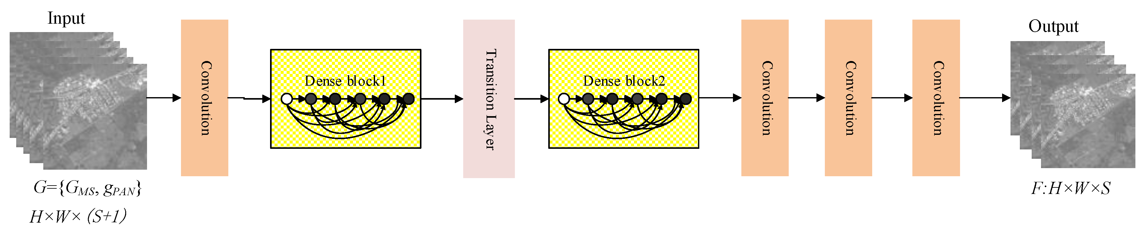
3.1. Improved Dense Block

The original DenseNet-BC architecture was used for image classification. A composite function $H_l(•)$ composed of $1\times 1$ conv and $3\times 3$ conv was used between two convolution layers of this architecture, where conv represents the sequence BN-ReLU-Conv, as shown in Figure 3a. Compared with the image classification, pan-sharpening is an inverse problem that requires the reconstruction of feature maps. Since the BN layer ignores the absolute differences in feature maps and changes the contrast of fused image, the original dense block architecture is not suitable for pan-sharpening. Therefore, this paper proposes an improved dense block that removed the BN layer. The improved dense block not only enhances the spatial resolution of the fused image, but also preserves the same contrast and color as the original MS images in pan-sharpening. Meanwhile, the streamlining of the dense block will reduce the load on computer resources.

The architecture of the dense block designed in this paper is shown in Figure 3b. The proposed composite function $H_{lnew}(•)$ consists of ReLU, $1\times 1$ Conv, ReLU, and $3\times 3$ Conv. The improved dense block is an l-layer ($l=6$) dense block with a growth rate of $k=12$, because a relatively small growth rate can achieve advanced results. Each bottleneck layer produces $4k$ feature maps, and the settings of these hyper-parameters were the same as in [44]. The input layer $x_0$ has $k_0$ feature maps, and each function $H_{lnew}(•)$ will produce k feature maps. Since each layer takes all preceding feature maps as input, the input data of the $l^{\mathrm{th}}$ layer dense block has $(l-1)\times k+k_0$ feature maps.

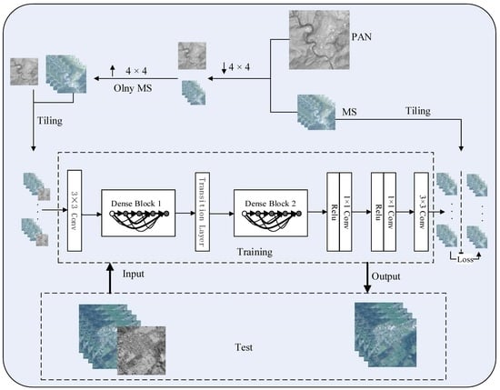
3.2. The Architecture of DCCNP

The proposed network architecture for pan-sharpening is shown in Figure 4 and includes an input layer, an independent convolution layer, two dense blocks, a transition layer, and an output layer. The size of each band of the input layer image is the same as that of each band of the output layer image, but the input layer images have one additional band, i.e., the input layer images have $S+1$ bands compared to the output layer MS images with S bands (which is explained in the next paragraph). The first convolution layer of the DCCNP is an independent convolution layer, which consists of $2k$ convolution kernels with a size of $3\times 3$. After that, the first convolution dense block outputs $7k$ feature maps after the input of $2k$ feature maps through the dense block. Next, to reduce the gradient disappearance, the transition layer is composed of ReLU and has a convolution of size $1\times 1$. A compression factor of $\theta =0.5$ is used to decrease the output of the previous dense blocks and the dimension of the input feature maps of the second dense block. Therefore, the transition layer outputs $\lfloor 7k\theta \rfloor +5k$ feature maps, obtained by the second dense block. Since the feature maps of each convolution layer in the dense block are from all the previous layers, a large number of feature maps is extracted. Because the fused MS images have S bands, we employed two continuous convolution kernels with size of $1\times 1$ to assess the feature map output by the second dense block for dimensionality reduction. The feature maps have their dimensionality as the number of channels in the input feature maps. This dimensionality reduction operation of the proposed DCCNP architecture can effectively extract the features of the PAN image and MS images. The final layer is the image fusion layer, that is the extracted features are convolved through S convolution kernels with the size of $3\times 3$ to obtain the fused MS images.

To better train the proposed DCCNP for pan-sharpening, we constructed a training set containing the high-resolution/low-resolution image patch pairs. Firstly, the low-resolution PAN image $g_{PAN}$ and the MS images of $g_{MS}$ were obtained by spatial blurring and downsampling of the original PAN image ($f_{PAN}$) and the MS image ($f_{MS}$) with S bands. Next, $g_{MS}$ was interpolated to obtain enlarged low-resolution MS images $G_{MS}$, so that the size of each band image was consistent with the size of PAN image $g_{PAN}$ and was then spliced into an $S+1$ band low-resolution image $G=\{G_{MS},g_{PAN}\}$. Next, a slider with a step size of l and window size $h\ast w$ extracted the low-resolution image patches $G^i$ ($i=1,2,\dots ,N$) and high-resolution image patches $f_{MS}^i$ from G and $f_{MS}$, respectively. Thus, we obtained a consistent training set $\{G^i,f_{MS}^i\}$. In the training phase of DCCNP, low-resolution image patches $G^i$ were the input data, and the corresponding fused image patches $F^i$ were obtained through forward propagation with the initial weight. The loss function was used to compute the loss between the pan-sharpened image and the original high-resolution image, and the back propagation algorithm was used to adjust the dense network so that the output fused image block was close to the high-resolution image block. The loss function was the mean square error between the pan-sharpened tile $f_{MS}^i$ and its reference $F^i$ as shown in the training phase of the Figure 2, which is usually expressed by the following Formula (2):

$$L\left(\theta \right)=\frac{1}{N}\sum _{i=1}^N{∥F^i-f_{MS}^i\left(\theta \right)∥}^2$$

(2)

where $\theta$ is the set of all parameters and N is the number of randomly selected patches in one iteration. Because the pixel values of the training images are normalized to (0,1), the value range of loss function is (0,1). The smaller the value, the better the fusion effect and the better the robustness of the proposed architecture of DCCNP.

In summary, the algorithm for solving the proposed model is shown as follows (Algorithm 1).

Algorithm 1 Pan-sharpening by the DCCNP algorithm

Input: The high-resolution PAN image $P_H$ and low-resolution MS images $M_L$ with S bands. Step 1: Given the training set: original PAN image $f_{PAN}$ and MS images $f_{MS}$ with S bands. The low-resolution PAN image $g_{PAN}$ and MS images $g_{MS}$ are obtained by spatial blurring and downsampling of the original PAN image $f_{PAN}$ and MS images $f_{MS}$ with S bands. Step 2: The $g_{MS}$ is interpolated to obtain an enlarged low-resolution MS images $G_{MS}$, so that the size of each band image is consistent with the size of the PAN image $g_{PAN}$ and is then spliced into the $S+1$ band low-resolution images $G=\{G_{MS},g_{PAN}\}$. Step 3: A slider with a step size of l and a window size of $h\times w$ extracts low-resolution image patches $G^i$ ($i=1,2,\dots ,N$) and high-resolution image patches $f_{MS}^i$ from G and $f_{MS}$, respectively. Thus, we obtain the consistent training set $\{G^i,f_{MS}^i\}$ for pixel positions of N. Step 4: Taking $G^i$ as the input data of the first layer of the convolutional neural network, the expected high-resolution image patches $f_{MS}^i$ are obtained according to the initial weight and forward propagation algorithm. Step 5: Using $G^i$ and $f_{MS}^i$, the optimal parameters in the DCCNP architecture were obtained by fine tuning the network according to Formula (2). Step 6: Input the original PAN image $P_H$ and MS images $M_L$; repeat Steps 1 and 2; obtain $(S+1)$-dimensional images G as the input data of the network; load the model; and obtain the desired high-resolution images F. Output: The Pan-sharpened MS images F.

4. Experiment

4.1. Experimental Settings

In order to verify the validity of the DCCNP method in this paper, we employed the remote sensing images from IKONOS and QuickBird satellites for simulation and real experiments. IKONOS satellite is able to capture PAN images at 1 m resolution and MS images at 4m resolution. The experimental data used in this paper came from the remote sensing data collected by the IKONOS satellite sensor in May 2008 in Sichuan, China. The PAN sensor of QuickBird satellite can collect a PAN image with a spatial resolution of 0.7 m, while the MS sensor can simultaneously collect an MS images with a spatial resolution of 2.8 m and four bands. The experimental data were part of the remote sensing image taken of the north island of New Zealand in August 2012.

Due to the scarcity of training sample of remotes sensing images, these images were rotated 90${}^{°}$, 180${}^{°}$, and 270${}^{°}$, respectively, and then, they were cropped into image patches to obtain more experimental data. The experiments included a training stage and a testing stage. According to the experimental datasets used in [35,38], the experimental datasets were divided into training, validation, and test sets. The training and validation sets accounted for a large proportion, and the test set only occupied a small part (as shown in

Table 1. Experimental datasets.

Sensors	Training	Validation	Test
IKONOS	Input: 19,249 $\times (41\times 41\times 5)$	Input: $4096\times (41\times 41\times 5)$	Input: $50\times (250\times 250\times 5)$
	Output: 19,249 $\times (41\times 41\times 4)$	Output: $4096\times (41\times 41\times 4)$	Output: $50\times (250\times 250\times 4)$
QuickBird	Input: 19,249 $\times (41\times 41\times 5)$	Input: $4096\times (41\times 41\times 5)$	Input: $50\times (250\times 250\times 5)$
	Output: 19,249 $\times (41\times 41\times 4)$	Output: $4096\times (41\times 41\times 4)$	Output: $50\times (250\times 250\times 4)$

). The real experiments used thirty image patches with a size of $600\times 600$ from the QuickBird dataset to test the network.

4.2. Simulation Experimental Results and Analysis

4.2.1. Detailed Experimental Implementation

In this paper, the simulation experiment results were compared with four methods, including the adaptive IHS (AIHS) method [46], the à trous wavelet transform (ATWT)-based method [47], PNN [35], and MSDCNN [38]. The parameter settings of these methods were mostly consistent with these references. Specifically, for the PNN model [35], the authors selected different convolution kernels for the experiments, and we only used three convolution kernels with a size of $9\times 9\times 7$, $5\times 5\times 64$, and $5\times 5\times 4$ to extract features from input images, respectively. In the MSDCNN method [38], the training data used in the experiment were the same as those used in this paper, and the input images were PAN image and MS images. However, for the PNN method [35], the input layer contained not only PAN image and MS images, but also included two maps of nonlinear radiometric indices typical of remote sensing.

The pre-processing environment of the experimental data was MATLAB v2016a, and TensorFlow was selected as the development platform for constructing and training the proposed architecture of DCCNP. According to [35], the learning rate of the last two layers was set to ${10}^{-5}$, and that of the other layers was set to ${10}^{-4}$. The batch size was set to 128, and Adam [48] with ${\beta }_1=0.9$ and ${\beta }_2=0.999$ was utilized as the optimizer. For all data settings, the total number of iterations was fixed to $4.51\times {10}^4$.

In order to quantitatively assess the quality of the results, the evaluation criteria generally included subjective evaluation and objective evaluation. For subjective evaluation, the quality of the pan-sharpened image was evaluated by observing the spatial structure information and the degree of color distortion of the pan-sharpened result image, as well as enlarging the local details of the resulting image. For objective evaluation, the following five evaluation criteria were used in this paper: correlation coefficient (CC) [49], root mean squared error (RMSE) [50], erreur relative global adimensionnelle de synthèse (ERGAS) [51], spectral angle mapper (SAM) [52], and the 4-band Universal Image Quality index (Q4) [53]. Specifically, CC refers to the correlation of spectral characteristics between the reference image and pan-sharpened image. The RMSE reflects the difference of the pixel values between the pan-sharpened image and the reference image. ERGAS represents the difference of radiation between the reference image and the pan-sharpened image globally. SAM denotes the angle between the reference image and the spectral vector of the pan-sharpened image. Q reflects the Universal Image Quality index averaged over the bands [54], while Q4 is a 4-band extension of Q.

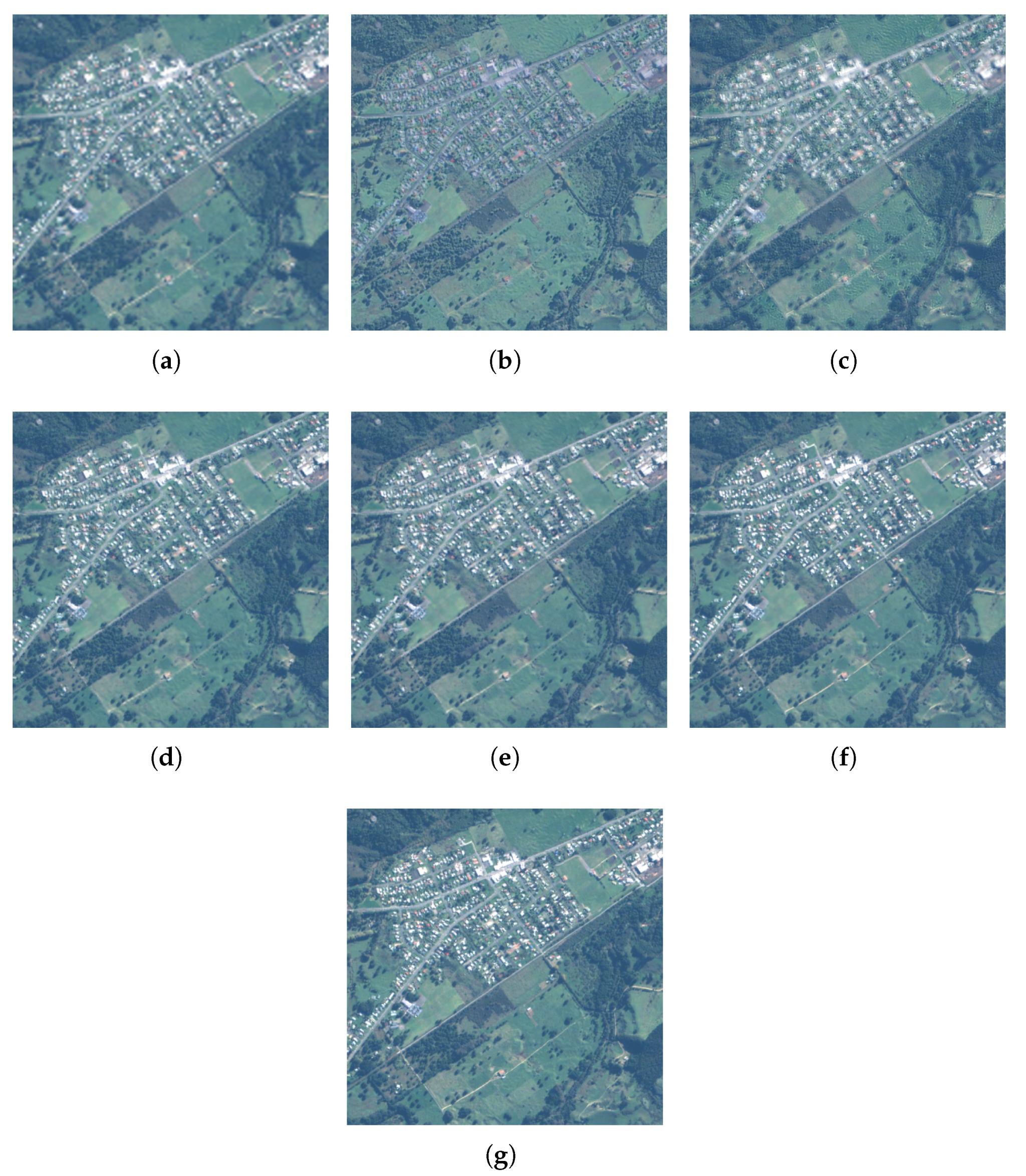
4.2.2. Experiment Using IKONOS Data

The results of five pan-sharpening methods were compared with the input low-resolution MS images, and the original high-resolution MS images were taken as the reference images as shown in Figure 5. Figure 5a is the low-resolution MS images; Figure 5g is the reference image; and Figure 5b–f are the pan-sharpened images of AIHS, ATWT, PNN, MSDCNN, and the proposed method, respectively. These images were false color images, composed of three bands of red, blue, and green. By observing these pan-sharpened images, we found that the spatial structure of Figure 5b was significantly improved, but the spectrum was distorted. Compared with Figure 5b, the color of Figure 5c was greatly improved, but the spatial structure had an obvious blocky aspect. Figure 5d shows a significant improvement in spatial structure restoration and color preservation, but the blocky effect appeared in the spatial structure. Compared with Figure 5d, the spatial structure and color of Figure 5e were greatly improved, but the spatial information was excessively smooth, and the details of the edges and textures lost. Figure 5f is the result of the proposed method. The image was the closest to the reference image both in terms of spatial structure restoration and spectral preservation.

To observe the detail part of the pan-sharpening result images more clearly, we enlarge and display the local area in Figure 5. Figure 6a shows the local area to be enlarged (red rectangle box) in the reference image. Figure 6b–h are an enlarged view of the local area in Figure 5a–g in the red rectangle box. From the magnified images of these local areas, the detail information reconstructed by the method extracted in this paper was clearer and more uniform. To sum up, the results of the proposed methods were better than other fusion methods in the visual effect.

In order to better observe the spectral distortion, Figure 7 shows the difference image between the fused image and the reference image. The red part of the difference image represents the large difference in pixel values, the blue part the small difference, and the green part the middle difference. By observing these difference images, it can be seen that the difference image of the proposed method in this paper (as shown in Figure 7e) was blue in most areas, and the red areas were the least. Therefore, the result image of the proposed method was the closest to the original image, and the fusion effect was slightly better than the comparison methods.

The quantitative assessment values of the IKONOS dataset processed by the different methods are shown in

Table 2. Quantitative assessments of IKONOS data. ERGAS, erreur relative global adimensionnelle de synthèse; SAM, spectral angle mapper.

	AIHS	ATWT	PNN	MSDCNN	DCCNP
$C{C}_{AVG}$	0.7924	0.8819	0.9491	0.9522	0.9616
$RMS{E}_{AVG}$	0.0061	0.0037	0.0016	0.0015	0.0012
ERGAS	3.1983	2.4858	1.6384	1.5794	1.4223
SAM	0.0653	0.0520	0.0322	0.0316	0.0289
$Q_4$	0.7627	0.8211	0.9323	0.9362	0.9480

, where the numbers in black font represent the optimal values of the quantitative assessment. The $C{C}_{AVG}$ and $RMS{E}_{AVG}$ are the average values of $CC$ and $RMSE$, respectively. The experimental results showed that the indexes of the proposed method were better than the other comparison methods.

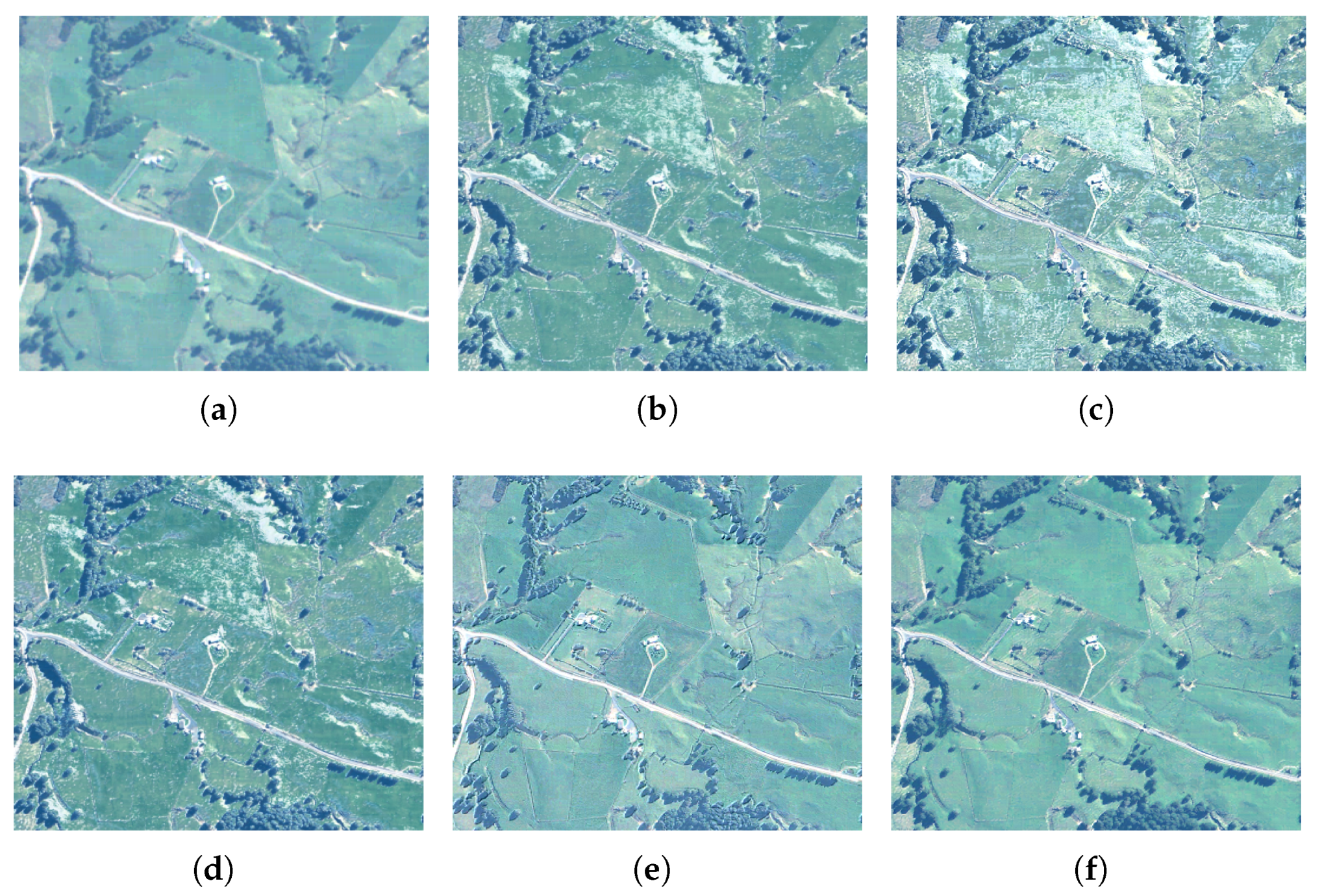
4.2.3. Experiment Using QuickBird Data

To further validate the performance of the proposed algorithm, we continued to carry out simulation experiments using the QuickBird dataset. The pan-sharpened images obtained by the proposed method were compared with those obtained by the other methods as shown in Figure 8. Figure 8a is the input low-resolution image, and Figure 8b–f is the pan-sharpened images obtained by AIHS, ATWT, PNN, MSDCNN, and the proposed method, respectively. It can be seen from Figure 8 that any pan-sharpened images improved the spatial resolution to some extent compared with the input low-resolution MS images and retained the spectral information of the original MS images. After careful observation, we found that the fused image produced by the proposed method gave a clearer visual effect and was closer to the reference image in both terms of spatial resolution and spectral information.

In Figure 9, we enlarge and display the local area in Figure 8. Figure 9a shows the local area to be enlarged (red rectangular box) in the reference image. Figure 9b–h is an enlarged view of the local area in the red rectangular box of Figure 8a–g. In these local area enlarged images, we can see that the detail information recovered by the proposed method was clearer and more uniform.

Figure 10 shows the difference image between the fused image and the reference image. Through observation, it can be found that the difference image produced by the proposed method using IKONOS dataset are consistent with those of QuickBird dataset. Therefore, similar conclusions can be drawn.

The quantitative assessment values of the QuickBird dataset processed by the different methods are shown in

Table 3. Quantitative assessments of IKONOS data.

	AIHS	ATWT	PNN	MSDCNN	DCCNP
$C{C}_{AVG}$	0.8184	0.8412	0.9454	0.9479	0.9754
$RMS{E}_{AVG}$	0.0079	0.0070	0.0020	0.0019	0.0009
ERGAS	4.5807	4.3198	2.4660	2.3835	1.6355
SAM	0.0984	0.0914	0.0483	0.0475	0.0386
$Q_4$	0.8128	0.8223	0.9566	0.9584	0.9790

, where the number in bold font represents the optimal values of each index. The values of Table 3 show that the indexes of the proposed method were better than the other methods.

4.2.4. Comparison of Execution Time

In this subsection, we give the CPU execution time of the above pan-sharpening methods excluding the AIHS and ATWT methods programmed with MATLAB R2016a. PNN, MSDCNN, and the proposed method based on CNN were implemented on the TensorFlow platform and on a PC with i5-7400 3.1 GHz CPU and RAM 8 GB. For the sake of fairness of comparison, the operation parameters are uniformly specified as follows: (a) Each model was trained 300 times. (b) The execution time of PNN, MSDCNN, and the proposed method was divided into two parts: training time and testing time (also named fusion time). (c) The fusion time was obtained by averaging all test images.

The PNN method took about eight hours to train the model because its network architecture was the simplest and it only consisted of three layers. During the test phase, it took about 5.5 s to obtain a pan-sharpened image on average. The proposed method took about 11 h to train the model, which was one hour slower than the MSDCNN method. The reason may be that the network architecture of the proposed method was much deeper, which could extract better spatial-spectral features. The fusion time of the proposed method was about 6.2 s, while the fusion time of the MSDCNN method was about 5.9 s. In general, the execution time of the three methods was roughly the same.

4.3. Real Experimental Results and Analysis

In this section, we use QuickBird data for the real experiments. We input the original PAN image and MS images into the trained network to obtain a pan-sharpened MS images and compared it with other methods for pan-sharpening. The pan-sharpened images are shown in Figure 11. Figure 11a is a bicubic low-resolution MS images, and Figure 11b–f are the pan-sharpened images of AIHS, ATWT, PNN, MSDCNN, and the proposed method, respectively. Through observation, it was found that the proposed method for pan-sharpening was better than other methods in visual effect.

For real experiments, the evaluation criteria adopted the quality with no reference (QNR) [55], which mainly included two parts: spectral distortion $D_{\lambda }$ and spatial distortion $D_s$. We used these three metrics to evaluate the real experimental results quantitatively. The results of the objective evaluation are shown in

Table 4. Quantitative assessments of real experiments on QuickBird data.

	AIHS	ATWT	PNN	MSDCNN	DCCNP
$D_{\lambda }$	0.0966	0.0923	0.0507	0.0543	0.0472
$D_s$	0.0793	0.0833	0.0987	0.0891	0.0784
$ONR$	0.8354	0.8321	0.8592	0.8614	0.8792

, where the number in bold represents the optimal values of the quantitative assessments. As can be seen from the table, the value of the comprehensive assessment index QNR of the proposed method was higher than those of other methods, indicating that the pan-sharpened result was the best.

4.4. Discussion of the BN Layer

In this section, we continue to discuss the role of the improved dense block in the DCCNP network and the effect of bottleneck layers and compression factors after the dense block. In order to verify the effectiveness of the proposed method, we performed three experiments on IKONOS and QuickBird data. The first experiment (named DCCNP) was to use the network architectural proposed in this paper, including an independent convolutional layer, two dense blocks, a transition layer, two bottleneck layers with the compression factors, and a reconstruction layer. The second experiment (named DCCNP + BN) was to change the dense block of the first experiment to the original dense block (i.e., the original dense block contained the BN layer), and the others remained unchanged. The third experiment (named DCCNP-BC) did not use two bottleneck layers and compression factors of DCCNP architecture, and the others were unchanged. The batch size was set to 128, and Adam with ${\beta }_1=0.9$ and ${\beta }_2=0.999$ was utilized as the optimizer. For all experiments, the total number of iterations was fixed to $4.51\times {10}^4$. The quantitative evaluation results of IKONOS and QuickBird are shown in

Table 5. Quantitative assessments of different experiment on the IKONOS data. BC, bottleneck layer and compression factor.

	${\mathit{C}\mathit{C}}_{\mathit{A}\mathit{V}\mathit{G}}$	${\mathit{R}\mathit{M}\mathit{S}\mathit{E}}_{\mathit{A}\mathit{V}\mathit{G}}$	ERGAS	SAM	${\mathit{Q}}_4$
$DCCNP$	0.9616	0.0012	1.4223	0.0289	0.9480
$DCCNP+BN$	0.9501	0.0015	1.5246	0.0308	0.9364
$DCCNP-BC$	0.9585	0.0014	1.4763	0.0257	0.9387

and

Table 6. Quantitative assessments of different experiment on the QuickBird data.

	${\mathit{C}\mathit{C}}_{\mathit{A}\mathit{V}\mathit{G}}$	${\mathit{R}\mathit{M}\mathit{S}\mathit{E}}_{\mathit{A}\mathit{V}\mathit{G}}$	ERGAS	SAM	${\mathit{Q}}_4$
$DCCNP$	0.9754	0.0009	1.6355	0.0386	0.9790
$DCCNP+BN$	0.9547	0.0018	1.5246	0.0425	0.9578
$DCCNP-BC$	0.9684	0.0012	1.4763	0.0317	0.9687

, respectively. The best results of each index are highlighted in bold.

By comparing the results of DCCNP and DCCNP+BN in the two tables, we can see that the results of DCCNP were better than the results of DCCNP+BN on each evaluation index. DCCNP used the dense block without the BN layer, and DCCNP+BN used the original dense block with the BN layer. Through the comparison, we could conclude that the improved dense block without the BN layer was more suitable for pan-sharpening than the original dense block.

Through the comparison of DCCNP and DCCNP-BC, it was obvious that the results of the DCCNP were superior to the results of DCCNP-BC in all aspects. Therefore, we could conclude that the proposed method using the bottleneck layers and compression factors could effectively prevent the loss of fusion information and make the fusion image much clearer.

5. Conclusions

In view of the particularities of pan-sharpening, this paper proposed a new method that applied DCCNP to remote sensing images. This method increased the flexibility and diversity of the network by utilizing the advantages of DCCNP, such as feature reuse and enhanced feature propagation. To extract more spatial feature information from the PAN image and more spectral characteristics of the MS images, a dense block was added to the convolution network to deepen the network depth; MS images with rich spectral information and high spatial resolution were thus obtained. An analysis of the experimental results revealed that the pan-sharpened image obtained by the proposed method was not only subjectively visually enhanced, but was also optimal in terms of the objective evaluation criteria.

In the near future, the proposed method will be implemented on parallel computing platforms, such as a GPU [56,57] or a multi-core CPU [58], to accelerate the speed for pan-sharpening. The latest architecture of deep neural networks, such as the generative adversarial network (GAN) and its derived structures [59], will be explored to extract better spatial and spectral features to lead to the highest quality pan-sharpened results.

References

1. Sun, L.; Ma, C.; Chen, Y.; Shim, H.J.; Wu, Z.; Jeon, B. Adjacent superpixel-based multiscale spatial-spectral kernel for hyperspectral classification. IEEE J. Sel. Top. Appl. Earth Obs. Remote Sens. 2019, 312, 1905–1919. [Google Scholar] [CrossRef]
2. Wu, Z.; Zhu, W.; Chanussot, J.; Xu, Y.; Osher, S. Hyperspectral anomaly detection via global and local joint modeling of background. IEEE Trans. Signal Process. 2019, 67, 3858–3869. [Google Scholar] [CrossRef]
3. Sun, L.; Ge, W.; Chen, Y.; Zhang, J.; Jeon, B. Hyperspectral unmixing employing l1-l2 sparsity and total variation regularization. Inter. J. Remote Sens. 2018, 39, 6037–6060. [Google Scholar] [CrossRef]
4. Xu, Y.; Wu, Z.; Chanussot, J.; Wei, Z. Nonlocal patch tensor sparse representation for hyperspectral image super-resolution. IEEE Trans. Image Process. 2019, 28, 3034–3047. [Google Scholar] [CrossRef] [PubMed]
5. Loncan, L.; De Almeida, L.B.; Bioucas-Dias, J.M.; Briottet, X.; Chanussot, J.; Dobigeon, N.; Fabre, S.; Liao, W.; Licciardi, G.A.; Simões, M.; et al. Hyperspectral Pansharpening: A Review. IEEE Trans. Geosci. Remote Sens. Mag. 2015, 3, 27–46. [Google Scholar] [CrossRef] [Green Version]
6. Zhao, C.; Gao, X.; Emery, W.J.; Wang, Y.; Li, J. An integrated spatio-spectral temporal sparse representation method for fusing remote-sensing images with different resolutions. IEEE Trans. Geosci. Remote Sens. 2018, 56, 3358–3370. [Google Scholar] [CrossRef]
7. Scarpa, G.; Vitale, S.; Cozzolino, D. Target-adaptive CNN-based pansharpening. IEEE Trans. Geosci. Remote Sens. 2018, 56, 5443–5457. [Google Scholar] [CrossRef] [Green Version]
8. Lolli, S.; Alparone, L.; Garzelli, A.; Vivone, G. Benefits of haze removal for modulation-based pansharpening. In Proceedings of the Image and Signal Processing for Remote Sensing, Warsaw, Poland, 4–6 Octobor 2017. [Google Scholar]
9. Gaetano, R.; Masi, G.; Poggi, G.; Verdoliva, L.; Scarpa, G. Marker-controlled watershed-based segmentation of multiresolution remote sensing images. IEEE Trans. Geosci. Remote Sens. 2015, 53, 2987–3004. [Google Scholar] [CrossRef]
10. Ayhan, E.; Atay, G. Spectral and spatial quality analysis in pan sharpening process. J. Indian Soc. Remote Sens. 2011, 40, 379–388. [Google Scholar] [CrossRef]
11. Wang, M.; Zhang, J.; Cao, D. Fusion of multispectral and panchromatic satellite images based on ihs and curvelet transformations. In Proceedings of the 2007 International Conference on Wavelet Analysis and Pattern Recognition, Beijng, China, 2–4 November 2007. [Google Scholar]
12. Zhu, X.; Bao, W. Comparison of remote sensing image fusion strategies adopted in HSV and IHS. Int. J. Remote Sens. 2017, 46, 377–385. [Google Scholar] [CrossRef]
13. Pohl, C.; Van Genderen, J. Review article multisensor image fusion in remote sensing: Concepts, methods and applications. J. Indian Soc. Remote Sens. 1998, 19, 823–854. [Google Scholar] [CrossRef] [Green Version]
14. Choi, J.; Yu, K.; Kim, Y. A new adaptive component-substitution-based satellite image fusion by using partial replacement. IEEE Trans. Geosci. Remote Sens. 2011, 49, 295–309. [Google Scholar] [CrossRef]
15. Laporterie, F.; Flouzat, G. The morphological pyramid concept as a tool for multi-resolution data fusion in remote sensing. Integr. Comput. Aided Eng. 2003, 10, 63–79. [Google Scholar] [CrossRef]
16. Amro, I.; Mateos, J. Multispectral image pansharpening based on the contourlet transform. Inf. Opt. Photonics 2010, 206, 247–261. [Google Scholar]
17. Panchal, S.; Thakker, R. Contourlet transform with sparse representation-based integrated approach for image pansharpening. IETE J. Res. 2017, 56, 1–11. [Google Scholar] [CrossRef]
18. Yang, Y.; Que, Y.; Huang, S.; Lin, P. Multimodal sensor medical image fusion based on type-2 fuzzy logic in NSCT domain. IEEE Sens. J. 2016, 1–10. [Google Scholar] [CrossRef]
19. Liu, Y.; Liu, S.; Wang, Z. A general framework for image fusion based on multi-scale transform and sparse representation. Inf. Fusion 2015, 24, 147–164. [Google Scholar] [CrossRef]
20. Wu, Z.; Huang, Y.; Zhang, K. Remote sensing image fusion method based on PCA and curvelet transform. J. Indian Soc. Remote Sens. 2018, 46, 687–695. [Google Scholar] [CrossRef]
21. Moghadam, F.; Shahdoosti, H. A new multifocus image fusion method using contourlet transform. arXiv 2017, arXiv:1709.09528. [Google Scholar]
22. Liu, J.; Zhang, J.; Du, Y. A fusion method of multi-spectral image and panchromatic image based on NSCT transform and adaptive Gamma correction. In Proceedings of the 3rd International Conference on Information Systems Engineering (ICISE), Shanghai, China, 4–6 May 2018. [Google Scholar]
23. Lim, W.Q. The discrete shearlet transform: A new directional transform and compactly supported shearlet frames. IEEE Trans. Image Process. 2010, 19, 1166–1180. [Google Scholar]
24. Sheng, D.; Wu, Y. Method of remote sensing image enhancement in NSST domain based on multi-stages particle swarm optimization. In Proceedings of the 2nd International Conference on Multimedia and Image Processing (ICMIP), Wuhan, China, 17–19 March 2017. [Google Scholar]
25. Song, Y.; Yang, G.; Xie, H.; Zhang, D.; Sun, X. Residual domain dictionary learning for compressed sensing video recovery. Multimed. Tools Appl. 2017, 76, 10083–10096. [Google Scholar] [CrossRef]
26. Li, S.; Yang, B. A new pan-sharpening method using a compressed sensing technique. IEEE Trans. Geosci. Remote Sens. 2011, 49, 738–746. [Google Scholar] [CrossRef]
27. Jiang, C.; Zhang, H.; Shen, H.; Zhang, L. A practical compressed sensing-based pan-sharpening method. IEEE Trans. Geosci. Remote Sens. 2012, 9, 629–633. [Google Scholar] [CrossRef]
28. Li, S.; Yin, H.; Fang, L. Remote sensing image fusion via sparse representations over learned dictionaries. IEEE Trans. Image Process. 2013, 51, 4779–4789. [Google Scholar] [CrossRef]
29. Guo, M.; Zhang, H.; Li, J.; Zhang, L.; Shen, H. An online coupled dictionary learning approach for remote sensing image fusion. IEEE J. Sel. Top. Appl. Earth Obs. Remote Sens. 2014, 7, 1284–1294. [Google Scholar] [CrossRef]
30. Zhu, X.; Bamler, R. A sparse image fusion algorithm with application to pan-sharpening. IEEE Trans. Geosci. Remote Sens. 2013, 51, 2827–2836. [Google Scholar] [CrossRef]
31. Long, M.; Yan, Z. Detecting Iris liveness with batch normalized convolutional neural network. Comput. Mater. Contin. 2019, 58, 493–504. [Google Scholar] [CrossRef]
32. Zeng, D.; Dai, Y.; Li, F.; Sherratt, R.; Wang, J. Adversarial learning for distant dupervised relation extraction. Comput. Mater. Contin. 2018, 55, 121–136. [Google Scholar]
33. Zhou, S.; Ke, M.; Luo, P. Multi-camera transfer GAN for person re-dentification. J. Vis. Commun. Image Remote 2019, 59, 393–400. [Google Scholar] [CrossRef]
34. Huang, W.; Xiao, L.; Wei, Z.; Liu, H.; Tang, S. A new pan-sharpening method with deep neural networks. IEEE Geosc. Remote Sens. Lett. 2015, 12, 1037–1041. [Google Scholar] [CrossRef]
35. Masi, G.; Cozzolino, D.; Verdoliva, L.; Scarpa, G. Pansharpening by convolutional neural networks. Remote Sens. 2016, 8, 594. [Google Scholar] [CrossRef] [Green Version]
36. Meng, R.; Rice, S.G.; Wang, J.; Sun, X. A fusion steganographic algorithm based on faster R-CNN. Comput. Mater. Contin. 2018, 55, 1–16. [Google Scholar]
37. Rao, Y.; He, L.; Zhu, J. A residual convolutional neural network for pan-shaprening. In Proceedings of the 2017 International Workshop on Remote Sensing with Intelligent Processing (RSIP), Shanghai, China, 18–21 May 2017. [Google Scholar]
38. Yuan, Q.; Wei, Y.; Meng, X.; Shen, H.; Zhang, L. A multiscale and multidepth convolutional neural network for remote sensing imagery Pan-sharpening. IEEE J. Sel. Top. Appl. Earth Obs. Remote Sens. 2018, 11, 978–989. [Google Scholar] [CrossRef] [Green Version]
39. Tsagkatakis, G.; Aidini, A.; Fotiadou, K.; Giannopoulos, M.; Pentari, A.; Tsakalides, P. Survey of deep-learning approaches for remote sensing observation enhancement. Sensors 2019, 29, 3929. [Google Scholar] [CrossRef] [Green Version]
40. Wang, W.; Jiang, Y.; Luo, Y.; Ji, L.; Wang, X.; Zhang, T. An advanced deep residual dense network (DRDN) approach for image super-resolution. Int. J. Comput. Int. Syst. 2019, 12, 1592–1601. [Google Scholar]
41. Dong, C.; Loy, C.; He, K.; Tang, X. Learning a deep convolutional network for image super-resolution. In Proceedings of the European Conference on Computer Vision, Zurich, Switzerland, 6–12 September 2014. [Google Scholar]
42. Wald, L.; Ranchin, T.; Mangolini, M. Fusion of satellite images of different spatial resolution: Assessing the quality of resulting images. Photogramm. Eng. Remote Sens. 1997, 63, 691–699. [Google Scholar]
43. Zeng, D.; Dai, Y.; Li, F.; Wang, J.; Sangaiah, A.K. Aspect based sentiment analysis by a linguistically regularized CNN with gated mechanism. J. Intell. Fuzzy Syst. 2019, 36, 3971–3980. [Google Scholar] [CrossRef]
44. Huang, G.; Liu, Z.; Van Der Maaten, L.; Weinberger, K.Q. Densely connected convolutional networks. In Proceedings of the 2017 IEEE Conference on Computer Vision and Pattern Recognition (CVPR), Honolulu, HI, USA, 21–26 July 2017; pp. 2261–2269. [Google Scholar]
45. Luo, Y.; Qin, J.; Xiang, X.; Tan, Y.; Liu, Q.; Xiang, L. Coverless real-time image information hiding based on image block matching and dense convolutional network. J. Real-Time Image Process. 2020, 17, 125–135. [Google Scholar] [CrossRef]
46. Rahmani, S.; Strait, M.; Merkurjev, D.; Moeller, M.; Wittman, T. An Adaptive IHS Pan-Sharpening Method. IEEE Geosci. Remote Sci. 2010, 7, 746–750. [Google Scholar] [CrossRef] [Green Version]
47. Nunez, J.; Otazu, X.; Fors, O.; Prades, A.; Pala, V.; Arbiol, R. Multiresolution-based image fusion with additive wavelet decomposition. IEEE Trans. Geosci. Remote Sens. 1999, 37, 1204–1211. [Google Scholar] [CrossRef] [Green Version]
48. Kingma, D.; Ba, J. Adam: A Method for Stochastic Optimization. Available online: https://arxiv.org/pdf/1412.6980.pdf (accessed on 2 April 2020).
49. Zhou, J.; Civco, D.L.; Silander, J.A. A wavelet transform method to merge Landsat TM and SPOT panchromatic data. Int. J. Remote Sens. 1998, 19, 743–757. [Google Scholar] [CrossRef]
50. Liu, Z.; Blasch, E.; Xue, Z.; Zhao, J.; Laganiere, R.; Wu, W. Objective assessment of multiresolution image fusion algorithms for context enhancement in night vision: A comparative study. IEEE Trans. Pattern Anal. 2012, 34, 94–109. [Google Scholar] [CrossRef] [PubMed]
51. Wald, L. Data Fusion: Definitions and Architectures-Fusion of Images of Different Spatial Resolutions; Presses desMines: Paris, France, 2002; pp. 135–141. [Google Scholar]
52. Yuhas, R.H.; Goetz, A.F.H.; Boardman, J.W. Discrimination among semi-arid landscape endmembers usingthe Spectral AngleMapper (SAM) algorithm. In Proceedings of the Summaries of the Third Annual JPL Airborne GeoscienceWorkshop, AVIRIS Workshop, Pasadena, CA, USA, 1–5 June 1992. [Google Scholar]
53. Alparone, L.; Baronti, S.; Garzelli, A.; Nencini, F. A global quality measurement of Pan-sharpened multispectral imagery. IEEE Geosci. Remote Sens. Lett. 2004, 1, 313–317. [Google Scholar] [CrossRef]
54. Wang, Z.; Bovik, A. A universal image quality index. IEEE Signal Process. Lett. 2002, 9, 81–84. [Google Scholar] [CrossRef]
55. Alparone, L.; Aiazzi, B.; Baronti, S.; Garzelli, A.; Nencini, F.; Selva, M. Multispectral and panchromatic data fusion assessment without reference. Photogram Eng. Remote Sens. 2008, 74, 1204–1211. [Google Scholar] [CrossRef] [Green Version]
56. Wu, Z.; Liu, J.; Ye, S.; Sun, L.; Wei, Z. Optimization of minimum volume constrained hyperspectral image unmixing on CPU-GPU heterogeneous platform. J. Real-Time Image Process. 2018, 15, 265–277. [Google Scholar] [CrossRef]
57. Wu, Z.; Shi, L.; Li, J.; Wang, Q.; Sun, L.; Wei, Z.; Plaza, J.; Plaza, A. GPU Parallel Implementation of Spatially Adaptive Hyperspectral Image Classification. IEEE J. Sel. Top. Appl. Earth Obs. Remote Sens. 2018, 11, 1131–1143. [Google Scholar] [CrossRef]
58. Jiang, Y.; Zhao, M.; Hu, C.; He, L.; Bai, H.; Wang, J. A parallel FP-growth algorithm on World Ocean Atlas data with multi-core CPU. J. Supercomput. 2019, 75, 732–745. [Google Scholar] [CrossRef]
59. Tu, Y.; Lin, Y.; Wang, J.; Kim, J.U. Semi-supervised learning with Generative Adversarial Networks on digital signal modulation classification. Comput. Mater. Contin. 2018, 55, 243–254. [Google Scholar]
Figure 1. A five-layer dense block with a growth rate of k = 4 . All preceding feature-maps are the input data of each layer.
Ijgi 09 00242 g001
Figure 2. The framework of the densely connected convolutional networks for pan-sharpening (DCCNP) method.
Ijgi 09 00242 g002
Figure 3. Comparison of the dense block between the original network and the proposed network.
Ijgi 09 00242 g003
Figure 4. The architecture of DCCNP for pan-sharpening.
Ijgi 09 00242 g004
Figure 5. IKONOS original images and Pan-sharpened images by different methods. (a) Low-resolution MS; (b) adaptive IHS (AIHS); (c) à trous wavelet transform (ATWT); (d) pan-sharpening neural network (PNN); (e) multi-scale and multi-depth convolution neural network (MSDCNN); (f) the proposed method; (g) ground truth.
Ijgi 09 00242 g005
Figure 6. (a) Red rectangle area to be enlarged in the reference image. (bh) are partial enlarged views of Figure 5a–g.
Ijgi 09 00242 g006
Figure 7. The difference image between the pan-sharpened image and the reference image of the IKONOS data, where red represents the large difference, blue the small difference, and green the middle difference. (a) AIHS; (b) ATWT; (c) PNN; (d) MSDCNN; (e) the proposed method.
Ijgi 09 00242 g007
Figure 8. QuickBird original images and Pan-sharpened images by different methods. (a) Low-resolution MS; (b) AIHS; (c) ATWT; (d) PNN; (e) MSDCNN; (f) the proposed method; (g) ground truth.
Ijgi 09 00242 g008
Figure 9. (a) Red rectangle area to be enlarged in the reference image. (bh) are partial enlarged views of Figure 8a–g.
Ijgi 09 00242 g009
Figure 10. The difference image between the result image and the reference image of the QuickBird data. (a) AIHS, (b) ATWT, (c) PNN, (d) MSDCNN, (e) the proposed method.
Ijgi 09 00242 g010
Figure 11. Real experimental results by different methods on QuickBird data. (a) Low-resolution MS images; (b) AIHS; (c) ATWT; (d) PNN; (e) MSDCNN; (f) the proposed method.
Ijgi 09 00242 g011