CostNet: A Concise Overpass Spatiotemporal Network for Predictive Learning


Abstract
1. Introduction
2. Related Work
3. Preliminaries
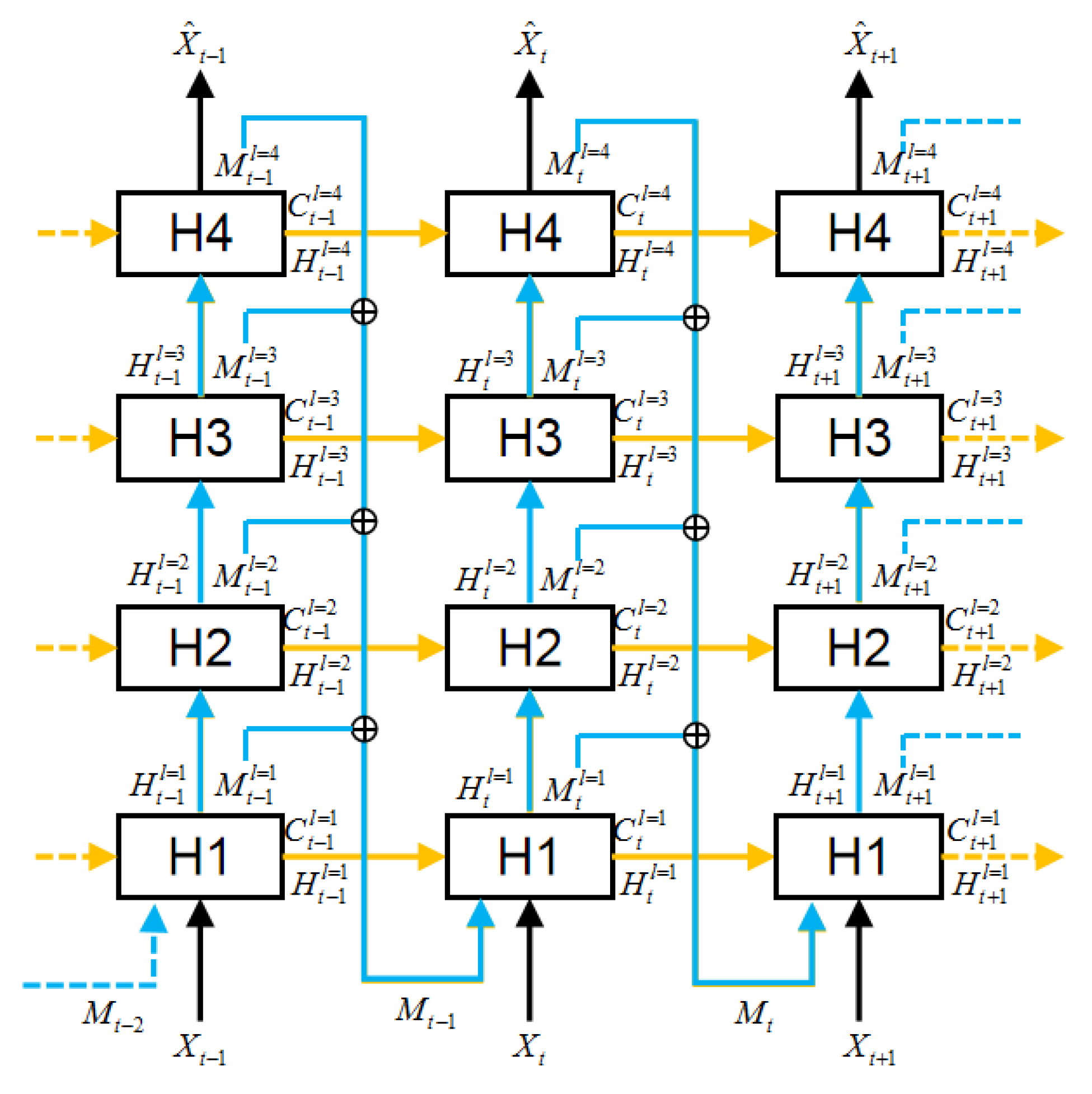
4. Methodology
4.1. Horizon LSTM
4.2. Vertical Structure
5. Experiments
5.1. Moving MNIST Dataset
5.1.1. Implementation
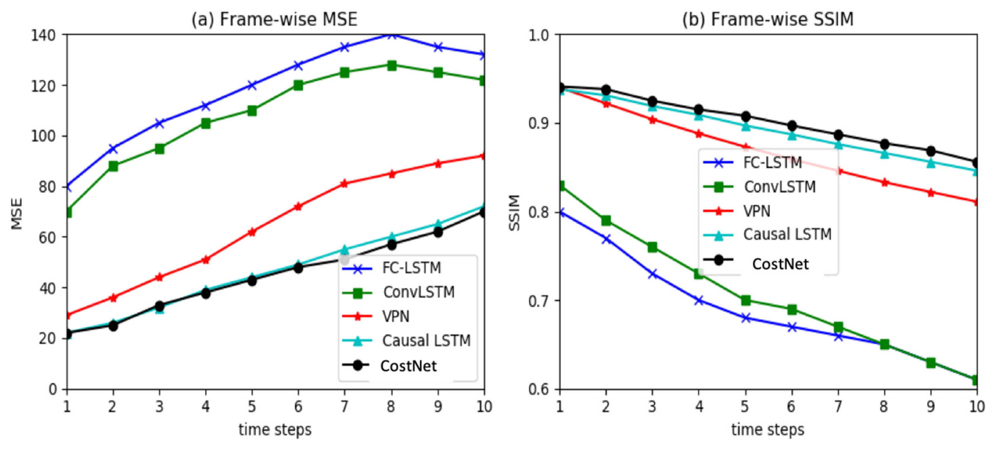
5.1.2. Results
5.2. Radar Echo Dataset
5.2.1. Implementation
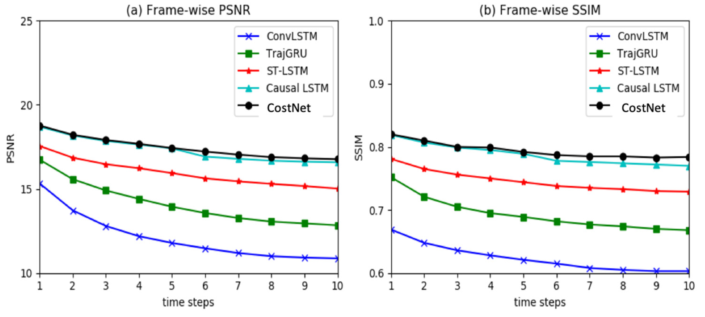
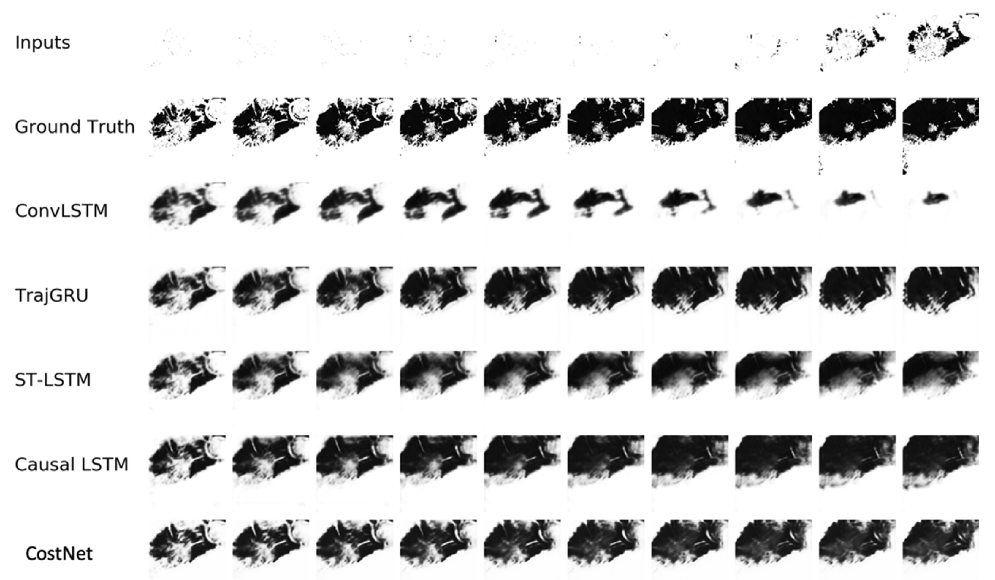
5.2.2. Results
6. Conclusions and Future Work
Author Contributions
Funding
Conflicts of Interest
References
- Wang, M.; Zhang, X.; Niu, X.; Wang, F.; Zhang, X. Scene classification of high-resolution remotely sensed image based on resnet. J. Geov. Spatial Anal. 2019, 3, 16. [Google Scholar] [CrossRef]
- Wang, S.; Zhong, Y.; Wang, E. An integrated GIS platform architecture for spatiotemporal big data. Future Gener. Comput. Syst. 2019, 94, 160–172. [Google Scholar] [CrossRef]
- Liu, K.; Gao, S.; Qiu, P.; Liu, X.; Yan, B.; Lu, F. Road2vec: Measuring traffic interactions in urban road system from massive travel routes. ISPRS Int. J. Geo Inf. 2017, 6, 321. [Google Scholar] [CrossRef]
- Liu, Y.; Cao, G.; Zhao, N. Integrate machine learning and geostatistics for high-resolution mapping of ground-level pm2. 5 concentrations. In Spatiotemporal Analysis of Air Pollution and Its Application in Public Health; Elsevier: Amsterdam, The Netherlands, 2020; pp. 135–151. [Google Scholar]
- Li, H.; Liu, J.; Zhou, X. Intelligent map reader: A framework for topographic map understanding with deep learning and gazetteer. IEEE Access 2018, 6, 25363–25376. [Google Scholar] [CrossRef]
- LeCun, Y. Predictive learning. Proc. Speech NIPS 2016. Available online: https://drive.google.com/file/d/0BxKBnD5y2M8NREZod0tVdW5FLTQ/view (accessed on 12 March 2020).
- Xingjian, S.; Chen, Z.; Wang, H.; Yeung, D.-Y.; Wong, W.-K.; Woo, W.-C. Convolutional lstm network: A machine learning approach for precipitation nowcasting. In Proceedings of the Advances in Neural Information Processing Systems, Montréal, QC, Canada, 12–17 December 2015; pp. 802–810. [Google Scholar]
- Shi, X.; Gao, Z.; Lausen, L.; Wang, H.; Yeung, D.-Y.; Wong, W.-k.; Woo, W.-C. Deep learning for precipitation nowcasting: A benchmark and a new model. In Proceedings of the Advances in Neural Information Processing Systems, Long Beach, CA, USA, 4–9 December 2017; pp. 5617–5627. [Google Scholar]
- Wang, Y.; Long, M.; Wang, J.; Gao, Z.; Philip, S.Y. Predrnn: Recurrent neural networks for predictive learning using spatiotemporal lstms. In Proceedings of the Advances in Neural Information Processing Systems, Long Beach, CA, USA, 4–9 December 2017; pp. 879–888. [Google Scholar]
- Zhang, J.; Zheng, Y.; Qi, D.; Li, R.; Yi, X. DNN-based prediction model for spatio-temporal data. In Proceedings of the 24th ACM SIGSPATIAL International Conference on Advances in Geographic Information Systems, Burlingame, CA, USA, 31 October–3 November 2016; ACM: Burlingame, CA, USA, 2016; pp. 1–4. [Google Scholar]
- Xu, Z.; Wang, Y.; Long, M.; Wang, J.; KLiss, M. PredCNN: Predictive learning with cascade convolutions. In Proceedings of the Twenty-Seventh International Joint Conference on Artificial Intelligence (IJCAI-18), Stockholm, Sweden, 13–19 July 2018; pp. 2940–2947. [Google Scholar]
- Zhang, J.; Zheng, Y.; Qi, D. Deep spatio-temporal residual networks for citywide crowd flows prediction. In Proceedings of the Thirty-First AAAI Conference on Artificial Intelligence, San Francisco, CA, USA, 4–10 February 2017. [Google Scholar]
- Oliu, M.; Selva, J.; Escalera, S. Folded recurrent neural networks for future video prediction. In Proceedings of the European Conference on Computer Vision (ECCV), Munich, Germany, 8–14 September 2018; pp. 716–731. [Google Scholar]
- Ranzato, M.; Szlam, A.; Bruna, J.; Mathieu, M.; Collobert, R.; Chopra, S. Video (language) modeling: A baseline for generative models of natural videos. arXiv 2014, arXiv:1412.6604. [Google Scholar]
- Lotter, W.; Kreiman, G.; Cox, D. Deep predictive coding networks for video prediction and unsupervised learning. arXiv 2016, arXiv:1605.08104. [Google Scholar]
- Kalchbrenner, N.; van den Oord, A.; Simonyan, K.; Danihelka, I.; Vinyals, O.; Graves, A.; Kavukcuoglu, K. Video pixel networks. In Proceedings of the 34th International Conference on Machine Learning-Volume 70; JMLR: Sydney, Australia, 2017; pp. 1771–1779. [Google Scholar]
- Mathieu, M.; Couprie, C.; LeCun, Y. Deep multi-scale video prediction beyond mean square error. arXiv 2015, arXiv:1511.05440. [Google Scholar]
- Jain, A.; Zamir, A.R.; Savarese, S.; Saxena, A. Structural-rnn: Deep learning on spatio-temporal graphs. In Proceedings of the IEEE Conference on Computer Vision and Pattern Recognition, Las Vegas, NV, USA, 26 June–1 July 2016; pp. 5308–5317. [Google Scholar]
- Tran, D.; Bourdev, L.D.; Fergus, R.; Torresani, L.; Paluri, M. C3D: Generic features for video analysis. CoRR abs/1412.0767 2014, 2, 8. [Google Scholar]
- LeCun, Y.; Bengio, Y.; Hinton, G. Deep learning. Nature 2015, 521, 436–444. [Google Scholar] [CrossRef] [PubMed]
- Bengio, Y.; Simard, P.; Frasconi, P. Learning long-term dependencies with gradient descent is difficult. IEEE Trans. Neural Netw. 1994, 5, 157–166. [Google Scholar] [CrossRef] [PubMed]
- Williams, R.J.; Zipser, D. Gradient-based learning algorithms for recurrent. In Backpropagation: Theory, Architectures, and Applications; Psychology Press: Brighton, UK, 1995; Volume 433. [Google Scholar]
- Pascanu, R.; Mikolov, T.; Bengio, Y. On the difficulty of training recurrent neural networks. In Proceedings of the International conference on machine learning, Atlanta, GA, USA, 16–21 June 2013; pp. 1310–1318. [Google Scholar]
- He, K.; Zhang, X.; Ren, S.; Sun, J. Deep residual learning for image recognition. In Proceedings of the IEEE Conference on Computer Vision and Pattern Recognition, Las Vegas, NV, USA, 26 June–1 July 2016; pp. 770–778. [Google Scholar]
- LeCun, Y.; Bottou, L.; Bengio, Y.; Haffner, P. Gradient-based learning applied to document recognition. Proc. IEEE 1998, 86, 2278–2324. [Google Scholar] [CrossRef]
- Jordan, M.I. Serial order: A parallel distributed processing approach. In Advances in Psychology; Elsevier: Amsterdam, The Netherlands, 1997; Volume 121, pp. 471–495. [Google Scholar]
- Hochreiter, S.; Schmidhuber, J. Long short-term memory. Neural Comput. 1997, 9, 1735–1780. [Google Scholar] [CrossRef] [PubMed]
- Goodfellow, I.; Pouget-Abadie, J.; Mirza, M.; Xu, B.; Warde-Farley, D.; Ozair, S.; Courville, A.; Bengio, Y. Generative adversarial nets. In Proceedings of the Advances in Neural Information Processing Systems, Montréal, QC, Canada, 8–13 December 2014; pp. 2672–2680. [Google Scholar]
- Denton, E.L.; Chintala, S.; Fergus, R. Deep generative image models using a laplacian pyramid of adversarial networks. In Proceedings of the Advances in Neural Information Processing Systems, Montréal, QC, Canada, 7–12 December 2015; pp. 1486–1494. [Google Scholar]
- Oh, J.; Guo, X.; Lee, H.; Lewis, R.L.; Singh, S. Action-conditional video prediction using deep networks in atari games. In Proceedings of the Advances in neural information processing systems, Montréal, QC, Canada, 7–12 December 2015; pp. 2863–2871. [Google Scholar]
- Jia, X.; De Brabandere, B.; Tuytelaars, T.; Gool, L.V. Dynamic filter networks. In Proceedings of the Advances in Neural Information Processing Systems, Barcelona Spain, 5–10 December 2016; pp. 667–675. [Google Scholar]
- Villegas, R.; Yang, J.; Zou, Y.; Sohn, S.; Lin, X.; Lee, H. Learning to generate long-term future via hierarchical prediction. In Proceedings of the 34th International Conference on Machine Learning-Volume 70; JMLR: Sydney, Australia, 2017; pp. 3560–3569. [Google Scholar]
- Srivastava, N.; Mansimov, E.; Salakhudinov, R. Unsupervised learning of video representations using LSTMs. In Proceedings of the International conference on machine learning, Lille, France, 6–11 July 2015; pp. 843–852. [Google Scholar]
- Finn, C.; Goodfellow, I.; Levine, S. Unsupervised learning for physical interaction through video prediction. In Proceedings of the Advances in neural information processing systems, Barcelona, Spain, 5–10 December 2016; pp. 64–72. [Google Scholar]
- Patraucean, V.; Handa, A.; Cipolla, R. Spatio-temporal video autoencoder with differentiable memory. arXiv 2015, arXiv:1511.06309. [Google Scholar]
- Villegas, R.; Yang, J.; Hong, S.; Lin, X.; Lee, H. Decomposing motion and content for natural video sequence prediction. arXiv 2017, arXiv:1706.08033. [Google Scholar]
- Wang, Y.; Gao, Z.; Long, M.; Wang, J.; Yu, P.S. PredRNN++: Towards a resolution of the deep-in-time dilemma in spatiotemporal predictive learning. arXiv 2018, arXiv:1804.06300. [Google Scholar]
- Vondrick, C.; Pirsiavash, H.; Torralba, A. Generating videos with scene dynamics. In Proceedings of the Advances In Neural Information Processing Systems, Barcelona, Spain, 5–10 December 2016; pp. 613–621. [Google Scholar]
- Lu, C.; Hirsch, M.; Scholkopf, B. Flexible spatio-temporal networks for video prediction. In Proceedings of the IEEE Conference on Computer Vision and Pattern Recognition, Honolulu, HI, USA, 21–26 July 2017; pp. 6523–6531. [Google Scholar]
- Denton, E.L. Unsupervised learning of disentangled representations from video. In Proceedings of the Advances in Neural Information Processing Systems, Long Beach, CA, USA, 4–9 December 2017; pp. 4414–4423. [Google Scholar]
- Bhattacharjee, P.; Das, S. Temporal coherency based criteria for predicting video frames using deep multi-stage generative adversarial networks. In Proceedings of the Advances in Neural Information Processing Systems, Long Beach, CA, USA, 4–9 December 2017; pp. 4268–4277. [Google Scholar]
- Chollet, F. Keras: The python deep learning library. Available online: https://keras.io/#support (accessed on 12 March 2020).
- Abadi, M.; Agarwal, A.; Barham, P.; Brevdo, E.; Chen, Z.; Citro, C.; Corrado, G.S.; Davis, A.; Dean, J.; Devin, M. Tensorflow: Large-Scale Machine Learning on Heterogeneous Systems. arXiv 2016, arXiv:1603.04467. [Google Scholar]
- Kingma, D.P.; Ba, J. Adam: A method for stochastic optimization. arXiv 2014, arXiv:1412.6980. [Google Scholar]
- Ba, J.L.; Kiros, J.R.; Hinton, G.E. Layer normalization. arXiv 2016, arXiv:1607.06450. [Google Scholar]
- Bengio, S.; Vinyals, O.; Jaitly, N.; Shazeer, N. Scheduled sampling for sequence prediction with recurrent neural networks. In Proceedings of the Advances in Neural Information Processing Systems, Montréal, QC, Canada, 12–17 December 2015; pp. 1171–1179. [Google Scholar]
- Wang, Z.; Bovik, A.C.; Sheikh, H.R.; Simoncelli, E.P. Image quality assessment: From error visibility to structural similarity. IEEE Trans. Image Process. 2004, 13, 600–612. [Google Scholar] [CrossRef] [PubMed]
- Wang, Y.; Zhang, J.; Zhu, H.; Long, M.; Wang, J.; Yu, P.S. Memory in memory: A predictive neural network for learning higher-order non-stationarity from spatiotemporal dynamics. In Proceedings of the IEEE Conference on Computer Vision and Pattern Recognition, Long Beach, CA, USA, 16–20 June 2019; pp. 9154–9162. [Google Scholar]


| Model | SSIM | MSE |
|---|---|---|
| FC-LSTM | 0.690 | 118.3 |
| ConvLSTM | 0.707 | 103.3 |
| TrajGRU | 0.713 | 106.9 |
| CDNA | 0.721 | 97.4 |
| DFN | 0.726 | 89.0 |
| FRNN | 0.813 | 69.7 |
| VPN | 0.870 | 64.1 |
| ST-LSTM | 0.867 | 56.8 |
| Causal LSTM | 0.898 | 46.5 |
| CostNet | 0.901 | 44.9 |
| Model | MSE | SSIM | PSNR |
|---|---|---|---|
| ConvLSTM | 3580.31 | 0.62 | 12.13 |
| TrajGRU | 2088.88 | 0.69 | 14.13 |
| ST-LSTM | 1252.49 | 0.74 | 15.9 |
| Causal LSTM | 905.16 | 0.78 | 17.34 |
| CostNet | 888.81 | 0.79 | 17.48 |
© 2020 by the authors. Licensee MDPI, Basel, Switzerland. This article is an open access article distributed under the terms and conditions of the Creative Commons Attribution (CC BY) license (http://creativecommons.org/licenses/by/4.0/).
Share and Cite
Sun, F.; Li, S.; Wang, S.; Liu, Q.; Zhou, L. CostNet: A Concise Overpass Spatiotemporal Network for Predictive Learning. ISPRS Int. J. Geo-Inf. 2020, 9, 209. https://doi.org/10.3390/ijgi9040209
Sun F, Li S, Wang S, Liu Q, Zhou L. CostNet: A Concise Overpass Spatiotemporal Network for Predictive Learning. ISPRS International Journal of Geo-Information. 2020; 9(4):209. https://doi.org/10.3390/ijgi9040209
Chicago/Turabian StyleSun, Fengzhen, Shaojie Li, Shaohua Wang, Qingjun Liu, and Lixin Zhou. 2020. "CostNet: A Concise Overpass Spatiotemporal Network for Predictive Learning" ISPRS International Journal of Geo-Information 9, no. 4: 209. https://doi.org/10.3390/ijgi9040209
APA StyleSun, F., Li, S., Wang, S., Liu, Q., & Zhou, L. (2020). CostNet: A Concise Overpass Spatiotemporal Network for Predictive Learning. ISPRS International Journal of Geo-Information, 9(4), 209. https://doi.org/10.3390/ijgi9040209