Optimal Location Analysis of Delivery Parcel-Pickup Points Using AHP and Network Huff Model: A Case Study of Shiweitang Sub-District in Guangzhou City, China


Abstract
1. Introduction
2. Materials and Methods
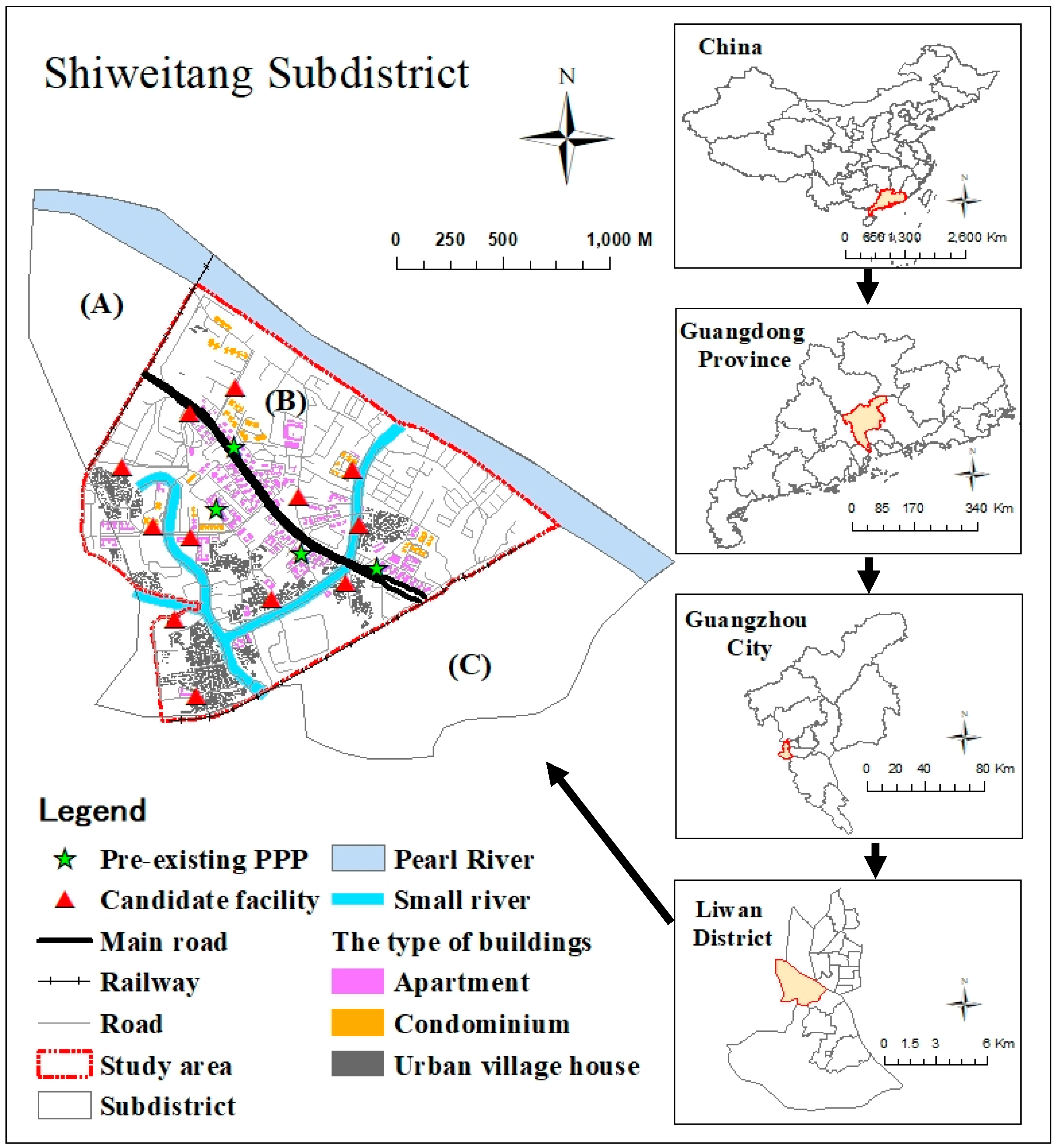
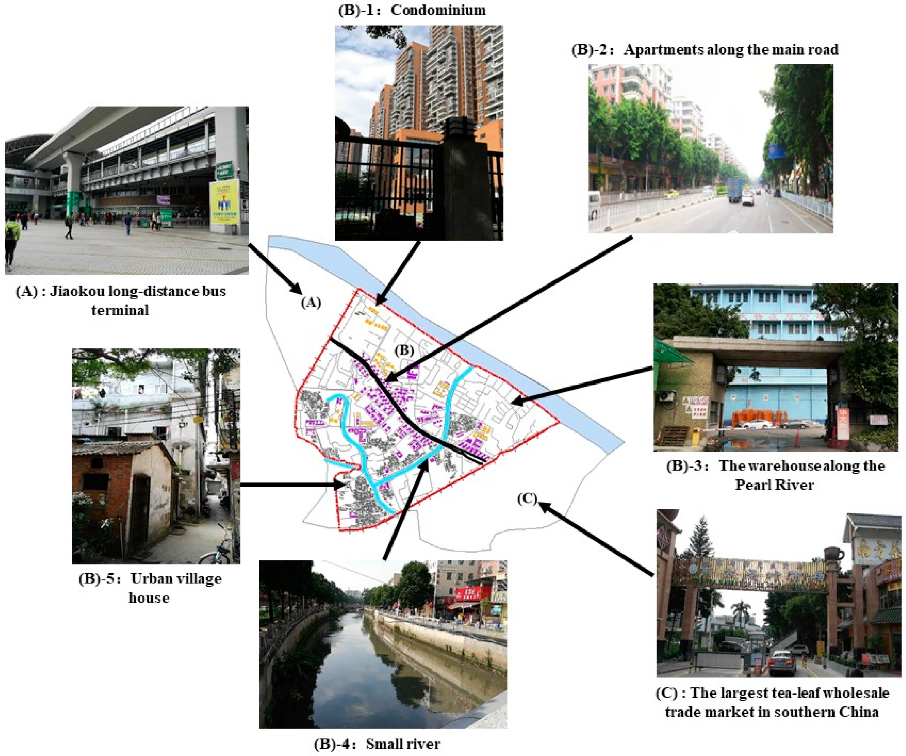
2.1. Study Area and Data
2.2. Methodology
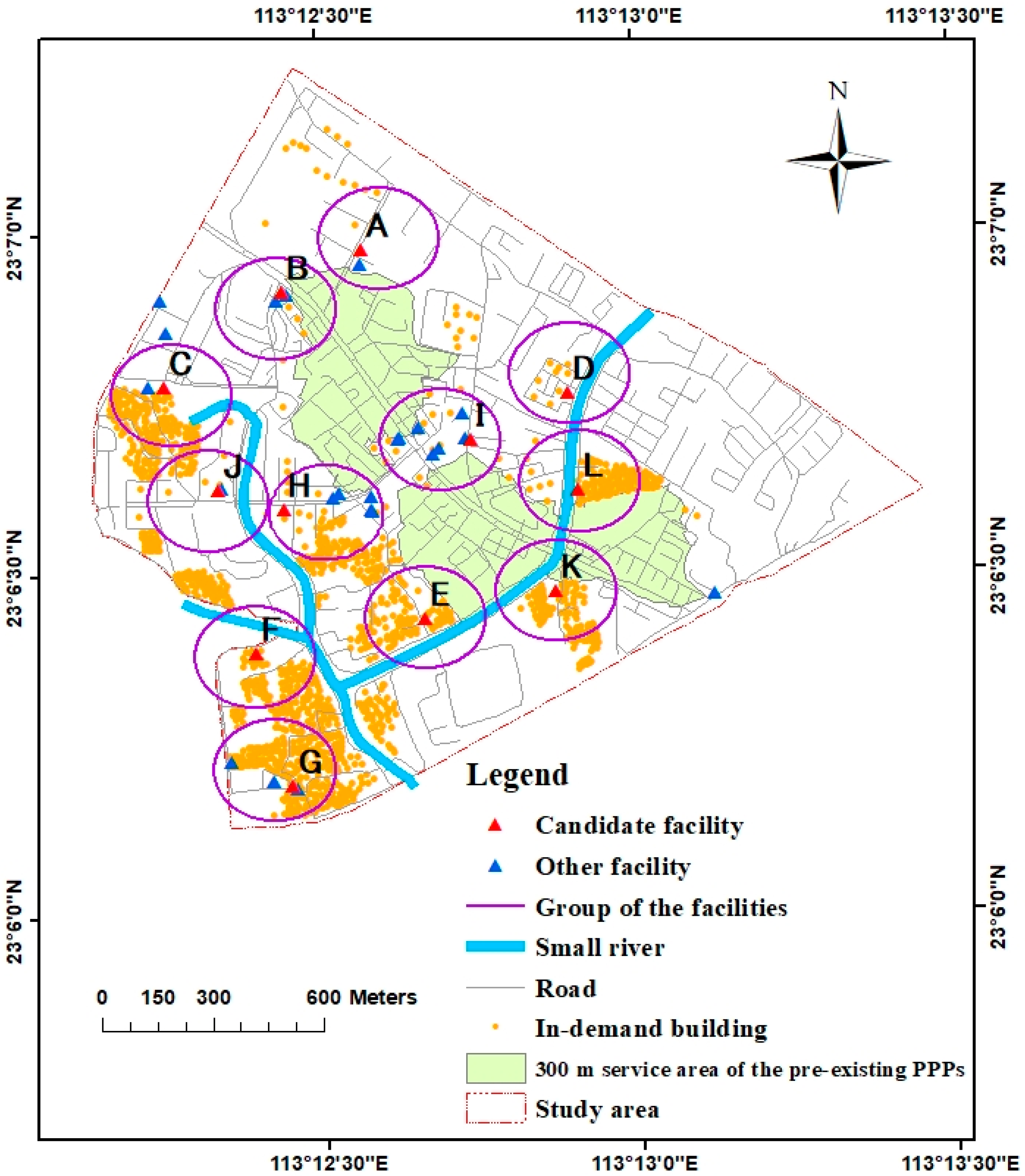
2.2.1. Defining Blank Service Areas and Candidate Facilities
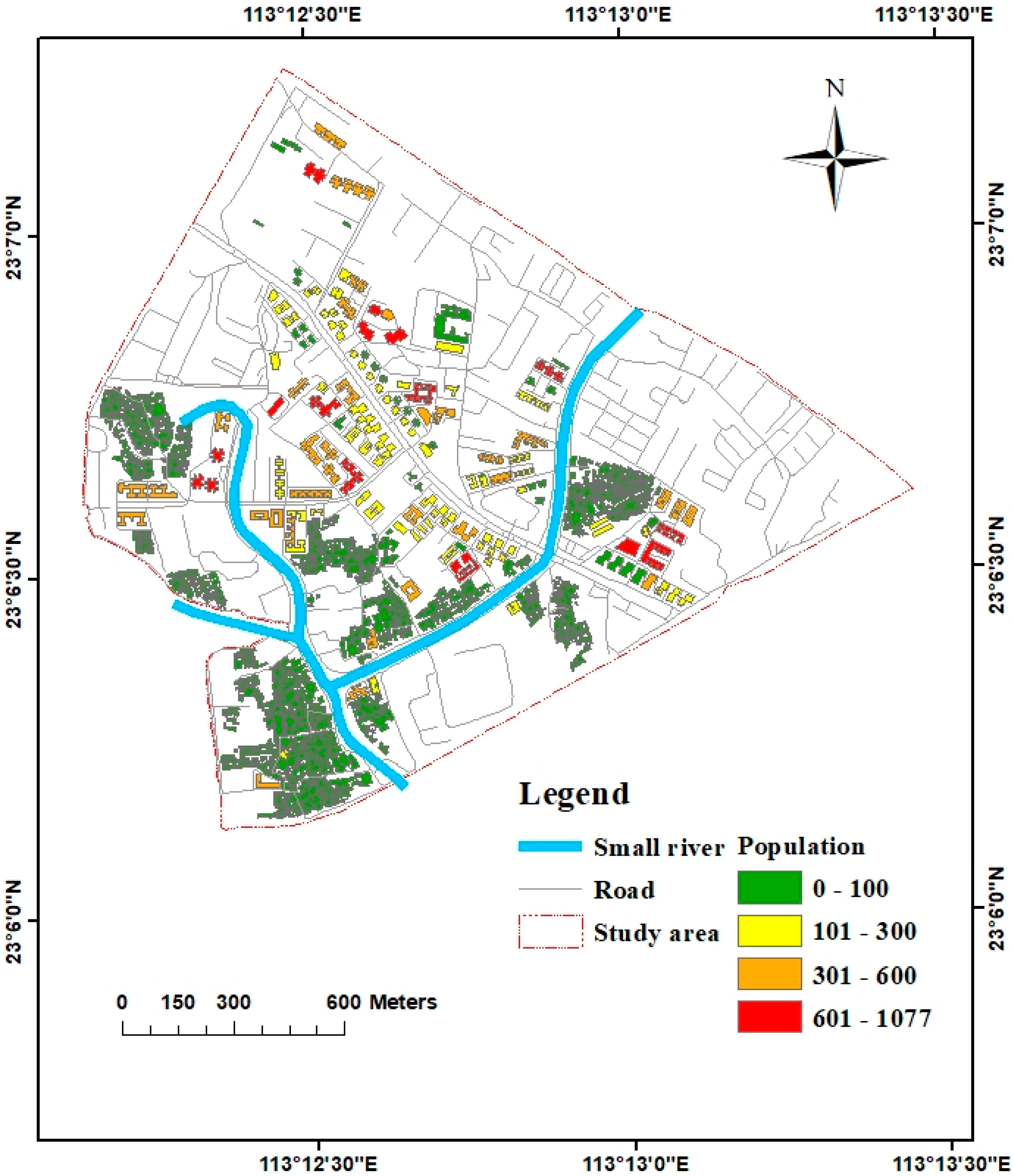
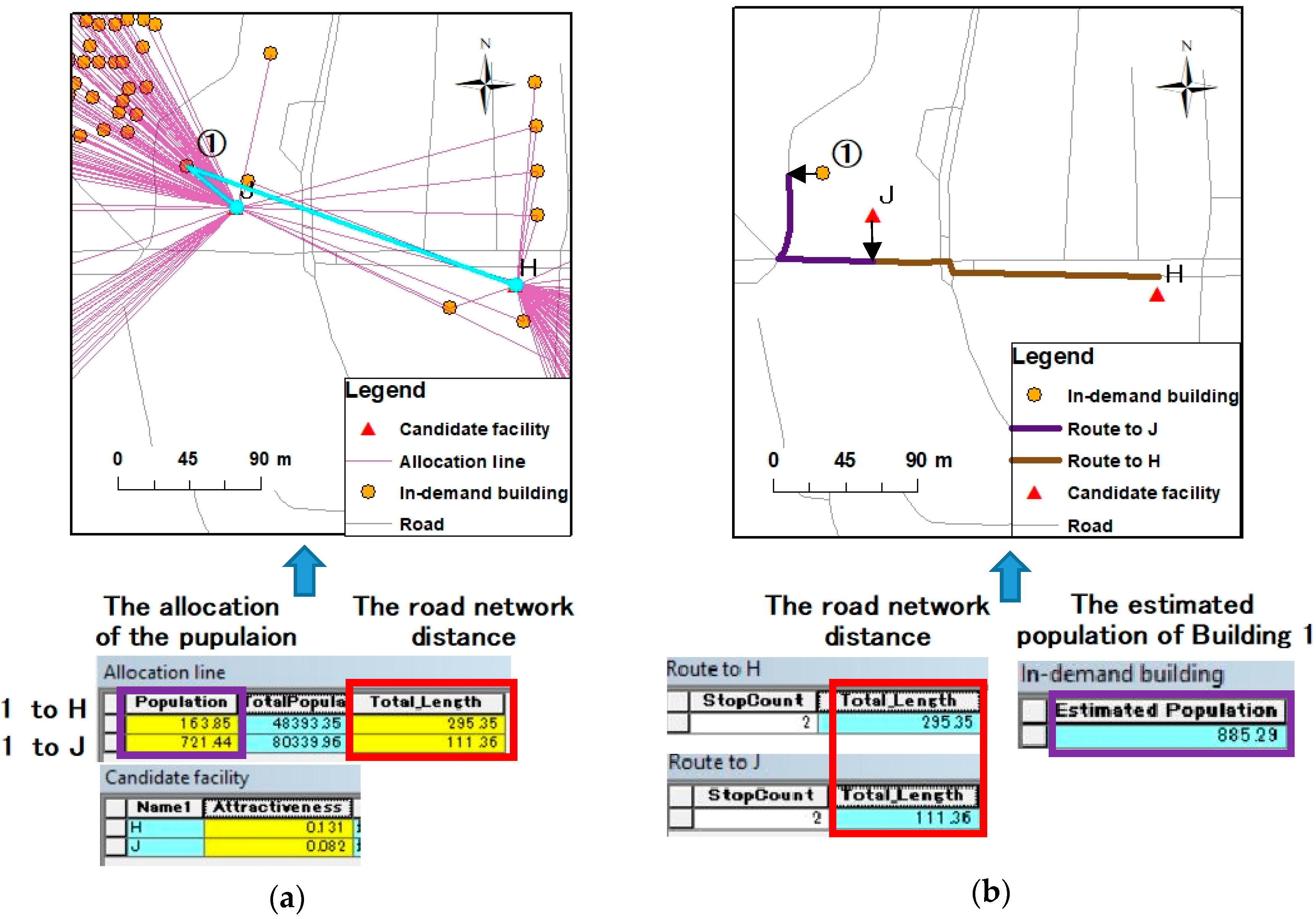
2.2.2. Estimating the Population of Residential Buildings
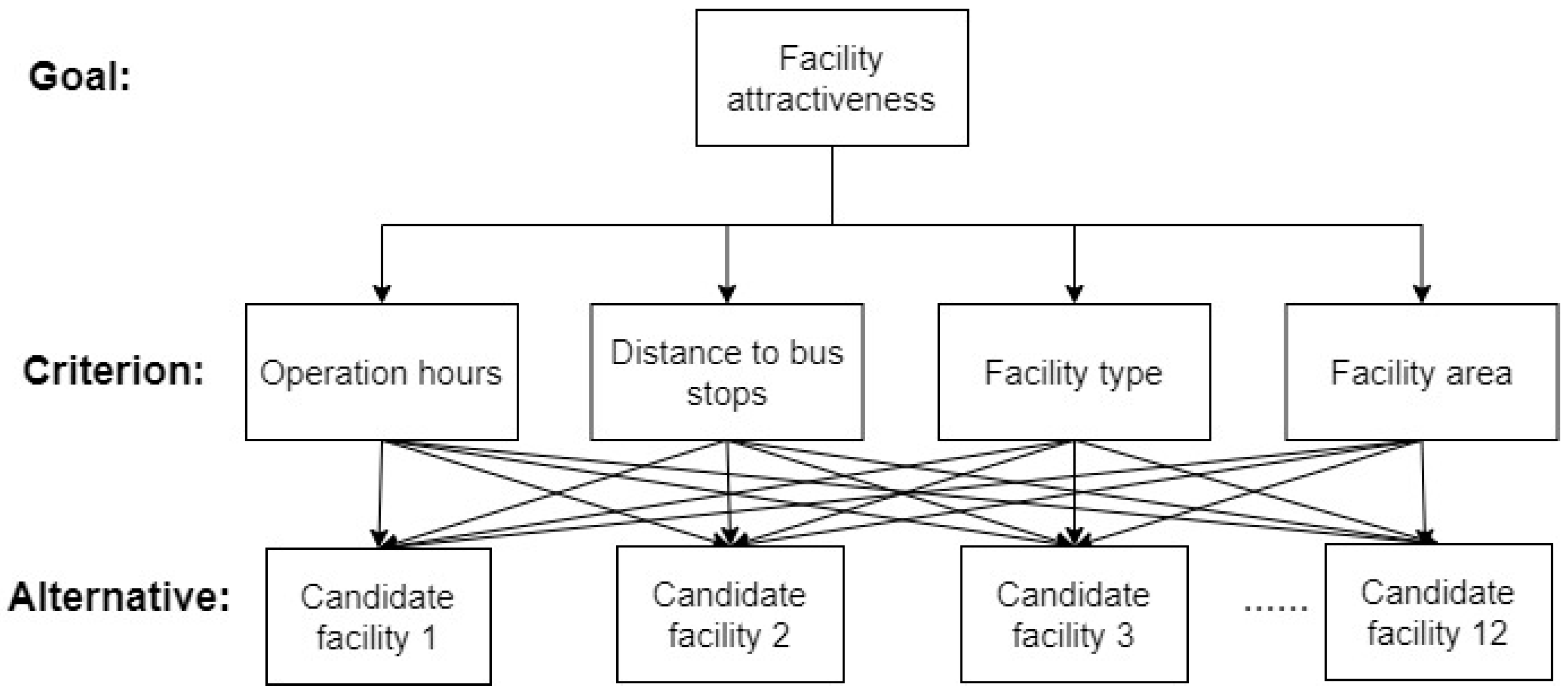
2.2.3. Calculating the Attractiveness of Different Alternative Facilities Using AHP
- Determining the criteria
- Building the AHP structure
- Computing the matrix of criteria weights and alternative weights
2.2.4. Estimating the Number of Customers of the Potential Facilities Using the Huff Model
3. Results
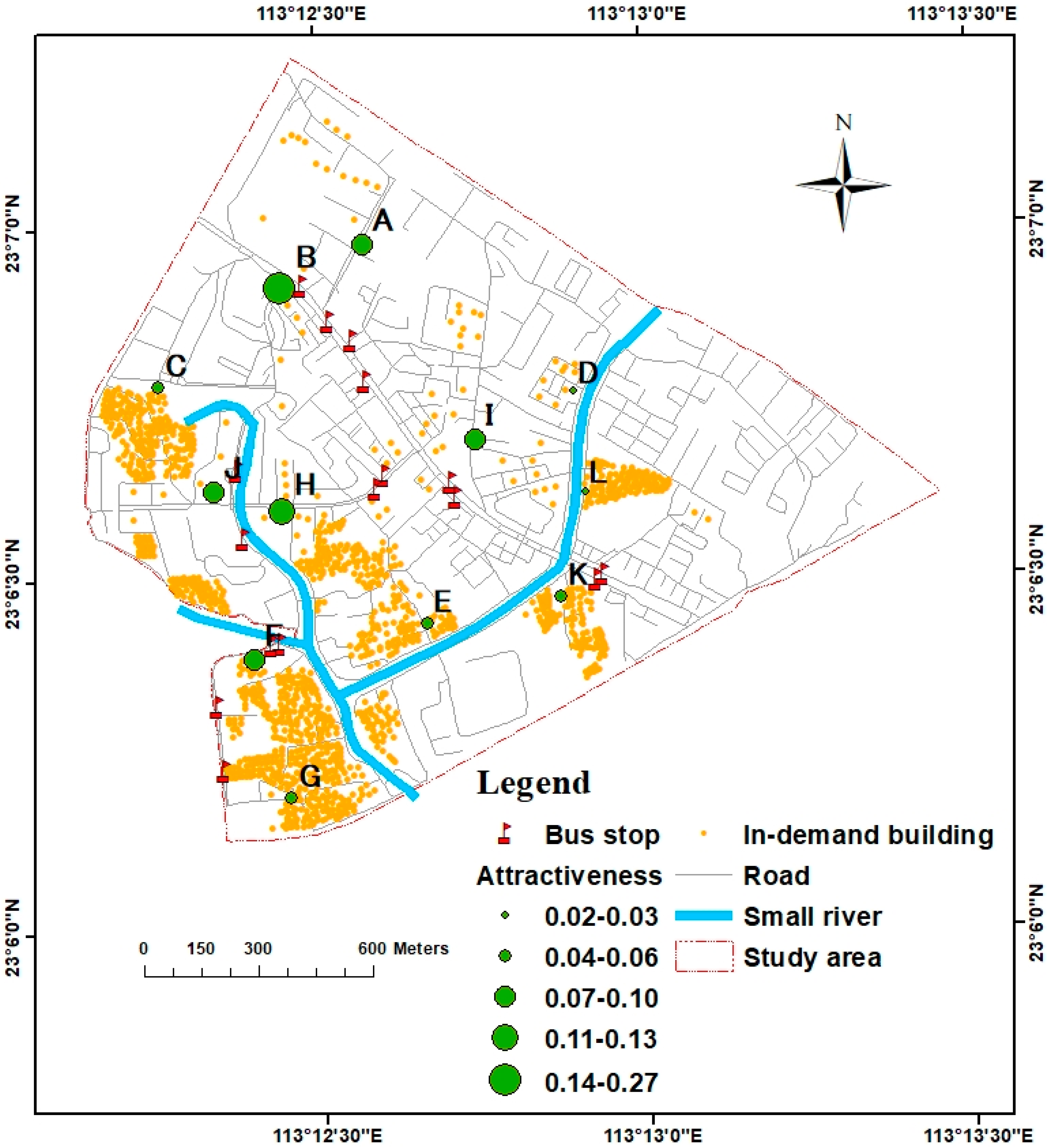
3.1. Criteria Weight and Facility Attractiveness
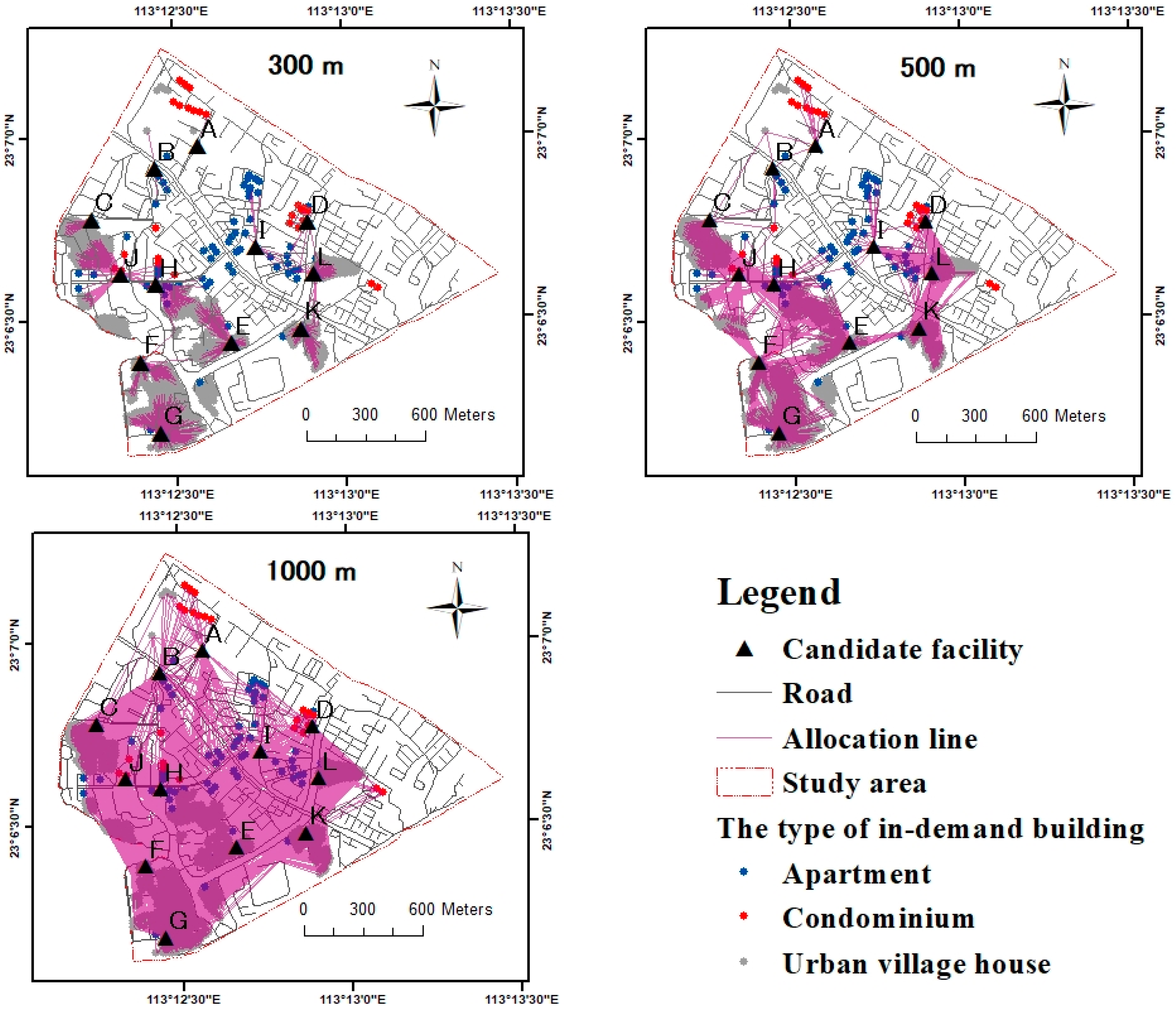
3.2. Optimal Facilities Based on the Huff Model
4. Discussion
4.1. Number of Potential Customers in the Facility’s Service Range is the Main Factor for the Optimal Facility
4.2. Effects of Acceptable Distance to the Facility Ranking
4.3. Accuracy of the Geographical Barrier Constraint Affects the Accuracy of the Model Results
4.4. Introduction of the AHP Method to Improve the Accuracy of Facility Attractiveness Value in the Huff Model
4.5. The Facility’s Attractiveness is More Sensitive to the Result of the Number of Customers in Case of a Long Acceptable Distance
5. Conclusions
Author Contributions
Funding
Acknowledgments
Conflicts of Interest
References
- Balcik, B.; Beamon, B.M.; Smilowitz, K. Last mile distribution in humanitarian relief. J. Intel. Transp. Syst. 2008, 12, 51–63. [Google Scholar] [CrossRef]
- Cárdenas, I.; Beckers, J.; Vanelslander, T. E-commerce last-mile in Belgium: Developing an external cost delivery index. Res. Transp. Bus. Manag. 2017, 24, 123–129. [Google Scholar] [CrossRef]
- Dablanc, L.; Liu, Z.; Combes, F.; Koning, M.; Coulombel, N.; Blanquart, C.; Heitz, A.; Klauenberg, J.; de Oliveira, L.K.; Seidel, S. CITYLAB Deliverable 2.1, Observatory of Strategic Developments Impacting Urban Logistics (2018 Version), Report for the European Commission 2018. Available online: http://www.citylab-project.eu/deliverables/D2_1.pdf (accessed on 23 February 2020).
- Edwards, J.B.; McKinnon, A.C.; Cullinane, S.L. Comparative analysis of the carbon footprints of conventional and online retailing: A “last mile” perspective. Int. J. Phys. Distrib. Logist. Manag. 2010, 40, 103–123. [Google Scholar] [CrossRef]
- Gevaers, R.; Van de Voorde, E.; Vanelslander, T. Characteristics and typology of last-mile logistics from an innovation perspective in an urban context. In City Distribution and Urban Freight Transport: Multiple Perspectives; Macharis, C., Melo, S., Eds.; Edward Elgar Publishing: Cheltenham, UK, 2011; pp. 56–71. [Google Scholar] [CrossRef]
- Gevaers, R.; Van de Voorde, E.; Vanelslander, T. Cost modelling and simulation of last-mile characteristics in an innovative B2C supply chain environment with implications on urban areas and cities. Procedia Soc. Behav. Sci. 2014, 125, 398–411. [Google Scholar] [CrossRef]
- Wong, C.Y.; Karia, N. Explaining the competitive advantage of logistics service providers: A resource-based view approach. Int. J. Prod. Econ. 2010, 128, 51–67. [Google Scholar] [CrossRef]
- Mokhtarian, P.L. A conceptual analysis of the transportation impacts of B2C e-commerce. Transportation 2004, 31, 257–284. [Google Scholar] [CrossRef]
- McKinnon, A.C.; Tallam, D. Unattended delivery to the home: An assessment of the security implications. Int. J. Retail Distrib. Manag. 2003, 31, 30–41. [Google Scholar] [CrossRef]
- Punakivi, M.; Yrjölä, H.; Holmström, J. Solving the last mile issue: Reception box or delivery box. Int. J. Phys. Distrib. Logist. Manag. 2001, 31, 427–439. [Google Scholar] [CrossRef]
- Junjie, X.; Min, W. Convenient pickup point in e-commerce logistics: A theoretical framework for motivations and strategies. Comput. Model. New Technol. 2013, 17, 209–213. [Google Scholar]
- Xiao, Z.; Wang, J.J.; Lenzer, J.; Sun, Y. Understanding the diversity of final delivery solutions for online retailing: A case of Shenzhen, China. Transp. Res. Procedia 2017, 25, 985–998. [Google Scholar] [CrossRef]
- Slabinac, M. Innovative solutions for a “Last-Mile” delivery—A European experience. In Proceedings of the 15th International Scientific Conference Business Logistics in Modern Management, Osijek, Croatia, 15 October 2015; pp. 111–130. [Google Scholar]
- Wang, J.J.; Xiao, Z. Co-evolution between etailing and parcel express industry and its geographical imprints: The case of China. J. Transp. Geogr. 2015, 46, 20–34. [Google Scholar] [CrossRef]
- Yuen, K.F.; Wang, X.; Ng, L.T.W.; Wong, Y.D. An investigation of customers’ intention to use self-collection services for last-mile delivery. Transp. Policy 2018, 66, 1–8. [Google Scholar] [CrossRef]
- Morganti, E.; Dablanc, L.; Fortin, F. Final deliveries for online shopping: The deployment of pickup point networks in urban and suburban areas. Res. Transp. Bus. Manag. 2014, 11, 23–31. [Google Scholar] [CrossRef]
- Collins, A.T. Behavioural Influences on the Environmental Impact of Collection/ delivery Points. In Green Logistics and Transportation; Springer: New York, NY, USA, 2015; pp. 15–34. [Google Scholar] [CrossRef]
- Roy, S.K.; Shekhar, V.; Lassar, W.M.; Chen, T. Customer engagement behaviors: The role of service convenience, fairness and quality. J. Retail. Consum. Serv. 2018, 44, 293–304. [Google Scholar] [CrossRef]
- Tan, R.; Xu, Y.; Chen, D.; Liu, L. Research on the spatial distribution of pickup points from the perspective of residents’ behavior. World Reg. Stud. 2016, 25, 111–120. [Google Scholar]
- Zhang, H.Y.; Shang, X. Analysis of express industry in the last mile distribution pattern—Taking as an example and rookie Inn Feng nest. Transp. Manag. World 2015, 22, 48–51. [Google Scholar]
- Church, R.L. Geographical information systems and location science. Comput. Oper. Res. 2002, 29, 541–562. [Google Scholar] [CrossRef]
- Hernandez, T. Enhancing retail location decision support: The development and application of geovisualization. J. Retail. Consum. Serv. 2007, 14, 249–258. [Google Scholar] [CrossRef]
- Joerin, F.; Thériault, M.; Musy, A. Using GIS and outranking multicriteria analysis for land-use suitability assessment. Int. J. Geogr. Inf. Sci. 2001, 15, 153–174. [Google Scholar] [CrossRef]
- Huff, D.L. Defining and estimating a trading area. J. Mark. 1964, 28, 34–38. [Google Scholar] [CrossRef]
- Huff, D.L. Parameter estimation in the Huff model. ESRI ArcUser 2003, October–December, 34–36. [Google Scholar]
- Suárez-Vega, R.; Santos-Peñate, D.R.; Dorta-González, P.; Rodríguez-Díaz, M. A multi-criteria GIS based procedure to solve a network competitive location problem. Appl. Geogr. 2011, 31, 282–291. [Google Scholar] [CrossRef]
- Coutinho-Rodrigues, J.; Simão, A.; Antunes, C.H. A GIS-based multicriteria spatial decision support system for planning urban infrastructures. Decis. Support Syst. 2011, 51, 720–726. [Google Scholar] [CrossRef]
- Kousalya, P.; Reddy, G.M.; Supraja, S.; Prasad, V.S. Analytical Hierarchy Process approach–An application of engineering education. Math. Aeterna 2012, 2, 861–878. [Google Scholar]
- Mckinsey Global Institute. China and the World. Available online: https://www.mckinsey.com/~/media/mckinsey/featured%20insights/china/china%20and%20the%20world%20inside%20the%20dynamics%20of%20a%20changing%20relationship/mgi-china-and-the-world-full-report-june-2019-vf.ashx (accessed on 23 February 2020).
- State Post Bureau of the People’s Republic of China. Statistical Communique on the Development of Postal Industry in 2018. Available online: http://www.spb.gov.cn/xw/dtxx_15079/201905/t20190510_1828821.html (accessed on 23 February 2020).
- State Post Bureau of the People’s Republic of China. Statistical Communique on the Development of Postal Industry in 2017. Available online: http://www.spb.gov.cn/xw/dtxx_15079/201806/t20180604_1581131.html (accessed on 23 February 2020).
- State Post Bureau of the People’s Republic of China. Statistical Communique on the Development of Postal industry in 2016. Available online: http://www.spb.gov.cn/xw/dtxx_15079/201705/t20170503_1150869.html (accessed on 23 February 2020).
- State Post Bureau of the People’s Republic of China. Statistical Communique on the Development of Postal Industry in 2015. Available online: http://www.spb.gov.cn/xw/dtxx_15079/201605/t20160510_757698.html (accessed on 23 February 2020).
- State Post Bureau of the People’s Republic of China. Statistical Communique on the Development of Postal Industry in 2014. Available online: http://www.spb.gov.cn/xw/dtxx_15079/201504/t20150429_462010.html (accessed on 23 February 2020).
- Guangzhou Statistics Bureau. Available online: http://tjj.gz.gov.cn/tjsj/index.html (accessed on 23 February 2020).
- Gaode Maps. Available online: https://ditu.amap.com/ (accessed on 23 February 2020).
- Lianjia Real Estate Agency. Available online: https://gz.lianjia.com/ (accessed on 23 February 2020).
- Wu, F.; Li, L.H.; Han, S.Y. Social sustainability and redevelopment of urban villages in China: A case study of Guangzhou. Sustainability 2018, 10, 2116. [Google Scholar] [CrossRef]
- Baidu Coordinate System. Available online: http://api.map.baidu.com/lbsapi/getpoint/index.html (accessed on 23 February 2020).
- Lwin, K.; Murayama, Y. A GIS approach to estimation of building population for micro-spatial analysis. Transact. GIS 2009, 13, 401–414. [Google Scholar] [CrossRef]
- Wind, Y.; Saaty, T.L. Marketing applications of the analytic hierarchy process. Manag. Sci. 1980, 26, 641–658. [Google Scholar] [CrossRef]
- Chuansheng, X.; Dapeng, D.; Shengping, H.; Xin, X.; Yingjie, C. Safety evaluation of smart grid based on AHP-entropy method. Syst. Eng. Procedia 2012, 4, 203–209. [Google Scholar] [CrossRef]
- Russo, R.; Camanho, R. Criteria in AHP: A systematic review of literature. Procedia Comput. Sci. 2015, 55, 1123–1132. [Google Scholar] [CrossRef]
- Masoud, R.G.; Farimah, M.R.; Maryam, G. Portfolio selection: A fuzzy-ANP approach. Financ. Innov. 2020, 6. [Google Scholar] [CrossRef]
- Saaty, T.L. Theory and Applications of the Analytic Network Process: Decision Making with Benefits, Opportunities, Costs, and Risks; RWS Publications: Pittsburgh, PA, USA, 2005. [Google Scholar]
- Goepel, K.D.; Performance, B. Comparison of judgment scales of the analytical hierarchy process—A New Approach. Int. J. Inf. Technol. Decis. Mak. 2019, 18, 445–463. [Google Scholar] [CrossRef]
- Simwanda, M.; Murayama, Y.; Ranagalage, M. Modeling the drivers of urban land use changes in Lusaka, Zambia using multi-criteria evaluation: An analytic network process approach. Land Use Policy 2020, 92, 104441. [Google Scholar] [CrossRef]
- Goepel, K.D. Implementation of an online software tool for the analytic hierarchy process (AHP-OS). Int. J. Anal. Hierarchy Process 2018, 10. [Google Scholar] [CrossRef]
- Harker, P.T. Incomplete pairwise comparisons in the analytic hierarchy process. Math. Model. 1987, 9, 837–848. [Google Scholar] [CrossRef]
- Oliva, G.; Setola, R.; Scala, A. Sparse and distributed analytic hierarchy process. Automatica 2017, 85, 211–220. [Google Scholar] [CrossRef]
- Pan, H.; Li, Y.; Dang, A. Application of network Huff model for commercial network planning at suburban–Taking Wujin district, Changzhou as a case. Ann. GIS 2013, 19, 131–141. [Google Scholar] [CrossRef]
- Dramowicz, E. Retail Trade Area Analysis Using the Huff Model. Dir. Mag. 2005. Available online: https://www.directionsmag.com/article/3207 (accessed on 23 February 2020).
- Derdouri, A.; Murayama, Y. Onshore wind farm suitability analysis using gis-based analytic hierarchy process: A case study of fukushima prefecture, Japan. Geoinfor Geostat: An Overv. 2018, S3. [Google Scholar] [CrossRef]


| Type | Data | Source | Format | Description |
|---|---|---|---|---|
| Spatial | Administrative boundary | National Geomatics Center of China (2017) | Vector (Polygon) | |
| Road | Ministry of Land and Resources of the People’s Republic of China (2015) | Vector (Line) | Updated by ArcMap software according to the Screenshot of Gaode maps Georeferencing | |
| Bus-stop | Vector (Point) | |||
| Building | Vector (Polygon) | |||
| Urban village area | Vector (Polygon) | |||
| Non-spatial | Population census | National Bureau of Statistics of China in 2010 |
| Factors | Percentage |
|---|---|
| Business hours | 99% |
| Distance to bus stops/subway station | 85 % |
| Facility type | 76 % |
| Facility area | 49% |
| Number of facility staff | 10% |
| Acceptable Distance | Percentage |
|---|---|
| 100 m | 15% |
| 300 m | 47% |
| 500 m | 34% |
| 1000 m | 4% |
| >1000 m | 0% |
| Ranking | Type of facility | Weight |
|---|---|---|
| 1 | Chain retail | 0.55 |
| 2 | Private retail | 0.29 |
| 3 | Chain service | 0.1 |
| 4 | Private service | 0.06 |
| Ranking | Criteria | Weight (Normalized) |
|---|---|---|
| 1 | Business time | 56.3% |
| 2 | Distance to bus stops/stations | 28% |
| 3 | Facility type | 11.2% |
| 4 | Facility area | 4.5% |
| Criteria | Business Time | Distance to Bus Stops/Stations | Facility Area | Facility Type | Overall Attractiveness |
|---|---|---|---|---|---|
| Weights | 56.30% | 28.00% | 4.50% | 11.20% | |
| Facility A | 0.072 | 0.043 | 0.071 | 0.162 | 0.074 |
| Facility B | 0.346 | 0.211 | 0.048 | 0.162 | 0.274 |
| Facility C | 0.069 | 0.019 | 0.018 | 0.034 | 0.049 |
| Facility D | 0.036 | 0.011 | 0.093 | 0.034 | 0.031 |
| Facility E | 0.072 | 0.015 | 0.048 | 0.034 | 0.051 |
| Facility F | 0.049 | 0.176 | 0.15 | 0.034 | 0.088 |
| Facility G | 0.072 | 0.05 | 0.018 | 0.034 | 0.059 |
| Facility H | 0.149 | 0.096 | 0.048 | 0.162 | 0.131 |
| Facility I | 0.072 | 0.084 | 0.309 | 0.162 | 0.096 |
| Facility J | 0.029 | 0.147 | 0.15 | 0.162 | 0.082 |
| Facility K | 0.019 | 0.114 | 0.033 | 0.012 | 0.045 |
| Facility L | 0.015 | 0.034 | 0.014 | 0.012 | 0.02 |
© 2020 by the authors. Licensee MDPI, Basel, Switzerland. This article is an open access article distributed under the terms and conditions of the Creative Commons Attribution (CC BY) license (http://creativecommons.org/licenses/by/4.0/).
Share and Cite
Zheng, Z.; Morimoto, T.; Murayama, Y. Optimal Location Analysis of Delivery Parcel-Pickup Points Using AHP and Network Huff Model: A Case Study of Shiweitang Sub-District in Guangzhou City, China. ISPRS Int. J. Geo-Inf. 2020, 9, 193. https://doi.org/10.3390/ijgi9040193
Zheng Z, Morimoto T, Murayama Y. Optimal Location Analysis of Delivery Parcel-Pickup Points Using AHP and Network Huff Model: A Case Study of Shiweitang Sub-District in Guangzhou City, China. ISPRS International Journal of Geo-Information. 2020; 9(4):193. https://doi.org/10.3390/ijgi9040193
Chicago/Turabian StyleZheng, Zilai, Takehiro Morimoto, and Yuji Murayama. 2020. "Optimal Location Analysis of Delivery Parcel-Pickup Points Using AHP and Network Huff Model: A Case Study of Shiweitang Sub-District in Guangzhou City, China" ISPRS International Journal of Geo-Information 9, no. 4: 193. https://doi.org/10.3390/ijgi9040193
APA StyleZheng, Z., Morimoto, T., & Murayama, Y. (2020). Optimal Location Analysis of Delivery Parcel-Pickup Points Using AHP and Network Huff Model: A Case Study of Shiweitang Sub-District in Guangzhou City, China. ISPRS International Journal of Geo-Information, 9(4), 193. https://doi.org/10.3390/ijgi9040193