Understanding Chinese Urban Form: The Universal Fractal Pattern of Street Networks over 298 Cities

Abstract

Urban form can be reflected by many city elements, such as streets. A street network serves as the backbone of a city and reflects a city’s physical structure. A street network’s topological measures and statistical distributions have been widely investigated in recent years, but previous studies have seldom characterized the heavy-tailed distribution of street connectivities from a fractal perspective. The long-tail distribution of street connectivities can be fractal under the new, third definition: a set or pattern is fractal if the scaling of far more small things than large ones recurs at least twice. The number of recurred scaling patterns of far more less-connected streets than well-connected ones greatly helps in measuring the scaling hierarchy of a street network. Moreover, it enables us to examine the potential fractality of urban street networks at the national scale. In this connection, the present study aims to contribute to urban morphology in China through the investigation of the ubiquity of fractal cities from the lens of street networks. To do this, we generate hundreds of thousands of natural streets from about 4.5 million street segments over 298 Chinese cities and adopted power-law detection as well as three fractal metrics that emerged from the third definition of fractal. The results show that almost all cities bear a fractal structure in terms of street connectivities. Furthermore, our multiple regression analysis suggests that the fractality of street networks is positively correlated with urban socioeconomic status and negatively correlated with energy consumption. Therefore, the fractal metrics can be a useful supplement to traditional street-network configuration measures such as street lengths.

1. Introduction

It is widely recognized that geographic features such as mountains and rivers are neither smooth nor regular, so they cannot be precisely described on the basis of Euclidean geometry. Instead, fractal geometry has the capacity to fill this gap. The very word “fractal” originates from Latin and literally means “broken” or “irregular”. The development of fractal geometry went through three definitions, all of which center on the term “self-similarity”: a part of an object or pattern is similar to the whole [1,2,3]. For the first and second definitions, fractals refer to shapes that are either strictly or statistically self-similar. A classic example of strictly self-similar shapes is a Koch curve [4], whose parts are exactly the scaled copies of the original curve. Mandelbrot [5] relaxed the strictness by adding some randomness to those “scaled copies” to make the constructed curve capable of describing real-world features, such as a coastline. Strict and statistical self-similarities both maintain the same power law exponent or the fractal dimension from the power law relationship between the number of copies in the fractal and the scale at which it is measured. As the power law relationship is too tough to universally see the real-world fractals, Jiang and Yin [6] further relaxed this statistical requirement by checking if the pattern of scaling—far more small scales than large ones—of a fractal recurs at least twice. In the third definition, the focus of self-similarity is no longer on the geometric form, but rather on the recurring pattern of scaling statistics among iteratively derived sub-wholes of data.

Urban space exhibits fractal patterns from two main perspectives. Morphologically, a large body of literature presents the fractal evidence from many urban elements—for instance, built-up areas, land uses, streets, and boundary shapes [7,8,9,10,11,12], and their evolution or growth (e.g., [13,14,15]). Functionally, human activities inside an urban space, especially those manifested by location-based social media data, agglomerate into a fractal-like structure that contains a minority of high-density locations and a majority of low-density ones, which are ordered spatially from the city center to the periphery [16,17]. Such spatial configuration of human activities is also claimed to be akin to the fractal structure of central place systems [18]. Among those aforementioned city elements, urban streets are most broadly adopted for understanding both a city’s form and function. On one hand, streets represent a city’s physical environment and showcase the coherency of its spatial organization. On the other hand, human urban activities or movements are, to a large degree, confined within the network of streets. Therefore, it is important to examine fractal cities from the perspective of street networks in order to obtain new insights into a city’s underlying spatial environment, its configuration, and the human activities therein.

As one particular type of complex networks whose nodes and links are located in the geographic space, street networks are naturally modeled as graph representations, wherein the dual graph (nodes as streets, links as intersections; [19]) enable us to analyze the street structural configuration through a set of topological measures based on graph theory [20,21] and space syntax approaches [22]. Similar to many other real-world complex networks, such as social networks and protein interactions, the dual graph of street networks tend to possess a fractal or scaling property with respect to the power law distribution of the node degrees [20,23], or the power law relationship between the number of non-overlapping compartments covering the entire network and their sizes [24,25,26]. However, because the power law model is too strict to measure a fractal whose statistical distribution follows a non-power-law but still appears to have fat-tailed characteristics (e.g., log-normal), the assessment of whether street networks are fractals across a large variety of cities is challenging. Then, this paper is motivated to use the third definition of fractal, which unties the power law constraint by considering other types of heavy-tailed distribution as the support of fractality, to identify the universal fractal pattern of street networks at a wide spatial extent.

Another triggering factor of this research is the geospatial big data. The limited data availability and computational resources in the past has led to a relatively narrow spatial scope of works belonging to urban street networks; that is, a neighborhood or city level [27]. Big data offers unprecedented opportunities for researchers to achieve the massive-scale geospatial data sets. For example, through OpenStreetMap (OSM), a volunteered geospatial information platform, we are able to achieve and process the street network nationwide, or even worldwide coverage, which creates new opportunities to investigate street fractalities at intercity levels within a country or across countries [28]. Not only can the national road network be accessed, but other national urban quantities can be easily accessed as well, such as Gross Domestic Product (GDP) and CO₂ emissions. This opens the possibility for us to unpack the relationship between street-network configuration and urban energy, environmental, and economic indicators. Prior urban-scale studies have reported that streets with fractal features can contribute to the enhancement of social capital and the reduction of greenhouse gas emissions because of larger street-network efficiency (e.g., [26,29]). This study would conduct such exploratory analysis on the country scale.

The contribution of this study is three-fold. Firstly, we employed the natural street representation (a continuous street rather than its contained meaningless segments or vertices; see the details in Section 2.2) for the identification of the fractal or scaling structure. We have successfully processed and derived the natural streets for almost all prefectural-level cities in China, which could be a valuable data source for the research community. Second, we designed an innovative methodology in combining different fractal metrics under the theoretical framework of the third definition. Starting from the head/tail breaks-induced ht-index [6], we can assess the fractality of the street network for each individual city and the overall complexity of all street networks at a country scale. Next, due to the lack of sensitivity of the ht-index, we employed two alternatives: the cumulative rate of growth (CRG, [30]) and the ratio of areas in a rank-size plot (RA, [31]) (see more details in Section 2.3). We found that using them collectively can differentiate cities within the same scaling hierarchy, making it possible to formulate a more comprehensive and systematic understanding of Chinese urban forms. Lastly, we sought relationships between the fractality of street networks and different kinds of urban metrics and evaluated the explanatory power of urban fractals on urban socioeconomic status and energy consumption at the national scale.

The remainder of this paper proceeds as follows. Section 2 introduces the data sets and the proposed methodological framework. Section 3 presents the visualization and statistical results regarding the universal fractal pattern over nearly 300 cities in China, as well as the correlations between each fractal metric and urban quantity. Section 4 further discusses the fractal structure of street networks, before Section 5 draws conclusions and points to future research directions.

2. Data and Methods

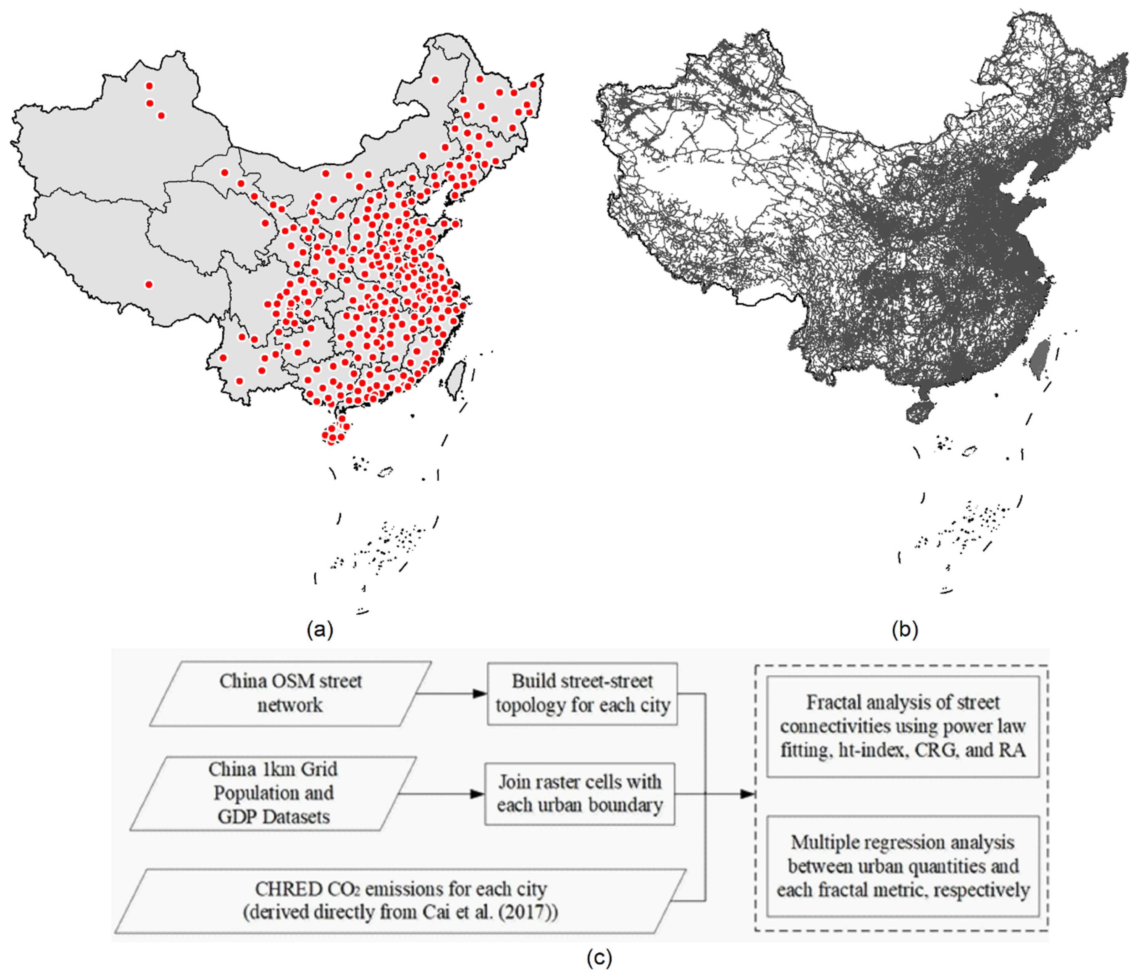
2.1. Data and Data Processing

Three data sets were used in this study: (1) 298 city boundaries, (2) the national street network, and (3) China grid data sets of GDP, population, and CO₂ emissions. As illustrated in Figure 1, we selected 298 prefectural-level cities that were spread all over China as the study areas. Each city boundary is further adopted as the unit for data processing. The national street network was downloaded from a Germany free Geodata platform GEOFABRIK [32]. We used ArcGIS Interoperability Toolbox to process the large collection of polylines with all road types into 4,419,603 segments to ensure that each segment’s end vertex is the street junction where at least three polylines intersect, and then we clipped the entire set of segments using each urban boundary to obtain the city-level streets. The national GDP and population grid data were sourced from the National Resources and Environment Database of the Chinese Academy of Sciences [33]. The data were collected in 2015 and spatialized by remote sensing technology with a ground resolution of 1 km (for more details of this approach, see [34]). City-level GDP and population statistics were calculated successfully by aggregating the cell values within each city boundary. The city-level CO₂ emissions were derived directly from the previous work [35], which provides related statistics based on CHRED (China high-resolution emission database; see more details in [36]). Note that the urban-scale CO₂ emissions in Cai et al.’s [35] work are only available for 283 cities.

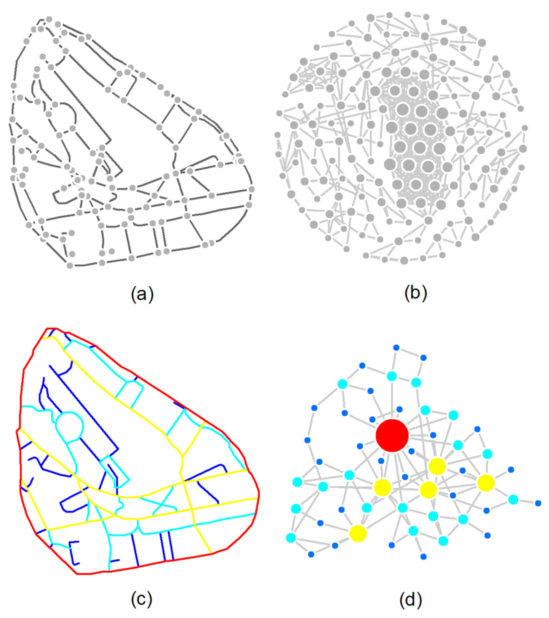
2.2. Transformation from Segment–Segment Topology to Street–Street Topology

Segment–segment topology is widely adopted in current GIS systems. For example, the ArcGIS Network Analyst extension builds up the network analysis based on the relationship between segments that are separated at a street junction node. The segment–segment topology, or segment-based analysis in general, is remarkable because it offers many urban applications, such as navigation. However, the segment–segment topology is essentially a geometric perspective because the modeling unit of the street network is based on geometric primitives, such as points, polylines, and polygons. The geometric primitives represent space mechanically, as their lengths or connectivities tend to follow a normal-like distribution (Figure 2a,b).

In order to view the space more organically, one can consider transforming the segment–segment topology into the street–street topology. A street refers to the notion of a “natural street” or “named street”, which is made up of a set of neighboring segments with good continuity or shared names [37]. The good continuity can be understood as small deflection angles (that is, those smaller than 45 degrees) across adjacent segment pairs. Compared to segments, streets such as the modeling unit are coherent and meaningful in our perception [22]. Moreover, the street–street topology allows us to investigate the street network from a complex-network perspective [38], as the street lengths and connectivities under such a setting tend to be scale-free or heterogeneous, indicating far more short/less-connected streets than long/well-connected ones (Figure 2d). Although it is possible that street length correlates with street connectivity, we have only used street connectivity for the following experiments because individual street length is not a major factor for understanding the urban space. This can be easily understood by the fact that a well-connected street is commonly found in a city, whereas a long street is often not a well-connected street and is usually found in the countryside.

2.3. Fractal Analysis of Street Connectivities

The fractal structure of urban street networks can be characterized by power law or other heavy-tailed distribution models regarding the street connectivities. As the power law model may be too strict to identify a fractal, we derive the scaling hierarchies of streets using head/tail breaks [39] and compute three metrics—the ht-index, CRG, and RA—to measure the potential fractality of the street network.

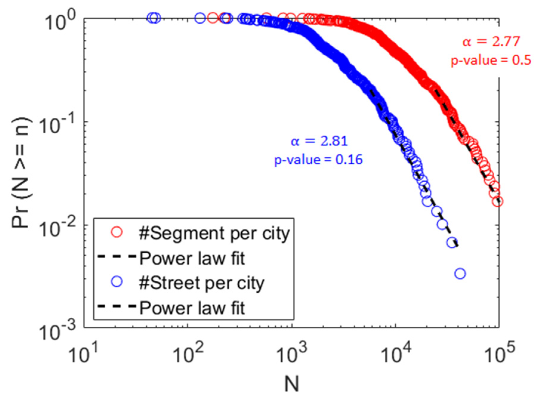
2.3.1. Power Law Detection

A power law model can be expressed by Equation (1):

$$y=x^{-\alpha }.$$

(1)

The simplest way to identify a power law distribution is by ranking the data values from largest to smallest and then creating a log-log plot of the sorted data. The distribution will be a straight line if the data exactly follows a power-law distribution. However, it is very difficult for this method to deal with the messy up-and-downs in the tail for many real-world data sets [40]. To address this problem, a robust method using maximum likelihood estimation, proposed by Clauset et al. [41], can help detect accurately whether data is a power law or not. The method firstly examines the power law exponent $\mathsf{\alpha }$, which is denoted by Equation (2):

$$\mathsf{\alpha }=1+\mathrm{n}{\left[{\displaystyle \sum }_{i=1}^n\ln \frac{x_i}{x_{min}}\right]}^{-1}$$

(2)

where $x_{min}$ is the smallest value from where the data is power-law distributed. The acceptable range for exponent $\mathsf{\alpha }$ is from 1 to 3. To test how good the data can fit with a power law, Clauset et al. [41] suggest doing a Kolmogorov–Smirnoff test. This test compares the data with the samples based on an ideal power law distribution, using the derived x-min and alpha values. The goodness-of-fit index p-value, ranging from 0 to 1, is then generated and used to determine the extent of fitness for the data to a power law model. If p-value $\ge$ 0.01, we accept a set of data being power-law distributed.

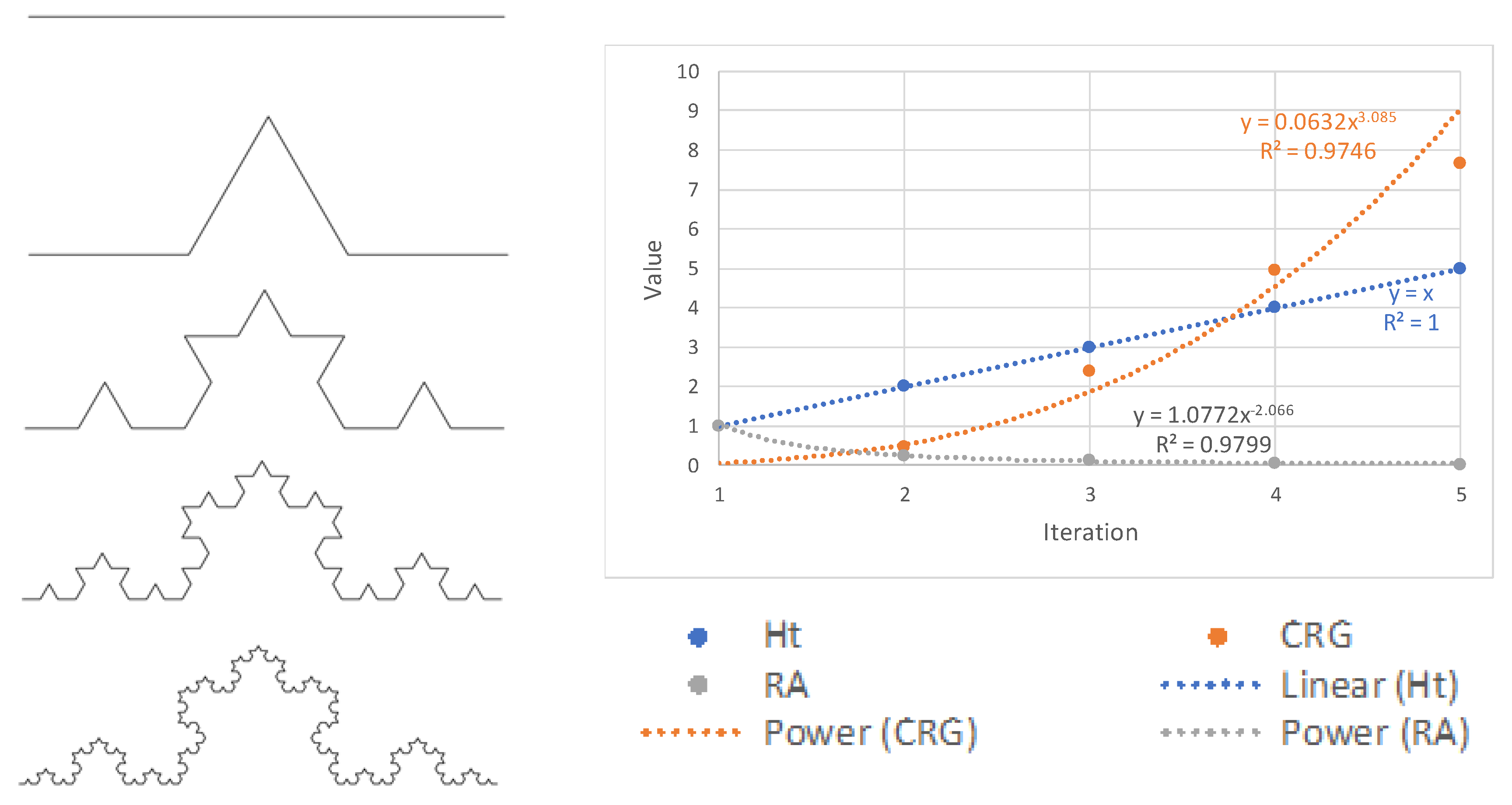
2.3.2. Integration of Ht-Index, CRG, and RA for Fractal Measurement

Jiang and Yin [6] proposed the third definition of fractal as “the recurrence of far more smalls than larges” and induced a new metric ht-index, coming from the new classification scheme head/tail breaks [39]. To elaborate, given data with a heavy-tailed distribution, we can always split the data into a great many small values (that is, the tail) and a few large values (the head). Note that there is an imbalance between head percentage and tail percentage (for example, 40/60). The splitting operation is called head/tail division. We can apply this division iteratively to the head part of the data until the updated head and tail percentages reach a balance, such as 50/50. The entire process demonstrates how the head/tail breaks method [39] works. Since the process is recursive, we would normally achieve a series of mean values. The number of obtained mean values $i$ plus one is the so-called ht-index, as expressed by Equation (3):

$$\mathrm{ht}=i+1$$

(3)

Figure 3a shows the first three iterations of a Koch curve [4]. The first iteration contains one segment with a scale of 1; the second contains four segments with a scale of 1/3; the third contains 16 segments with a scale of 1/9. The fractal dimension, i.e., the power law exponent between its details and scales, equals to the slope of log-log plot as shown in Figure 3b. To apply the head/tail breaks method, we rank all scales of the Koch curve from the largest to the smallest (a rank-size plot, Figure 3c). The induced ht-index value of the Koch curve is 3, meaning that the scaling pattern of far more short segments than long ones appears twice. Two mean values were computed: m₁$=\frac{16\ast \frac{1}{9}+4\ast \frac{1}{3}+1\ast 1}{21} \approx$ 0.195 and m₂$=\frac{4\ast \frac{1}{3}+1\ast 1}{5}$ $\approx$ 0.46. In this way, we can derive the curve’s three scaling hierarchical levels: 16 segments whose scales are below m₂, four segments whose scales are between m₁ and m₂, and one segment whose scale is above m_1. The proposal of the ht-index is significant in many aspects of computing the fractality of a geographic feature. The ht-index extends the usage of other heavy-tailed distribution mathematic models to quantify a fractal. Furthermore, as the fractal dimension does not focus on the change of scales among different iteration stages, the ht-index supplements the fractal dimension in terms of measuring the growth of a fractal as the iteration goes. However, the ht-index suffers from distinguishing two fractals with slightly different patterns but the same ht-index value, as the ht-index value is formatted as an integer. To solve the insensitivity of the ht-index, several fractal metrics have been developed, such as CRG and RA [30,31].

CRG is calculated by adding the ratios between consecutive mean values, which is expressed by Equation (4):

$$\mathrm{CRG}= \{\begin{array}{cc}0,\hfill & \hfill i=0\\ m_{1, }\hfill & \hfill i=1\\ {{\displaystyle \sum }}^{}\frac{m_{i+1}}{m_i},\hspace{1em}\hfill & \hfill i>1\end{array}$$

(4)

where $i$ denotes the i_th mean values during the head/tail breaks process. Taking the Koch curve in Figure 3a again as a working example, its CRG equals m₂ /m₁ = 0.46/0.2 = 2.38, which supports decimal values, so that the CRG can capture the growth of a fractal more sensitively.

RA is an index that examines the extent to which the numeric values are long-tail distributed. To compute RA, we can obtain the ratio between the areas of two polygons A and B based on the rank-size distribution (Figure 3d), as denoted by Equation (5).

$$\mathrm{RA}=\frac{S_A}{S_A+S_B}$$

(5)

where $S$ is the area of a polygon formed by the distribution line.

In sum, it can be said that the ht-index is the primary metric responsible for the fractal characterization. The CRG and RA indices were, to a large extent, the alternatives to the ht-index, and their major advantage is capturing the sensitivity that the ht-index cannot. More specifically, the CRG sums the differences between every two consecutive hierarchical levels, while RA summarizes the overall distance of the whole population from a heavy-tailed distribution to a normal distribution. Here, we add two more iterations of a Koch curve for clearer illustration. As

Table 1. The three metrics under the new fractal definition at each iteration of the Koch curve.

Iteration	Ht	CRG	RA
1	1	0	1
2	2	0.46	0.25
3	3	2.38	0.14
4	4	4.95	0.07
5	5	7.65	0.03

and Figure 4 show, CRG and RA changes nonlinearly as the iteration goes, while the ht-index values appear to be linear. It is also interesting to find that CRG and RA are complementary to each other. Since CRG is an upward trend whose range is [0, $\infty )$ (the higher the CRG, the more scaling hierarchical levels the data), while RA is downward from 1 to 0 (the lower the RA, the more heavy-tailed distributed the data). Together with CRG and RA, we can differentiate fractals with the same scaling hierarchy or the same ht-index value. However, at present, these three metrics are rarely combined for a more comprehensive understanding of a fractal. In this study, we integrate the ht-index, CRG, and RA to implement the fractal analysis of street connectivities for each urban street network.

2.4. Regression Analysis

Prior studies have assessed the growth of the Chinese prefectural-level city system using urban quantities; for example, GDP and population [42]. This study inspects the linkage between Chinese urban quantities and street structure with the identified fractal pattern. To do this, we conduct a multiple regression analysis to unpack relationships between fractal metrics and collected urban indicators including socioeconomic factors (GDP and population) and carbon emissions. Apart from three fractal metrics, we follow the previous study [43] by introducing the city area, number of streets (#Streets), and total length of streets ($l_{\forall Streets}$) as variables to the regression model to estimate comprehensively the explanatory power of street-network configuration measures on cities’ socioeconomic status. We take the logarithm of some metrics to scale all variables in a similar magnitude. Therefore, the multiple regression model takes the following form as Equation (6) denotes:

$$\log \left(GDP\right)={\beta }_0+{\beta }_1\ast \log \left(Area\right)+ {\beta }_2\ast \log \left(\#Streets\right)+ {\beta }_3\ast \log \left(l_{\forall Streets}\right)+{\beta }_4\ast ht+{\beta }_5\ast CRG+{\beta }_6\ast RA.$$

(6)

We also run two multiple regression models respectively with log(population) and log(CO₂ emissions) as the dependent variable. The correlation analysis was conducted based on the Regression tool in Microsoft Excel software.

3. Results and Discussion

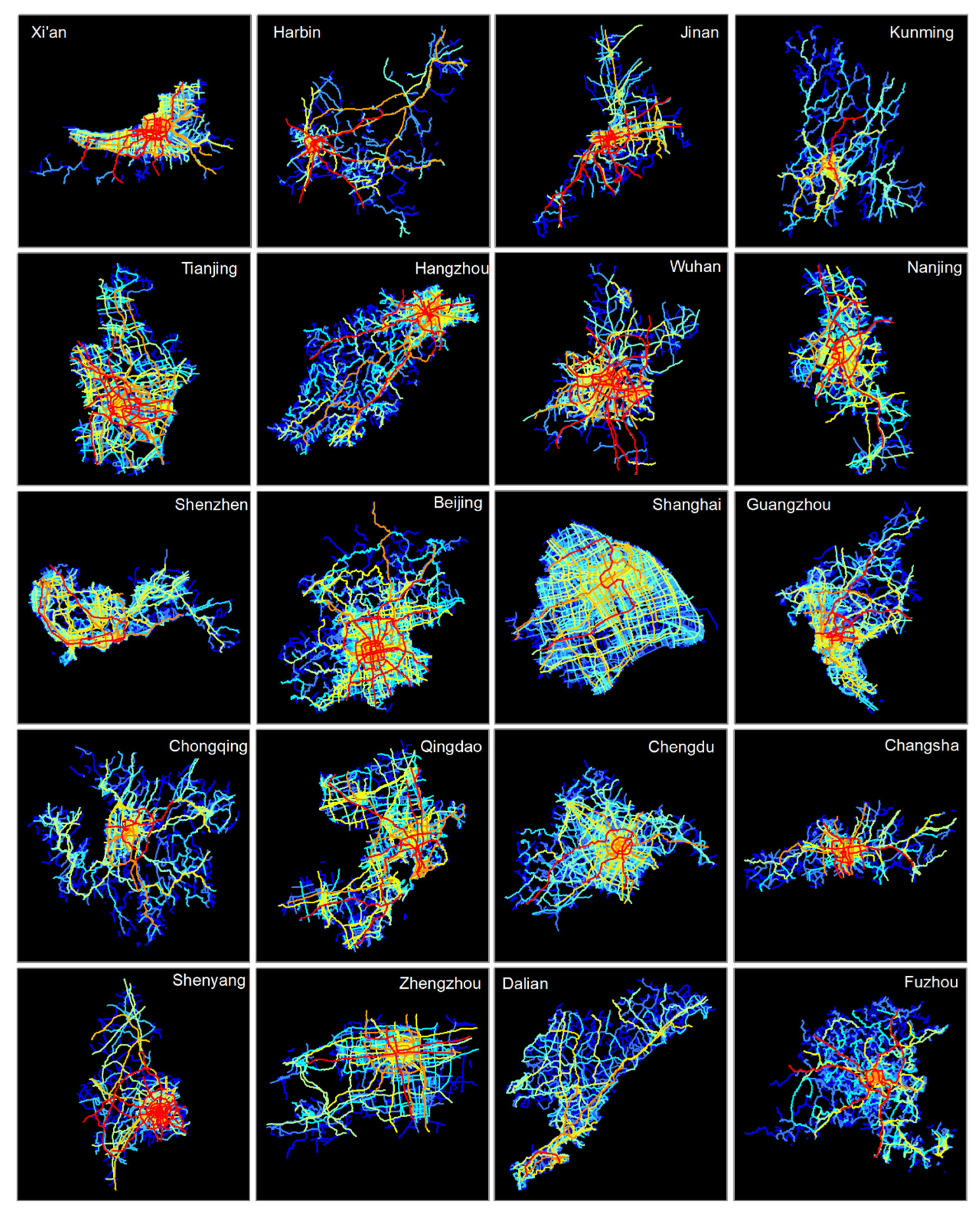
3.1. The Universal Fractal Pattern of 298 Urban Street Networks

The natural streets were generated for all urban street networks; the number of segments and the number of streets ranged from 173,360 and 34,924 (Shanghai) to 175 and 49 (Wuzhishan). The number of segments and the number of streets for each city both obey the power-law distribution (Figure 5). The number of resulting streets for each city on average is 4.4 times smaller than the number of segments. We applied the head/tail breaks method on the number of streets for all cities and produced an ht-index of 4. From

Table 2. Head/tail breaks statistics for the number of natural streets for 298 cities.

#City	#Head	%Head	#Tail	%Tail	Avg #Streets
298	83	27%	215	73%	3923
83	27	32%	56	68%	9506
27	9	33%	18	67%	16464

, we noted that each head percentage was very low (around 30%). This indicates that only a minority of cities possess more than 10,000 streets and most cities have 4000 or fewer streets, given the data sets provided by OSM.

Next, we computed the ht-indexes in terms of street connectivities for each city. Almost all cities had an ht-index value greater than or equal to 3, except for one city (Wuzhishan) whose ht-index value was only 1. The top four cities in terms of ht-index are Shanghai, Dongguan, Hangzhou, and Jinhua, all of which are cities located in highly developed areas of China (for example, around the Yangtze River Delta). Most of the important cities, such as municipalities directly under the central government and provincial capital cities, possess ht-indexes above 5. We can see from

Table 3. Ht-indexes of street connectivities for 298 cities. (Note: the number in brackets indicates the number of cities whose street connectivities pass the power-law test).

Ht-index	1	3	4	5	6	7	8	9
#City	1 (0)	7 (4)	44 (32)	78 (48)	81 (52)	62 (43)	21 (16)	4 (4)

that more than 80% of cities have ht-indexes above 4, indicating that in each of those cities, the scaling pattern of far more less-connected streets than well-connected ones recurs at least four times. These underlying scaling hierarchical levels at the city scale help us identify the ubiquity of fractal patterns of Chinese urban street networks. We also conducted the power-law detection for the degree of connectivity of each urban street network. In total, there are 199 cities whose street connectivities pass the power-law test. We took a closer look at cities with the same street hierarchical level (that is, the same ht-index value) and found an obvious trend that street networks with a higher ht-index value tend to pass the strict power law examination, as the percentage of “power-law-distributed cities” generally grows when the ht-index increases (Table 3).

To investigate the urban street networks more precisely, we further calculated the CRG and RA indexes for each city. For visualization purposes, we normalized both CRG and RA within the range [0, 1], and used 1 – RA to show the results in order to keep the CRG and RA values in the same direction; that is, the more upper right, the more fractal the city (Figure 5). Specifically, we can say that the x-axis represents the increment of summed differences of every two consecutive hierarchical levels, while the y-axis shows the closeness of a power-law distribution.

The plot can be explained from both global and local perspectives (Figure 6 and Figure 7, respectively). Globally, the distribution of cities using CRG and RA largely follows the distribution using the ht-index. However, because of the great increase of sensitivity, the differences between cities within the same or across different ht-indexes can be effectively detected. For example, Shanghai, which has both the largest CRG and 1 – RA, was the most fractal city among the top four cities with an ht-index of 9; Beijing, with an ht-index of 7 but a perfect power-law (alpha = 0.58, p-value = 0.26, and 1 – RA = 1), resided uppermost and, more interestingly, in the middle of cities whose ht-indexes were 8.

Locally, we can spot that CRG and RA correlated very well at each ht-index, as the cities with the same ht-index value clustered and distributed around the trend line (Figure 6). For instance, the correlation between CRG and RA can be best depicted using a second-order polynomial function when the ht-index = 5, 6, and 7 (Figure 7b–d), while the CRG linearly correlates with RA when the ht-index = 8 (Figure 7a). The good correlation indicates the positive relationship between the summed differences among hierarchical levels and the nearness of being a power law. As the CRG and RA are not 100% correlated, the trend line, in this connection, works as a “ruler” to discriminate what matters more in a fractal pattern: being more power law (above the trend line) or having more growth between its hierarchical levels (below the trend line). From Figure 7, we found one thing in common for each correlation plot: in most cases, cities with higher economic (based on derived urban GDP) or political status (if a provincial capital city or city under central government) are located at the more upper-right part of the figure area or above the trend line. This implies that the degree of connectivity in street networks in well-developed cities moves toward a power-law distribution, but less so in the less developed cities.

Let us zoom into the top 20 cities in China (ranked by GDP) to see the appearance of fractal patterns in the representative cities. As

Table 4. Number of street segments, and resulting natural streets, and their fractal metrics among top 20 cities by Gross Domestic Product (GDP)

City	GDP (in 100M CNY)	#Segments	#Streets	alpha	p-value	Ht	CRG	RA
Shanghai	26,162.53	173,360	34,924	2.64	0.25	9	13.37	0.016
Beijing	21,595.35	169,880	41,829	2.58	0.26	7	11.00	0.015
Tianjing	18,971.38	95,712	20,311	2.79	0.82	7	10.14	0.021
Guangzhou	17,990.35	121,099	28,215	2.78	0.03	8	12.24	0.015
Chongqing	9,979.65	60,986	12,645	2.85	0.58	8	11.24	0.023
Qingdao	9,664.48	80,353	18,068	2.83	0.13	7	9.74	0.033
Shenzhen	9,578.69	77,742	18,938	2.76	1.00	8	11.93	0.016
Chengdu	9,249.33	89,307	19,539	2.75	0.06	8	12.21	0.016
Changsha	9,022.27	38,318	7,800	2.64	0.66	7	9.55	0.043
Hangzhou	8,659.59	101,335	24,948	2.69	0.56	9	13.13	0.023
Wuhan	8,050.11	55,536	12,615	2.73	0.00	6	8.79	0.032
Nanjing	7,663.44	60,315	13,629	3.40	0.95	7	9.83	0.032
Shenyang	7,041.30	29,507	5,923	2.62	0.46	5	7.13	0.049
Zhengzhou	7,009.99	36,767	6,014	2.65	0.95	7	9.88	0.044
Dalian	6,935.29	30,560	7,512	2.88	0.75	8	10.54	0.041
Fuzhou	5,534.98	34,493	8,744	2.88	0.51	8	11.37	0.023
Xian	5,347.88	57,594	12,707	2.75	0.78	6	8.67	0.031
Harbin	5,154.35	25,700	5,863	2.93	0.21	6	8.37	0.039
Jinan	5,030.29	35,238	6,408	2.56	0.02	7	9.84	0.041
Kunming	3,815.85	33,398	7,343	2.81	0.64	8	11.45	0.031

shows, the fractal pattern for each of these well-developed cities was striking, which was represented by the large ht-index and power law statistics. Note that only Nanjing’s street connectivities were non-power-law-distributed, and this is why Nanjing was located below the trend line (Figure 6c). The underlying hierarchies of urban street networks in terms of street connectivities can be effectively visualized by a spectrum of colors from blue to red in Figure 8. Despite the various shapes of different city boundaries, the ubiquitous fractal pattern of far more less-connected streets than well-connected ones between these cities was remarkable. The scarcity of the red lines (the most connected streets) versus the plenty of blue lines (the poorest connected streets), plus other streets in between, formed the urban structure in a fractal fashion.

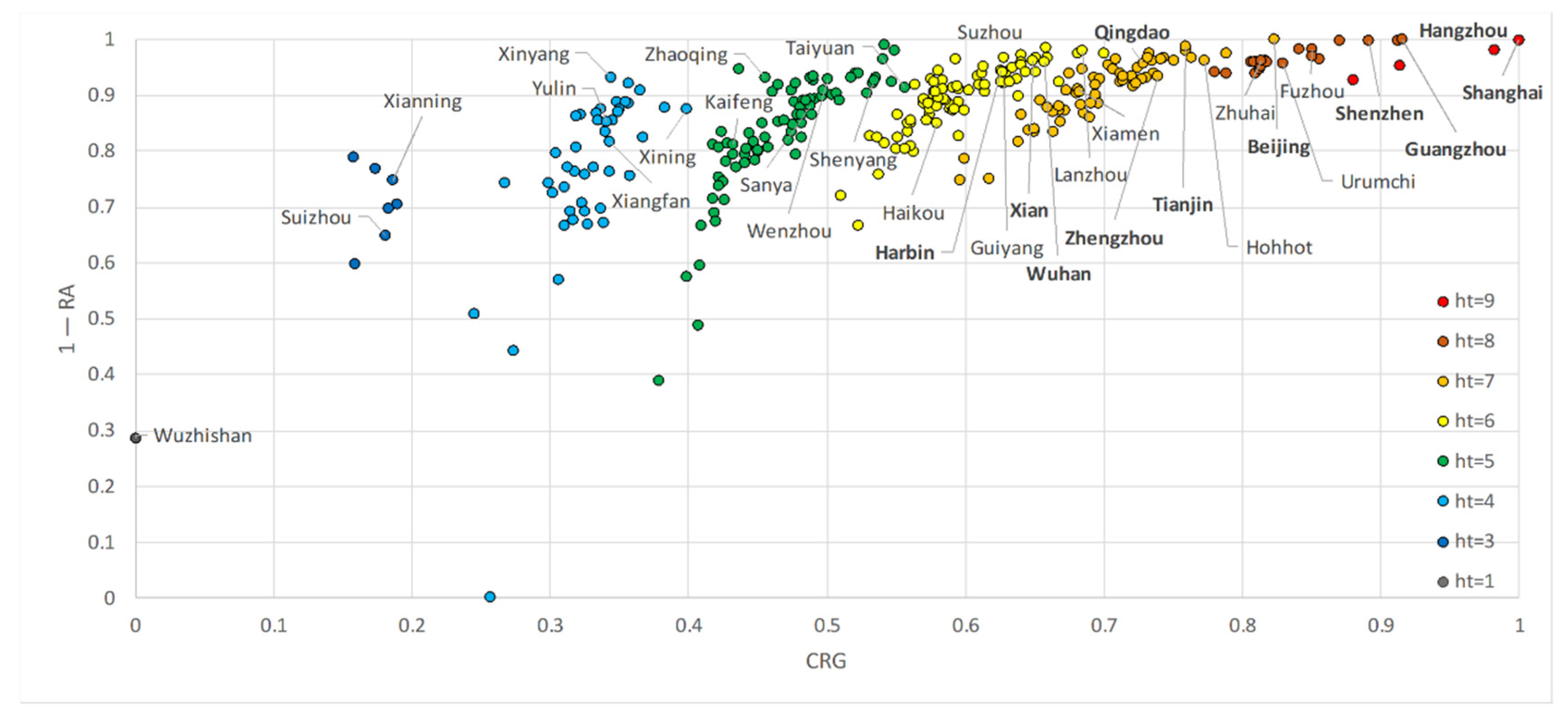
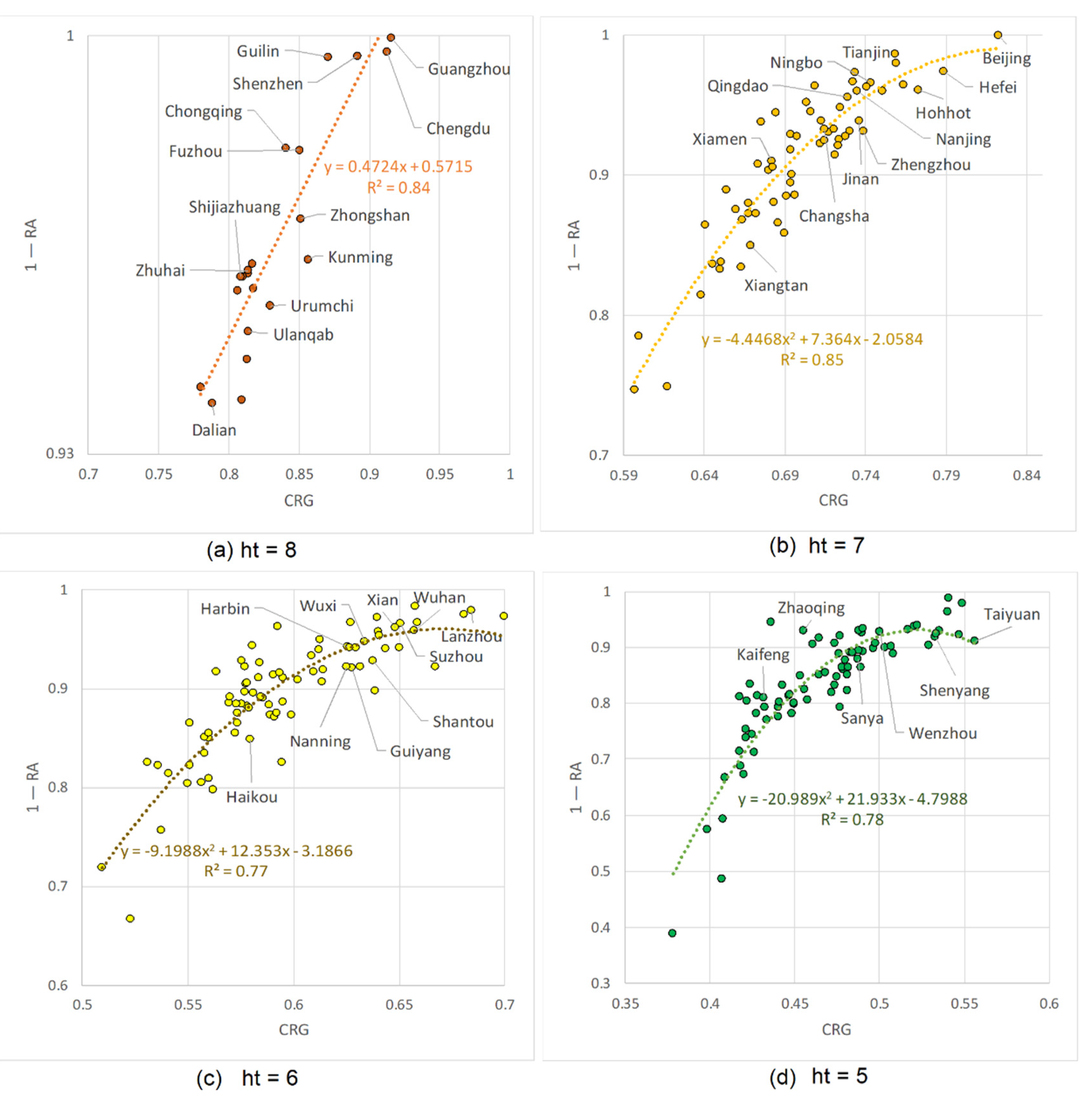
3.2. Correlations between Fractal Metrics and Urban Quantities

The investigation of how the underlying fractal pattern is related to urban quantities was conducted based on the multiple regression analysis, with the results shown in

Table 5. Multiple regression results between fractal metrics and urban quantities.

Dependant Variable	log(GDP)		log(Population)		log(CO2 emissions)
Independent Variable	Beta	Std	Beta	Std	Beta	Std
(Intercept)	3.456	0.677	2.665	0.601	1.669	0.812
log(Area)	−0.085*	0.045	0.11 **	0.040	−0.026	0.054
log(#Street)	0.639*	0.592	−0.367	0.525	1.57*	0.710
$\log \left(l_{\forall Streets}\right)$	1.66 *	4.817	1.61 **	4.278	1.02 *	5.778
ht	0.46	0.074	0.260	0.065	−0.001	0.088
CRG	0.45 *	0.052	0.140	0.046	−0.025	0.062
RA	−0.46 **	1.162	−0.31 *	1.032	0.035 **	1.394
Adjusted R Square	0.570		0.459		0.285
F-statistic	63.207		40.676		19.689
p-value	0.000		0.000		0.000

Significance level: * 0.1; ** 0.01.

. The adjust R² values are the goodness of fit for the models. Together with traditional street measures, R² values were the largest for urban GDP (0.57), followed, in order, by population (0.459) and CO₂ emissions (0.285). We also calculated the significance values using a t-test and ensured that the relationships between the independent variables and dependent variable are significant at the 1% significance level. Overall, it can be seen that the ht-index underperforms either CRG or RA with respect to the significance level. We suggest that CRG or RA being more significant than the ht-index is probably due to its increase of sensitivity.

Table 5 summarizes the effects of different types of street-configuration measures on urban socioeconomic status (log (GDP) and log (Population)) and energy consumption (log (CO₂)). The fractality of street networks is positively associated with both GDP and population, while it has a slight negative correlation with CO₂ emissions. It is interesting to note that street fractal metrics have a weaker effect than the traditional street measures, such as $l_{\forall Streets}$ and #Streets, while they have a stronger effect than city size. More specifically, a one-unit increase in $l_{\forall Streets}$ is associated with a 1.66-unit increase of urban GDP, which is about 4 times bigger than that linked with a one-unit increase in CRG. Similarly, the increase in population with a one-unit increase in $l_{\forall Streets}$ is five-fold as much as that with one-unit decrease in RA, ceteris paribus. Note that the decrease of RA is consistent with the increase of the ht-index and CRG, as smaller RA values means more striking fractals. For CO₂ emissions, a one-unit increase in street total length and number of streets is correlated with 1.02-unit and 1.57-unit increases, respectively, whereas a one-unit increase in RA (less fractal) is linked with a 0.035-unit increase.

4. Further Discussion of this Study

The augmented openness and attainability of geospatial big data helps us to analyze and grasp urban forms at both intracity and intercity levels. Street networks largely reflect an overall picture of an urban physical environment. Based on the derived natural streets over 298 cities, we can identify the fractal structure and scaling statistics of China urban street networks and further find the universal fractal pattern among a big variety of urban spaces. In this section, we further discuss the developed methodology and the obtained results and how they contribute to our knowledge in current Chinese urban studies.

Geographic features are fractal in essence, as is the urban space that involves a large collection of geographic features. The invention of the third definition of fractal [6] enables us to perceive the universal fractal pattern at various scales of geographic space. It should be stressed that given the right perspective, almost all geographic features can be seen as fractals. For example, previous work explores the underlying fractality from an individual smooth curve [1] from the very perspective of recursive bends rather than its contained vertices or segments. Similarly, for the collection of linear features—that is, the street network—one must take the perspective of street–street topology instead of segment–segment or junction–junction topology for seeing the fractal. In this study, we employed such perspective and demonstrated successfully the universal fractal pattern of street networks among over 298 cities.

The detected universal fractal pattern of urban street networks can be captured quantitatively by the power-law distribution of street connectivities and the underlying scaling hierarchies. Power-law distribution is widely observed in natural and societal phenomena, and it is usually regarded as an indicator for sustainability [29]. The power-law detection for each city was conducted using the robust maximum likelihood estimation method and helps us identify that about 67% of Chinese urban street networks hold a power law nature. For the remaining 33% of cities, the scaling hierarchical levels derived from head/tail breaks show, as well, the striking fractal patterns of far more less-connected streets than well-connected ones. Thus, the ht-index is superior to power-law metrics with respect to the identification of the universal fractal pattern of Chinese street networks. Besides, the ht-index is good for discriminating urban street networks across different scaling hierarchies; its two alternatives, CRG and RA, help us to differentiate the cities within the same scaling hierarchy because of the increment of sensitivity. In this regard, the integration of three fractal measures can provide us with a more comprehensive and also a more precise picture of fractal cities in China.

The study also attempted to estimate the explanatory power of the fractality of street networks on urban socioeconomic status and fuel consumption. As the urban indicators such as GDP are normally associated with multiple factors of a street network, the study adopted the multiple regression approach by involving other traditional street-network geometric measures in order to make the model closer to the reality and reduce the probability of confounding effects. As a result, the correlation coefficient R² value of the multiple regression model, as in the case with GDP (R² = 0.57), is higher than that of a single regression model based on one single street geometric property or fractal metric (e.g., R² = 0.41 with $l_{\forall Streets}$ only or R² = 0.23 with CRG only). Therefore, it can be said that multiple street-network measures are suitable for an exploratory analysis of each urban quantity than that of a single measure.

Our multiple regression analysis further suggests that cities with more strikingly fractal street patterns (i.e., more scaling hierarchical levels of their street networks) tend to have better economic status. The fractal analysis results in Table 4 also confirm that those most fractal cities are top-tier metropolitans in China such as Beijing and Shanghai. If we take a closer look at the coefficient $\beta$, it should be noted that the positive effect of $l_{\forall Streets}$ to urban socioeconomic status is stronger than any of three fractal metrics. This indicates that a city’s economic development is more directly represented by the geometric details of its street network than by the underlying fractal pattern. However, it does not mean that the fractal metrics are less meaningful. As shown by the regression analysis results with CO₂ emissions, the fractal structure of a street network can contribute to the energy efficiency of a city. The opposite signs of $\beta$ between fractal metrics and $l_{\forall Streets}$ indicate that street fractalities can perform differently from street geometric properties. In this regard, the fractality of street networks can be a useful supplement to traditional street-network configuration measures.

5. Conclusions

A city is not only comprised of traffic zones or buildings, but also the collection of individual coherent streets. This article explores the universal fractal pattern of 298 cities in China from the perspective of street networks. The paper applies an integration of three fractal metrics—ht-index, CRG, and RA—for fractal or scaling analysis of street connectivities. The results show that almost all cities bear a fractal structure, as the number of scaling hierarchical levels of the street network for each city is above or equal to 3. We have proven that CRG and RA can greatly compensate for the insensitivity of the ht-index. Besides, the multiple regression analysis results suggest that the fractal structure of the urban street network positively correlates with urban socioeconomic status and negatively correlates with urban energy consumption. Further research will focus on the application of the universality of fractal pattern under the framework of the third definition to the urban planning or policy-decision making by involving other geometric (such as azimuth) and structural properties (such as betweenness) of street networks and more detailed urban indicators.

References

1. Ma, D.; Jiang, B. A smooth curve as a fractal under the third definition. Cartographica 2018, 53, 203–210. [Google Scholar] [CrossRef] [Green Version]
2. Boeing, G. Measuring the complexity of urban form and design. Urban Des. Int. 2018, 23, 281–292. [Google Scholar] [CrossRef] [Green Version]
3. Gao, P.; Cushman, S.A.; Liu, G.; Ye, S.; Shen, S.; Chang, C. Fracl: A tool for characterizing the fractality of landscape gradients from a new perspective. ISPRS Int. J. Geo-Inf. 2019, 8, 466. [Google Scholar] [CrossRef] [Green Version]
4. Koch, H. Sur une courbe continue sans tangent, obtenue par une construction géométrique élémentaire on a continuous curve without tangents constructible from elementary geometry. Arkiv Matematik 1904, 1, 681–704. [Google Scholar]
5. Mandelbrot, B. How long is the coast of Britain? Statistical self-similarity and fractional dimension. Science 1967, 156, 636–638. [Google Scholar] [CrossRef] [PubMed] [Green Version]
6. Jiang, B.; Yin, J. Ht–index for quantifying the fractal or scaling structure of geographic features. Ann. Assoc. Am. Geogr. 2014, 104, 530–541. [Google Scholar] [CrossRef]
7. Batty, M.; Longley, P. Fractal Cities: A Geometry of Form and Function; Academic Press: London, UK, 1994. [Google Scholar]
8. Batty, M.; Carvalho, R.; Hudson-Smith, A.; Milton, R.; Smith, D.; Steadman, P. Scaling and allometry in the building geometries of Greater London. Eur. Phys. J. B 2008, 63, 303–314. [Google Scholar] [CrossRef]
9. Tannier, C.; Thomas, I.; Vuidel, G.; Frankhauser, P. A fractal approach to identifying urban boundaries. Geogr. Anal. 2011, 43, 211–227. [Google Scholar] [CrossRef]
10. Tannier, C.; Thomas, I. Defining and characterizing urban boundaries: A fractal analysis of theoretical cities and Belgian cities. Comput. Environ. Urban Syst. 2013, 41, 234–248. [Google Scholar] [CrossRef]
11. Thomas, I.; Frankhauser, P. Fractal dimensions of the built-up footprint: Buildings versus roads. Fractal evidence from Antwerp (Belgium). Environ. Plan. B Urban Anal. City Sci. 2013, 40, 310–329. [Google Scholar] [CrossRef]
12. Shreevastava, A.; Rao, P.S.C.; McGrath, G.S. Emergent self-similarity and scaling properties of fractal intra-urban heat islets for diverse global cities. Phys. Rev. E 2019, 100, 032142. [Google Scholar] [CrossRef] [PubMed] [Green Version]
13. Shen, G. Fractal dimension and fractal growth of urbanized areas. Int. J. Geogr. Inf. Sci. 2002, 16, 419–437. [Google Scholar] [CrossRef]
14. Mohajeri, N.; Gudmundsson, A. The evolution and complexity of urban street networks. Geogr. Anal. 2014, 46, 345–367. [Google Scholar] [CrossRef]
15. Nilsson, L.; Gil, J. The signature of organic urban growth. In The Mathematics of Urban Morphology; D’Acci, L., Ed.; Birkhäuser: Basel, Switzerland, 2019; pp. 93–121. [Google Scholar]
16. Wu, L.; Zhi, Y.; Sui, Z.; Liu, Y. Intra-urban human mobility and activity transition: Evidence from social media check-in data. PLoS ONE 2014, 9, e97010. [Google Scholar] [CrossRef] [Green Version]
17. Ma, D.; Toshihiro, O.; Oki, T.; Jiang, B. Exploring the heterogeneity of human urban movements using geo-tagged tweets. Int. J. Geogr. Inf. Sci. 2020. [Google Scholar] [CrossRef]
18. Jiang, B.; Ren, Z. Geographic space as a living structure for predicting human activities using big data. Int. J. Geogr. Inf. Sci. 2019, 33, 764–779. [Google Scholar] [CrossRef] [Green Version]
19. Porta, S.; Crucitti, P.; Latora, V. The network analysis of urban streets: A dual approach. Physica A 2006, 369, 853–866. [Google Scholar] [CrossRef] [Green Version]
20. Crucitti, P.; Latora, V.; Porta, S. Centrality measures in spatial networks of urban streets. Phys. Rev. E 2006, 73, 036125. [Google Scholar] [CrossRef] [Green Version]
21. Kirkley, A.; Barbosa, H.; Barthelemy, M.; Ghoshal, G. From the betweenness centrality in street networks to structural invariants in random planar graphs. Nat. Commun. 2018, 9, 2501. [Google Scholar] [CrossRef]
22. Jiang, B.; Claramunt, C. Topological analysis of urban street networks. Environ. Plan. B Plan. Des. 2004, 31, 151–162. [Google Scholar] [CrossRef] [Green Version]
23. Ma, D.; Omer, I.; Sandberg, M.; Jiang, B. Why topology matters in predicting human activities? Environ. Plan. B Urban Anal. City Sci. 2019, 46, 1298–1313. [Google Scholar] [CrossRef]
24. Zhang, H.; Li, Z. Fractality and self-similarity in the structure of road networks. Ann. Assoc. Am. Geogr. 2012, 102, 350–365. [Google Scholar] [CrossRef]
25. Lu, Z.; Zhang, H.; Southworth, F.; Crittenden, J. Fractal dimensions of metropolitan area road networks and the impacts on the urban built environment. Ecol. Indic. 2016, 70, 285–296. [Google Scholar] [CrossRef] [Green Version]
26. Lan, T.; Li, Z.; Zhang, H. Urban allometric scaling beneath structural fractality of road networks. Ann. Assoc. Am. Geogr. 2019, 109, 943–957. [Google Scholar] [CrossRef]
27. Crooks, A.T.; Croitoru, A.; Jenkins, A.; Mahabir, R.; Agouris, P.; Stefanidis, A. User-generated big data and urban morphology. Built Environ. 2016, 42, 396–414. [Google Scholar] [CrossRef]
28. Boeing, G. Spatial information and the legibility of urban form: Big data in urban morphology. Int. J. Inf. Manag. 2019, 102013. [Google Scholar] [CrossRef] [Green Version]
29. Salat, S.; Bourdic, L. Urban complexity. scale hierarchy, energy efficiency and economic value creation. In The Sustainable City VII: Urban Regeneration and Sustainability; Pacetti, M., Passerini, G., Brebbia, C.A., Latini, G., Eds.; WIT Press: Boston, MA, USA, 2012; Volume 155, pp. 97–107. [Google Scholar]
30. Gao, P.C.; Liu, Z.; Xie, M.H.; Tian, K.; Liu, G. CRG index: A more sensitive ht-index for enabling dynamic views of geographic features. Prof. Geogr. 2016, 68, 533–545. [Google Scholar] [CrossRef]
31. Gao, P.C.; Liu, Z.; Tian, K.; Liu, G. Characterizing traffic conditions from the perspective of spatial-temporal heterogeneity. ISPRS Int. J. Geo–Inf. 2016, 5, 34. [Google Scholar] [CrossRef] [Green Version]
32. GEOFABRIK. Available online: http://download.geofabrik.de/ (accessed on 10 November 2019).
33. National Resources and Environment Database of the Chinese Academy of Sciences. Available online: http://www.resdc.cn/ (accessed on 15 November 2019).
34. Liu, H.; Jiang, D.; Yang, X.; Luo, C. Spatialization approach to 1km grid GDP supported by remote sensing. Geo-Inf. Sci. 2005, 7, 120–123. [Google Scholar]
35. Cai, B.; Wang, J.; Yang, S.; Mao, X.; Cao, L. China City CO2 emission dataset: Based on the China high resolution emission gridded data. China Popul. Resour. Environ. 2017, 27, 7085–7093. (In Chinese) [Google Scholar]
36. Cai, B.; Liang, S.; Zhou, J.; Wang, J.; Cao, L.; Qu, S.; Xu, M.; Yang, Z. China high resolution emission database (CHRED) with point emission sources, gridded emission data, and supplementary socioeconomic data. Resour. Conserv. Recycl. 2018, 129, 232–239. [Google Scholar] [CrossRef]
37. Jiang, B.; Zhao, S.; Yin, J. Self-organized natural roads for predicting traffic flow: A sensitivity study. J. Stat. Mech. Theory Exp. 2008, 2008, 07008. [Google Scholar] [CrossRef] [Green Version]
38. Newman, M.E.J. The structure and function of complex networks. SIAM Rev. 2003, 45, 167–256. [Google Scholar] [CrossRef] [Green Version]
39. Jiang, B. Head/tail breaks: A new classification scheme for data with a heavy–tailed distribution. Prof. Geogr. 2013, 65, 482–494. [Google Scholar] [CrossRef]
40. Newman, M.E.J. Power laws, Pareto distributions and Zipf’s law. Contemp. Phys. 2005, 46, 323–351. [Google Scholar] [CrossRef] [Green Version]
41. Clauset, A.; Shalizi, C.R.; Newman, M.E.J. Power-law distributions in empirical data. SIAM Rev. 2009, 51, 661–703. [Google Scholar] [CrossRef] [Green Version]
42. Zünd, D.; Bettencourt, L.M.A. Growth and development in prefecture-level cities in China. PLoS ONE 2019, 14, e0221017. [Google Scholar] [CrossRef]
43. Mohajeri, N.; Gudmundsson, A.; French, J.R. CO2 emissions in relation to street-network configuration and city size. Transp. Res. Part D Transp. Environ. 2015, 35, 116–129. [Google Scholar] [CrossRef]
Figure 1. (Color online) Spatial distribution of (a) selected 298 cities, (b) national street network, and (c) the methodological framework in this study.
Ijgi 09 00192 g001
Figure 2. (Color online) Transformation from segment–segment topology to street–street topology. (Note: From the network perspective of street segments and streets, segment–segment topology (Panels a and b) is a mechanistic structure that lacks the scaling pattern of far more smalls than larges, whereas the street–street topology (Panels c and d) is organic, as it holds such a pattern clearly).
Ijgi 09 00192 g002
Figure 3. (Color online) The geometric shapes of first three iterations of Koch curve (a) and their underlying scaling statistics to illustrate three fractal metrics. Note: (b) is the power law relationship between the number of segments and scales; (c) ranks all the scales from the largest to the smallest for calculations of ht-index and CRG; (d) Two types of areas in the rank-size plot for the calculation of RA
Ijgi 09 00192 g003
Figure 4. (Color online) Using the first five iterations of the Koch curve to illustrate CRG and RA supplementing the ht-index in terms of capturing sensitivity.
Ijgi 09 00192 g004
Figure 5. Power-law distributions of #segments and #streets per city (note: # = number).
Ijgi 09 00192 g005
Figure 6. (Color online) An integrated view of CRG and RA of street connectivities for 298 cities. (Note: names of top cities by GDP are in bold).
Ijgi 09 00192 g006
Figure 7. (Color online) The correlation between CRG and RA for cities with the same ht-index. Note: Panels (a), (b), (c), and (d) are correlations with the ht-index of 8, 7, 6, and 5, respectively.
Ijgi 09 00192 g007
Figure 8. (Color online) The fractal pattern of far more less-connected streets than well-connected ones across top 20 cities by GDP in China. (Note: A spectrum of color is adopted to visualize the city’s street structure, with red and blue representing the best-connected and poorest-connected streets, respectively; the other colors (in cyan, yellow, and orange) represent the streets in between).
Ijgi 09 00192 g008