Abstract
The requirements of location-based services have generated an increasing need for up-to-date digital road maps. However, traditional methods are expensive and time-consuming, requiring many skilled operators. The feasibility of using massive GPS trajectory data provides a cheap and quick means for generating and updating road maps. The detection of road intersections, being the critical component of a road map, is a key problem in map generation. Unfortunately, low sampling rates and high disparities are ubiquitous among floating car data (FCD), making road intersection detection from such GPS trajectories very challenging. In this paper, we extend a point clustering-based road intersection detection framework to include a post-classification course, which utilizes the geometric features of road intersections. First, we propose a novel turn-point position compensation algorithm, in order to improve the concentration of selected turn-points under low sampling rates. The initial detection results given by the clustering algorithm are recall-focused. Then, we rule out false detections in an extended classification course based on an image thinning algorithm. The detection results of the proposed method are quantitatively evaluated by matching with intersections from OpenStreetMap using a variety of distance thresholds. Compared with other methods, our approach can achieve a much higher recall rate and better overall performance, thereby better supporting map generation and other similar applications.
1. Introduction
With the development of the Internet and smart phones, LBSs (location-based services) have become a fundamental part of people’s daily lives, increasing a general need for detailed and up-to-date digital road maps. However, conventional map-producing methods are very time-consuming and labor-intensive, as both field surveys and map construction involve many skilled operators. Meanwhile, due to rapid changes in real-world road networks, newly generated road maps may quickly become out-of-date. The company TomTom once estimated that, every year, up to 15% of roads need to be updated [1]; for developing countries, this percentage may be even higher. Therefore, companies such as Google, Apple, TomTom, Baidu, and so on, have large teams which manually collect road data using costly techniques, from car mapping to remote sensing. Automatic road extraction from aerial and satellite imagery has been studied extensively over the past 30 years [2,3], along with road extraction from light detection and ranging (LiDAR) point-cloud data [4]. However, these approaches are susceptible to surrounding objects (e.g., cars) occluding the road, which results in discontinuities in the extracted road [2]. Moreover, the acquisition of remote sensing images and point-cloud data is very expensive and has a lag in transmission and processing. With the development of Internet and GPS technologies, an individual can record their trajectories using GPS devices, which are now common in vehicles and smart phones, and contribute them to a dataset called volunteered geographic information (VGI) data with fast uploading and updating speeds [5]. Given their crowd-sourced attributes, publicly available GPS trajectory datasets serve as good supplementary resources for map production. The recent surge in accessible GPS trajectory data and automatic map generation algorithms has made inexpensive map construction and real-time map updating possible [6]. Automatically generating high-quality and real-time road maps from GPS trajectory data is an active research topic, which urgently needs to be addressed.
At present, an increasing number of vehicles are equipped with GPS devices, making it feasible to acquire a large collection of real trajectories remaining on roads. One publicly available dataset contains 14,716 taxis and over 75 million GPS points in the Chinese city Shenzhen, recorded over only one day [7]. From massive vehicle trajectory data, the underlying geometries, and topologies of the road network can be inferred by capturing the similarities between trajectories. For example, a location at which many vehicles have turned (presented as a turn-point in the corresponding GPS trajectory) is very likely to be an intersection of a road network. Semantic information (such as number of road lanes, volume of traffic flow, and turning restrictions) of roads can also be extracted by mining collective mobility patterns from these data [8,9,10], contributing to the construction of a highly detailed road map. More importantly, the whole process (i.e., from positioning and collecting data to generating a road map) is automatic.
However, automatically generating road maps from GPS trajectory data can be very challenging, due to the low sampling rates and disparities of coverage involved. First, to save energy and communication costs, low-frequency (average sampling interval over 20 s) trajectories are ubiquitous among floating car data, such as data from taxis, shuttles, and so on. These low sampling rates cause GPS trajectories to not accurately depict the motion of vehicles (e.g., the nearest GPS point to an actual turning spot may be over 10 s and 100 m away). Second, disparities make it hard for existing algorithms to distinguish a real road traveled by very few trajectories from a false one. Spurious roads are common in generated maps, due to the fluctuating GPS noise caused by complex urban environments, and it is currently infeasible to determine a good enough global threshold for removing them. As a result, when using low-frequency trajectory data collected by floating cars, the generated map is often poor in quality and coverage. Maps generated from high-quality trajectory data collected by experimental cars can only cover very limited routes and, thus, are impractical.
To address these challenges, methods taking global trajectory information into consideration have been proposed [10,11,12], which are aimed at achieving better detection and extraction of the elements forming a road map. A few methods have also managed to utilize the geometric features of road at the same time [11,12]. In a road map, road intersections (regions where three or more road branches converge) are critical elements which hold valuable semantic information, such as turning restrictions. As one can readily construct a road map with its topological structure by connecting known road intersections, road intersection detection from GPS trajectory data is a prerequisite for a category of map generation methods [6] and remains a key problem in map generation.
Given their geometric and topological features, road intersections can be recognized by algorithms effectively and automatically. Still, their detection faces the same low sampling rate and disparity challenges mentioned above. To the best of our knowledge, no existing studies have achieved both high precision and high recall rate in detecting road intersections from low-frequency GPS trajectory data; furthermore, most of them were precision-focused [10,13,14]. In many applications, missing an intersection is less tolerable than returning a deviated position, which calls for research focused on higher detection recall rates.
Therefore, we propose a novel three-step approach to detect road intersections from low-frequency trajectory data, focusing on improving recall rate with an acceptable precision. The major contributions of our method include:
- (1)
- We introduce a stay-point detection algorithm in the pre-processing course to remove a large proportion of false turn-points not indicating road intersections, which few methods have considered before;
- (2)
- We propose a turn-point compensation algorithm, which utilizes geometric and hot area features of road intersection. This algorithm retrieves actual turning positions from low-frequency trajectories using a turning angle assumption determined by the density map of all GPS points. An indicator to evaluate the quality of a selected turn-point is presented, proving that the concentration of turn-points is significantly improved by our pre-processing and position compensation processes;
- (3)
- We extend the point clustering-based road intersection detection framework to include a post-classification course. The clustering algorithm first yields a recall-focused detection result, following which the classifier greatly increases the detection precision by utilizing the geometric features of road intersections, with a small cost in recall rate due to misclassification. The extended classification course makes the overall performance of our method better than that of existing precision-focused methods, and it is easy to implement co-operatively with any recall-focused detection algorithm.
Our paper is organized as follows: Section 2 reviews the related work on detecting road intersections from GPS trajectory data. Section 3 describes the proposed three-step road intersection detection method. Section 4 presents a set of experimental results and analyses. Finally, our conclusions are discussed in the last section.
2. Related Work
The abundance of GPS trajectory data and an increasing need to generate up-to-date digital road maps have led to a recent surge in research of map generation algorithms using trajectory data [6]. Most of these methods first extract road segments or road intersections from a batch of trajectories and, then, construct a road network by connecting them [8,11,12,13,14,15]. A few methods insert every trajectory into an existing map to build the whole structure incrementally, relying heavily on high-quality input data [16]. When it comes to low-frequency trajectory data, methods making use of the spatial aggregation of massive trajectory data perform better, in general. A road map is typically represented by a directed graph, where road intersections can be abstracted as nodes incident to no less than three connected edges.
Given their geometric and topological features, road intersection detection is a key problem in map generation. The first GPS trajectory data-based map generation method was proposed by Edelkamp and Schrödl [8]. In their subsequent work, a refined road intersection model was introduced to support the extraction of turning restrictions [15]. Karagiorgou defined a turn-point as a GPS point where a vehicle reduces its speed and changes its direction significantly; based on this idea, a turn-point clustering-based road intersection detection method was presented [13], in which map construction was carried out by connecting detected road intersections. Therefore, detection precision and recall are crucial in ensuring that the constructed map is of high quality. Experiments showed that assembled turn-points could indicate road intersections well. Recently, Deng’s work included generating detailed structure models of road intersections [10], which captured the complexity of realistic road networks and could support smarter navigation algorithms. This makes road intersection detection even more crucial.
Existing road intersection detection methods can be roughly divided into three categories: (1) point clustering methods, which seek particular trajectory points indicating road intersections and, then, apply clustering algorithms to detect existing intersections. Karagiorgou’s method used the clustering of turn-points [13]; following which, Wu using a stricter turning angle threshold in turn-point selection [14]. Deng’s method introduced a local G* statistic, taking nearby point’s heading direction into consideration to select candidate points indicating road intersections [10]. Zhang’s method detected road intersection by finding the “node” pixels in the skeleton of a road image which is generated by rasterization based on all GPS points, utilizing the topological feature of the junction of roads [12]. (2) Classification-based methods turn the detection problem into an object recognition problem (mostly based on a shape descriptor), applying a classification algorithm to determine whether a candidate region is a road intersection or not. Fathi’s method used circular bins as a shape descriptor; the classifier was trained by the Adaboost algorithm [17]. Chen’s method developed a traj-SIFT descriptor, then trained a multi-class Support Vector Machine (SVM) classifier over this descriptor [11]. (3) Trajectory pattern mining methods locate intersections by finding the divergence of two groups of similar trajectories. In Xie’s method, the similarity between trajectories was calculated based on the longest common subsequence (LCSS) [18].
However, there are two main challenges in road intersection detection: (1) the low sampling rate and (2) the high disparity of trajectory data. First, low sampling rates greatly increase the uncertainty of trajectory data; existing methods which mine vehicle motion patterns to detect road intersections typically suffer from huge information loss. Second, high disparities cause algorithms to tend to mistake intersections passed by very few trajectories as outliers. Finding a global threshold to separate false detections from correct ones is currently infeasible. To address these challenges, our method adapts both the geometric features of road intersections and features of being hot areas of GPS points, which are both robust against low sampling rates.
Our method follows Karagiorgou’s approach; that is, using turn-points to detect road intersections. However, differing from previous works, we carefully examine the ability of these points to indicate road intersections under low sampling rates. We quantify this ability by calculating the proportion of turn-points falling within an intersection region. Experiments show that not only can a low sampling rate cause turn-points deviating from the actual turning position, but a large amount of stay-points can be mistaken for turn-points; both of which severely damage turn-points’ ability to indicate road intersections. Therefore, both position compensation and pre-processing are needed to solve this problem. Moreover, our detection method is recall-focused, a loose threshold is used in the clustering algorithm, and we found that the post-classification course collaborates well with the recall-first approach. The classifier receives limited candidate intersection regions from the initial clustering results, and its classification accuracy guarantees a lower bound on the final detection precision. The loss of recall rate due to misclassifying a true intersection is rather small, compared to applying a strict global threshold in the clustering algorithm. As it is based on a classic image-thinning algorithm, our classifier is easy to implement and can co-operate with any recall-focused detection method.
3. Road Intersection Detection from Low-Frequency Trajectory Data
Considering the movement of a vehicle, its turning points can indicate existing road intersections well. However, for low-frequency trajectory data, this ability is severely degraded. Therefore, we propose a novel three-step approach to detect road intersections using refined turn-points generated by a position compensation algorithm. The three steps are trajectory segmentation, clustering turn-points after compensation, and road intersection classification.
A GPS trajectory is a sequence of GPS points . Table 1 shows the five essential attributes comprising each GPS point. Within these attributes, speed is the magnitude of vehicle’s velocity and heading is the (clockwise) angle of its direction. When a vehicle is moving in the direction of Earth’s true north, its heading is equal to 0. However, not every GPS system records speed and heading; thus, in our method, these two attributes are always estimated using the current point and its predecessor (if it exists).

Table 1.
Attributes of each GPS point .
Among these five attributes, speed and heading are derived from the other three attributes, and mainly being used in selecting turn-points. One may think that better estimations can be calculated using more GPS points, however it is very challenging to do so under the low sampling rate. In conclusion, the high uncertainty of low-frequency trajectory data consists of both space-time uncertainty and motion uncertainty, resulting in deviation between a turn-point and vehicle’s actual turning position along with biased speed and heading attributes. Our method first tries to prevent more false turn-points from being selected under the low sampling rate. The deviation problem is later mended using the position compensation algorithm.
3.1. Trajectory Segmentation Based on Stay-Point Detection
When dealing with low-frequency trajectory data, pre-processing is very necessary to prevent false turn-points from being selected. A false turn-point has a significant change in speed and heading due to GPS noise, but does not correspond to a real turn and can never be calibrated. Clustered false turn-points typically result in false road intersection detections and position shifting of correct intersections. In pre-processing, previous methods have included using an abnormal-distance threshold to split a trajectory into two parts [19], or an N-successive abnormal-turning rule to mark such trajectories as outliers [10]. However, when vehicles are stranded in traffic jams, a large amount of false turn-points are generated, which has not been considered yet, to our knowledge.
When a vehicle stays in a fixed location, the positioning results are randomly spread within a small region, leading to fluctuations in heading directions estimated from successive GPS points. Neither an angle threshold nor a speed threshold can prevent these stay-points from being selected as turn-points, even though the vehicle does not turn. Therefore, we introduce a stay-point detection algorithm to first group successive stay-points into segments; thus, each trajectory is segmented into normal points and groups of stay-points. Figure 1 shows an example of successive stay-points being detected in a trajectory.
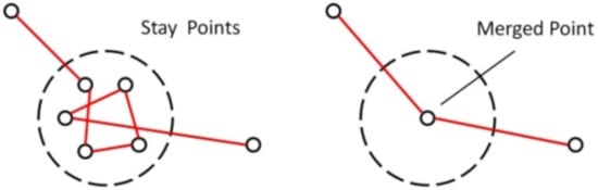
Figure 1.
Merging detected stay-points in a trajectory.
In general, starting with an anchor point , the stay-point detection algorithm first returns the longest sequence of successors satisfying . Then, if the time span between and the last successor is larger than a given threshold, a stay-point (containing a series of GPS points) is detected [20]. The algorithm then starts detecting the next stay-point from . However, as the input trajectory here is of low frequency, a unified speed threshold performs better than the distance and time span thresholds detailed above. Therefore, in this paper, a stay-point speed threshold of 1 m/s and an abnormal speed threshold of 55.5 m/s (equal to 200 km/h) were used. Figure 2 shows the distribution of detected stay-points from the Shenzhen taxi trajectories: one can see that they are quite different from the ideal turn-point regions, which are supposed to indicate road intersections. If a turn-point selected by Karagiorgou’s criterion [13] is also a stay-point as found using our pre-processing method, we count it as a false turn-point. In a quick test, it turned out that more than 50% of turn-points were false and, when we used Wu’s (stricter) criterion [14], that percentage was even higher.
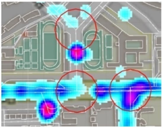
Figure 2.
Kernel density estimation of stay-points. The red circles are regions with road intersection.
We demonstrated that stay-points cannot reliably indicate road intersections and that false turn-points are easily mistaken for turn-points by existing methods. However, we still want to keep the information of detected stay-points, as they do make true statements about vehicle positions. Therefore, successive stay-points are merged into one point (Figure 1), represented by their center position . The merged point keeps two timestamps , as we need to estimate the speed at the merged point and for the next point. Once we recalculate the merged point’s attributes (Table 1), it can be selected as a turn-point like a normal GPS point. The filtered turn-points can reflect road intersections more correctly and the burden on the clustering algorithm is significantly reduced, especially when dealing with massive trajectory data.
3.2. Clustering Turn-Points after Position Compensation
Following pre-processing, we select turn-points from input trajectories using an angle threshold and a speed threshold for turn-points, which have shown good performance in indicating road intersections. As we are dealing with massive low-frequency data, stricter thresholds (compared with Karagiorgou’s criterion) are preferred, since they yield a lighter and more reliable turn-point set. Here, an angle threshold of 45° and a speed threshold of 10 m/s are used, as determined by a series of experiments on the Shenzhen taxi dataset. Before clustering, we need to take a closer look at the ability of turn-points to indicate road intersections (Figure 3).
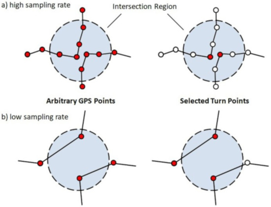
Figure 3.
Turn-point’s ability to indicate a road intersection.
We present an indicator to quantify specific points’ ability to indicate a road intersection. Given a ground truth road intersection and its center position (as offered by OpenStreetMap [21]), the intersection region is defined as a circle with radius of . Then, regions of existing road intersections are joined together (Equation (1)) for convenience, in order to determine whether a point falls within a road intersection region.
For a point set , the indicator is calculated by the following equation:
Clearly, the higher is, the more points in the point set are scattered near an existing intersection, which suggests that clusters of these points can represent road intersections. With this indicator, we can better answer the following two questions: How well does a batch of turn-points indicate road intersections? Is that ability degraded under a low sampling rate? Table 2 shows comparative results using high-frequency trajectory data from Chicago [6] and low-frequency data from Shenzhen [7]. The radius of road intersection was empirically set as 50 m.
Table 2.
Comparative result of using high-frequency and low-frequency trajectory data.
For the Chicago campus bus dataset (average sampling interval 3.6 s), over 90% of the selected turn-points fell within an intersection region while, for arbitrary trajectory points, that percentage was merely 33.84%. Thus, turn-points do have good ability in indicating road intersections. However, for the Shenzhen taxi dataset (average sampling interval 26.1 s), the corresponding percentage of turn-points dropped from 90.30% to 50.14%, showing no particular advantages over arbitrary points. If one insists on using turn-points to detect road intersections under such circumstance, this indicator must be improved by some means. As we know, the underlying reason is that GPS points cannot accurately depict vehicular motion, thus, using stricter angle and speed thresholds in turn-point selection cannot solve this problem. Therefore, we propose a position compensation algorithm to place the turn-points in the vehicle’s actual turning positions.
3.2.1. Turn-Point Compensation Based on Turning Angle Assumption
As mentioned earlier, when a vehicle turns, the closest GPS point can be over 10 s earlier or later than that moment under a low sampling rate. Thereby, a recorded turn-point may deviate from the nearest intersection’s center position by over 100 m, given the average moving speed of vehicles. The goal of turn-point compensation is correcting for such deviations caused by low frequency rates, as a clustering algorithm can produce better detection results with a better input. As one cannot tell when a vehicle is turning from the trajectory data, finding the turn position relies on utilizing geometric information.
In Wu’s method [14], a pair of consecutive turn-points is required to determine the vehicle’s entering vector and leaving vector when traversing an intersection. The actual turning position is calculated as the convergence of the two prolonged vectors (Figure 4a). Apparently, not all turn-points can meet this strict requirement. Instead of using two vectors, our method only uses the entering or leaving vector, combined with a set of turning angle assumptions (Figure 4b).
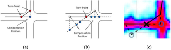
Figure 4.
Turn-point compensation process: (a) compensation position by Wu’s method; (b) series of candidate positions by our method; (c) density map helps to determine the optimal turn-point.
The turning angle assumption comes from the common-sense assumption that a vehicle turning must follow the restriction of the intersection’s shape. As a 90 assumption can only cover T- and cross-shaped road intersections, a set of turning angle assumptions are used. The set is obtained by interpolating between the minimum and maximum legitimate turn angles; here, we use [30,150], along with an angle interval of 10. With every turning angle assumption , two compensation positions can be calculated (Equation (3)), depending on whether the timestamp of the turn-point is earlier or later than the actual turning moment:
Thus, the compensation algorithm first yields a series of candidate points . To find the optimal compensation position, our approach utilizes the hot area feature of road intersections, which few methods have considered before. Given a batch of GPS points, a density map can be calculated using the kernel density estimation (KDE) algorithm [22], assigning every location with a density value . The higher the density value is, the more likely a location is to be within a road intersection region, as a road intersection gathers the traffic volume of its connected road branches (Figure 4c). Therefore, our algorithm picks the candidate position with the highest density value as the compensated turn-point:
We experimentally found that, after the position compensation process, the indicator of the selected turn-points from the Shenzhen taxi data significantly raised, from 50.14% to 71.64%. We find that the refined turn-points are much closer to road intersection centers, in general. Therefore, the clustering algorithm can yield a better detection result.
3.2.2. Clustering Algorithm Based on Delaunay Triangulation
For the clustering algorithm, we chose the spatial clustering algorithm based on Delaunay triangulation, as the Delaunay triangulation has many useful properties related to road intersection detection. First, it keeps every point in a planar point set connected with its nearest neighbor point, capturing proximity relationships among these points with a simple graph . Furthermore, the number of edges in is at most and can be computed in time [23]. Based on a triangulation , the goal of the clustering algorithm is to find sub-graphs showing strong spatial aggregation. Figure 5 demonstrates that clusters can be found by deleting the “long” edges in based on a criterion function which takes both global and local edge lengths into consideration.

Figure 5.
Procedure of Delaunay triangulation-based clustering.
To discover clusters of arbitrary shape, existing Delaunay triangulation-based clustering algorithms typically adopt a two-step approach: first, delete the “long” edges in to roughly separate the clusters; then eliminate “bridge” edges between clusters to yield the clustering result [23]. However, finding the “bridge” edges remains a challenge. We constructed our clustering algorithm as a simplification of previous ones, given that road intersections are typically distant from each other by design. Our approach repeatedly deletes the “long” edges within each sub-graph, until every sub-graph’s radius is smaller than a given threshold. Here, the radius of a graph is defined as the radius of the smallest circle covering all planar points of the graph. The clustering algorithm consists of the following five steps:
Step 1: Calculate the Delaunay triangulation of all turn-points.
Step 2: Calculate the criterion function of each point according to Equation (5), then delete any edges connected to if its length is larger than .:
where represents the mean edge length in , represents the mean length of edges connected to , and represents the standard deviation of edge lengths in .
Step 3: Construct sub-graphs of after the “long” edges are deleted. Then, calculate every sub-graph’s radius as the radius of the smallest circle covering all points in .
Step 4: If a sub-graph’s radius is larger than a given threshold , repeat Steps 2 and 3 on that sub-graph.
Step 5: Obtain clusters of turn-points from the generated sub-graphs with more than points.
Clearly, a small enough radius threshold can separate one intersection cluster from another; here, we use m. The key parameter of this clustering algorithm is the cluster-points threshold , which represents the algorithm’s sensitivity to small samples. Figure 6 shows the variation of detection precision and recall using different cluster-points thresholds. Clusters with more turn-points are more likely to be a real intersection; however, the optimal threshold is hard to determine, due to the high disparity of the trajectory data.

Figure 6.
Detection precision and recall using different cluster-points thresholds.
Furthermore, tuning the cluster-points threshold does not add much information about the road intersection. To achieve a high recall rate covering most existing intersections, we chose a loose threshold of , comparing with the massive input trajectory data. Unsurprisingly, loosening this threshold incurred an unacceptably low detection precision. Our solution to this was extending a post-classification course which utilizes geometric information of road intersections.
3.3. Road Intersection Classification Based on Thinning Algorithm
After the clustering algorithm yields a recall-focused initial result, the last step is ruling out false detections by a road intersection classifier, raising the overall performance of the final result. Given a possible road intersection and its position, the classifier decides whether it is positive or negative using local information, instead of a global threshold. As detection precision and recall are our highest concerns, a binary classifier was chosen for our needs. We used to roughly summarize the binary classifier’s performance. Given the classification accuracy, the relationship between , the detection precision and recall before classification, and those after classification, can be seen in Equation (6). Table 3 shows simulation results relating how classification significantly changed the detection precision and recall rate.
Table 3.
Simulation result of detection precision and recall after classification.
Table 3 also demonstrates that the extended classification course combines best with recall-focused detection algorithms. Equation (6) guarantees that the detection precision after classification is no smaller than either the classification accuracy or initial detection precision: . Thereby, detection precision under the loose clustering threshold is boosted greatly, at a relatively small cost in recall rate, .
In conclusion, a well-performing classifier can promise recall-focused road intersection detection methods significant improvement in overall performance, as it utilizes more information than a global threshold. Here, we propose a binary road intersection classifier based on a classic image thinning algorithm, which requires no training and, thus, is easy to implement.
3.3.1. Road Centerline Extraction from Density Map
First, we recall the definition of a road intersection, which is a region where three or more road branches converge. Therefore, we turn binary classification into a road centerline extraction problem, as the road centerline uniquely identifies a road. Road centerline extraction from density maps has been deeply studied, using KDE-based map generation approaches [6].
In most existing approaches, a density map of GPS points is first transformed into a discrete binary image using grid-partitioning and density thresholding, such that image-processing algorithms can be applied to extract the centerline (or skeleton) from the road area image. The density threshold is used to remove noise pixels and to produce a binary road image which is both inclusive and accurate. However, due to the high disparity and GPS noise of trajectory data, it is infeasible to find an optimal global threshold [22].
The initial road intersection detection results yield a divide-and-conquer strategy to address the difficulty of selecting a density threshold. In our application, what we require are images of road intersections, not the entire road network of a city. Figure 7 demonstrates that a local density threshold is rather feasible. Given a 100 100 m area, a 1-D histogram of grid density can be produced from the density map. The median grid density serves as a good local threshold, which can filter noise pixels while keeping the road branches (see the two leftmost images in Figure 7).
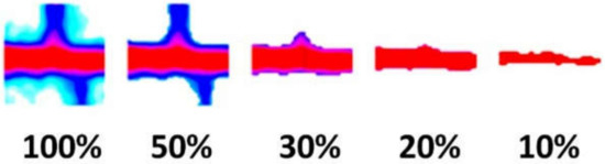
Figure 7.
Intersection images preserving different pixel ratios.
After slicing the binary image of a candidate road intersection from the density map, the next step is applying the Zhang-Suen thinning algorithm [24] to extract road centerlines within the local area. The thinning algorithm repeatedly “thins” an image until convergence. In each iteration, contour pixels of the road image are detected and removed. Whether a pixel is a contour pixel is determined by checking its eight neighboring pixels. As road edges are evenly removed by this means, road centerlines are preserved [24]. Figure 8 shows a series of road centerline extraction results from the Shenzhen taxi trajectory data.
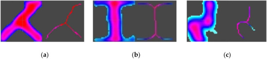
Figure 8.
Extract road centerlines by thinning an image slice; (a) from a skewed T-shaped intersection. (b) from a road segment; and (c) result with a spurious road due to GPS noise.
However there remains the spurious problem, which is common in KDE-based approaches [6,22]. Figure 8c shows that the thinning algorithm is sensitive to “bumps” along the road edge, often mistaking them for short road segments. Our solution to this problem combines a blurring-sharpening process before the thinning algorithm and a final pruning process. In the blurring-sharpening process, we first let every pixel distribute its density value to nearby pixels using a Gaussian kernel (Equation (7)); then, we apply a median density threshold once again to emphasize the road branches. This process aims to smooth the “bumps” along the road edge. Finally, the pruning process aims to remove spurious roads from the extraction result. A length threshold is introduced, and a road centerline is preserved only if it contains more than pixels.
where , is often set to 8.5 m [22], and is the grid size of a pixel, which mostly affects the running time.
3.3.2. Classifying Road Intersections Based on Road Centerlines
Given the road centerline extraction algorithm, our binary road intersection classifier consists of four steps, as follows:
Step 1: For every candidate road intersection (generated by the clustering algorithm), produce a 100 100 m density map slice around its center position.
Step 2: Transform the road intersection slice into a binary image using grid partitioning and the median density threshold.
Step 3: Extract road centerlines from the binary image using the algorithm presented in the last section.
Step 4: Find the junction points where three or more road centerlines converge. If a junction point is within ε of the center position, then classify this candidate road intersection as positive. Otherwise, classify the candidate road intersection as negative.
Here, the threshold ε represents to what degree we reject an over-deviating road intersection. We expect road centerlines to converge at the center position, but discrete junction points are not always that precise. The grid size also affects ε and . Here, the grid size was set to 2.5 m, yielding a 40 40 pixel binary image input for the road centerline extraction algorithm. We also used a rejection threshold of m and a length threshold of .
4. Experimental Results
In this section, we evaluate the quality of road intersection detection by our method using both the Chicago and Shenzhen datasets. We also verify the effectiveness of extended courses in this novel framework. Finally, a parameter analysis is also carried out.
4.1. Datasets and Detection Evaluation
Chicago Dataset. In our experiment, the Chicago dataset, which has a sample rate of 3.6 s, was used to represent high-quality data. It is a rather small dataset, covering an area of 3.0 1.9 km and containing 889 traces along with 118,360 GPS points.
Shenzhen Dataset. The Shenzhen dataset, which has a sample rate of 26.1 s, represents low-quality data. It contains over 75 million GPS points from 14,716 taxis, recorded over the course of one day [25]. In our experiments, only a subset which covers an area of 2.0 2.0 km was used. The longitude and latitude of this area’s center point is (114.08°,22.55°). The subset contains 19,906 traces and 319,601 GPS points.
Detection Precision and Recall. The road intersection detection result was evaluated by computing the precision, recall, and . A set of distance thresholds were used in matching detected intersections with the ground truths offered by OpenStreetMap [21]. Given a distance threshold , if a detected intersection’s center position was within of a ground truth’s center position, we counted it as a matched intersection. The precision, recall, and are defined as follows:
Therefore, detection precision and recall vary, according to the distance threshold; a smaller distance threshold represents higher quality demand for the generated road map. As Ahmed’s comparative work [6] used a set of distance thresholds {10, 40, 70, 100 m} in evaluating the generated map’s quality, our work followed that, using a stricter set {5, 10, 20, 40 m} in evaluating the effectiveness of the detected road intersections.
4.2. Evaluating Detection of Road Intersections
4.2.1. Chicago Dataset
For the Chicago dataset, we manually selected 50 road intersections as ground truth, each of which was traversed by at least three trajectories in the dataset (Figure 9). As the input was high-quality data, we mainly verified the effectiveness of the clustering algorithm, as well as comparing our criterion in turn-point selection with that of Karagiorgou [13].
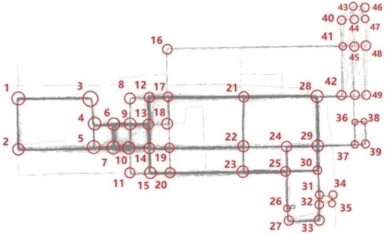
Figure 9.
Chicago dataset and existing road intersections.
As shown in Table 4, our criterion yielded fewer but more reliable turn-points, achieving a higher detection precision, especially when under the strict matching threshold. Therefore, there was no need to extend the post-classification course. However, the detection recall rate dropped, as those intersections being passed by very few trajectories were hard to detect using a strict turn-point selection criterion.
Table 4.
Detection precision and recall using the Chicago dataset.
4.2.2. Shenzhen Dataset
For the Shenzhen dataset, we focused on a 2.0 2.0 km area and manually selected 66 ground truth road intersections, each being passed by at least three trajectories (Figure 10). Using the low-frequency data, we quantitatively compared our method with the aforementioned method proposed by Karagiorgou, then verified the effectiveness of the turn-point compensation course along with the road intersection classification course. The evaluation involved no human inspection.
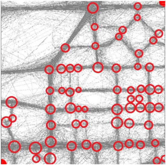
Figure 10.
Shenzhen dataset (partial) and existing road intersections.
As shown in Table 5, our method achieved significantly higher recall and , which demonstrates the superior performance of this framework in detecting road intersections. Our method can handle low-frequency trajectory data, while the method of Karagiorgou generated a large amount of false detections, even though we tuned an optimal cluster-points threshold through a series of experiments. Moreover, the method of Karagiorgou considers only the typical T-shaped and cross-shaped intersections, while our method covers arbitrarily shaped intersections.
Table 5.
Comparison of road intersection detection.
Next, we verified the effectiveness of the road intersection classification course. Figure 11a shows that the extended classification course greatly boosted detection precision at a relatively small cost, in terms of recall rate. The improved was 0.82 under a matching threshold of 40 m, which was far better than 0.67 (the one before classification). Over 90% of false detections were ruled out by our simple binary classifier, and there is ample room for further improvements.
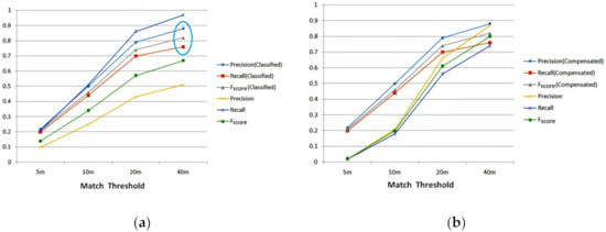
Figure 11.
Detection precision, recall, and . (a) comparing detection result with non-classified; (b) comparing detection result with non-compensated.
Finally, we verified the effectiveness of the turn-point compensation course. As shown in Figure 11b, turn-point compensation improved both detection precision and recall, as the positions of the generated road intersections were made more accurate by using a better turn-point set. Further discussion using quantitative indicators will be presented in next section. Figure 11b also shows that the turn-point compensation course had a greater effect under a strict matching threshold, which plays a critical role in generating high-quality maps.
4.2.3. Effectiveness of Key Algorithms
So far, we have verified the effectiveness of the turn-point compensation and road intersection classification courses using the detection precision, recall, and . Next, we introduced two quantitative indicators to verify the effectiveness of the key algorithms in our three-step approach.
First, we recall the experiment shown in Figure 3, where the indicator was defined as the ratio of turn-points within meters of an intersection’s center. A higher value means that turn-points are more concentrated on a road intersection, helping the clustering algorithm to yield better detection results. Figure 12 shows that, when using both position compensation and trajectory segmentation algorithms (orange curve), a significant improvement in concentration of turn-points was achieved. The indicator of selected turn-points increased from 50.14% to 71.64%, which verifies the effectiveness of these two algorithms.
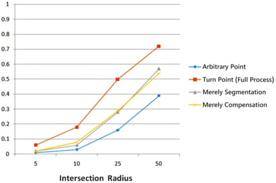
Figure 12.
Variation of indicator .
Moreover, when merely using the position compensation algorithm (yellow curve), the improvement of a larger group of turn-points was trivial, as no information can be drawn from compensating for a large proportion of turn-points which were false. The same phenomenon happened when merely using the segmentation algorithm (grey curve), the improvement was also trivial, as removing false turn-points cannot make the remaining ones more accurately depict vehicular motion. Therefore, these two algorithms must be jointly used to achieve full usage.
The next indicator was the classification accuracy, of the binary road intersection classifier. Table 6 shows details of our image thinning algorithm-based classifier’s performance, from which we can see that the classifier tended to make more mistakes about road intersections, causing the detection recall rate to suffer more losses than the simulation result. As the detection result had more road segments than intersections, our classifier still achieved an overall accuracy of 86.01%. As derived from a synthetic experiment using different values of and , the improvement of classification accuracy has more benefits for detection quality in our framework.
Table 6.
Binary classifier based on thinning algorithm.
4.3. Parameter Analysis
In this section, we compare intersection detection results using different parameter settings, in order to analyze the proposed method’s sensitivity to key parameters. We also test its stability to different quantities of input data. The experiments in this section are all based on the low-frequency trajectory data.
4.3.1. Turn-Point Selection
Angle threshold and speed threshold were the key parameters in turn-point selection. Table 6 shows the parameter settings and comparative results of our method with the methods of Karagiorgou and Wu [14]. In general, stricter thresholds yielded a smaller, but more reliable, turn-point set, result in an increase in detection precision and degradation of recall in the clustering result. However, the extended classification course achieved a balance of detection precision and recall. Table 7 shows that our approach was stable under different settings in turn-point selection.
Table 7.
Comparison of using different criteria in turn-point selection.
4.3.2. Clustering
The cluster radius threshold and cluster-points threshold were the key parameters in the clustering algorithm. Figure 13a shows comparative results using different radius thresholds, from which it can be seen that a medium threshold was good enough for our application. We showed that the clustering algorithm is sensitive to the cluster-points threshold (Figure 6) but, with the extended classification course, our approach was also stable for the cluster-points threshold (Figure 13b).
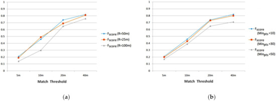
Figure 13.
Detection with different cluster algorithm settings; (a) using different cluster radius thresholds; (b) using different cluster-points thresholds.
4.3.3. Sensitivity to Data Volume
Finally, we tested the proposed method’s sensitivity to input data volume, as shown in Figure 14. We diminished the cluster-points threshold, according to the data volume. Even when only using 1/5 of the data (i.e., the subset of Shenzhen dataset), the detection quality remained stable. By adopting a re-sampling technique, our method can process massive trajectory data in a shorter time. Additionally, we noticed that detection precision dropped as we inputted more GPS points. By using more GPS points the clustering algorithm yielded increasing detected road intersections, reaching roughly twice as many as the ground truths at most. Even though we applied a road intersection classifier, the amount of false detection grew faster than the amount of correct detection, resulting in a drop in detection precision. Still, using more data can achieve better coverage of road intersections and overall performance.
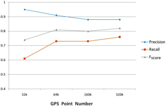
Figure 14.
Detection quality using different numbers of GPS points.
5. Conclusions
Road intersection detection is a key problem in map generation. However, low-frequency trajectories are ubiquitous among feasible GPS trajectory datasets, causing information loss which makes it hard to automatically detect road intersections. In this paper, we extended a point clustering-based method framework to detect road intersections from low-frequency data. The proposed method first utilizes geometric and hot area features of road intersections to center selected turn-points on the actual turning positions. A novel turn-point position compensation algorithm was proposed, in which false turn-points are ruled out from being compensated. Using refined turn-points and a loose threshold, the clustering algorithm obtains a recall-focused detection result, and the extended classification course can cover as many existing road intersections as possible. Next, a thinning algorithm-based binary classifier was proposed, which requires no training and, thus, is easy to implement. We found that the road intersection classification method collaborates well with recall-focused detection algorithms, offering a divide-and-conquer strategy to address the difficulty of determining a density threshold in the clustering algorithm due to the problem of high disparity in trajectory data. Moreover, the extended classification course makes our approach stable regarding parameter settings and data volume.
In summary, the proposed method represents a considerable improvement in detection recall rate and overall performance, better supporting automatic map generation and other similar applications. However, our method lacks the ability to handle complicated road intersection structures, such as highways and roundabouts. Moreover, there is ample room for further improvements in the road intersection classification algorithm. Therefore, future research will be focused on introducing a better road intersection model and mining semantic information in trajectory data, such as turning restrictions. Additionally, the binary road intersection classifier needs to be improved and extended to include type information of road intersection in the classification result.
Author Contributions
Conceptualization, Banqiao Chen, Chibiao Ding and Wenjuan Ren; Methodology, Banqiao Chen and Chibiao Ding; Software, Banqiao Chen; Validation, Banqiao Chen; Formal Analysis, Banqiao Chen; Investigation, Banqiao Chen; Resources, Guangluan Xu; Data Curation, Banqiao Chen; Writing—Original Draft Preparation, Banqiao Chen; Writing—Review and Editing, Chibiao Ding and Wenjuan Ren; Visualization, Banqiao Chen; Supervision, Chibiao Ding; Project Administration, Guangluan Xu. All authors have read and agreed to the published version of the manuscript.
Funding
This research received no external funding.
Acknowledgments
We would like to thank Assistant Prof. Desheng Zhang at Rutgers University for releasing the Shenzhen trajectory dataset. We express our thanks to the editors and anonymous reviewers for constructive comments.
Conflicts of Interest
The authors declare no conflict of interest.
References
- TomTom Map Update Service. Available online: www.tomtom.com/en_gb/maps/map-update-service/ (accessed on 22 July 2011).
- Wang, W.; Yang, N.; Zhang, Y.; Wang, F.; Cao, T.; Eklund, P. A review of road extraction from remote sensing images. J. Traffic Transp. Eng. Engl. Ed. 2016, 3, 271–282. [Google Scholar] [CrossRef]
- Mena, J. State of the art on automatic road extraction for GIS update: A novel classification. Pattern Recognit. Lett. 2003, 24, 3037–3058. [Google Scholar] [CrossRef]
- Guan, H.; Li, J.; Cao, S.; Yu, Y. Use of mobile LiDAR in road information inventory: A review. Int. J. Image Data Fusion 2016, 7, 219–242. [Google Scholar] [CrossRef]
- Goodchild, M.F. Citizens as voluntary sensors: Spatial data infrastructure in the world of web 2.0. Int. J. Spatial Data Infrastruct. Res. 2007, 2, 24–32. [Google Scholar]
- Ahmed, M.; Karagiorgou, S.; Pfoser, D.; Wenk, C. A comparison and evaluation of map construction algorithms using vehicle tracking data. GeoInformatica 2014, 19, 601–632. [Google Scholar] [CrossRef]
- Available online: https://www.cs.rutgers.edu/~dz220/data.html (accessed on 22 October 2018).
- Edelkamp, S.; Schrödl, S. Route Planning and Map Inference with Global Positioning Traces. Comput. Vis. 2003, 2598, 128–151. [Google Scholar]
- Peng, C.; Jin, X.; Wong, K.C.; Shi, M.; Liò, P. Collective human mobility pattern from taxi trips in urban area. PLoS ONE 2012, 7, e34487. [Google Scholar]
- Deng, M.; Huang, J.; Zhang, Y.; Liu, H.; Tang, L.; Tang, J.; Yang, X. Generating urban road intersection models from low-frequency GPS trajectory data. Int. J. Geogr. Inf. Sci. 2018, 32, 1–25. [Google Scholar] [CrossRef]
- Chen, C.; Lu, C.; Huang, Q.; Yang, Q.; Gunopulos, D.; Guibas, L. City-Scale Map Creation and Updating using GPS Collections. In Proceedings of the 22nd ACM SIGKDD International Conference on Knowledge Discovery and Data Mining–KDD ’16, San Francisco, CA, USA, 13–17 August 2016; pp. 1465–1474. [Google Scholar]
- Zhang, C.; Xiang, L.; Li, S.; Wang, D. An Intersection-First Approach for Road Network Generation from Crowd-Sourced Vehicle Trajectories. ISPRS Int. J. Geo Inf. 2019, 8, 473. [Google Scholar] [CrossRef]
- Karagiorgou, S.; Pfoser, D. On vehicle tracking data-based road network generation. In Proceedings of the 20th International Conference on Intelligent User Interfaces Companion–IUI Companion ’15, Lyon, France, 16–20 April 2012; p. 89. [Google Scholar]
- Wu, J.; Zhu, Y.; Ku, T.; Wang, L. Detecting Road Intersections from Coarse-gained GPS Traces Based on Clustering. J. Comput. 2013, 8, 2959–2965. [Google Scholar] [CrossRef]
- Schroedl, S.; Wagstaff, K.L.; Rogers, S.; Langley, P.; Wilson, C. Mining GPS Traces for Map Refinement. Data Min. Knowl. Discov. 2004, 9, 59–87. [Google Scholar] [CrossRef]
- Ahmed, M.; Wenk, C. Constructing Street Networks from GPS Trajectories. In Algorithms–ESA2012; Springer: Berlin/Heidelberg, Germany, 2012; pp. 60–71. [Google Scholar]
- Fathi, A.; Krumm, J. Detecting Road Intersections from GPS Traces. In Geographic Information Science; Springer: Berlin/Heidelberg, Germany, 2010; pp. 56–69. [Google Scholar]
- Xie, X.; Liao, W.; Aghajan, H.; Veelaert, P.; Philips, W. Detecting Road Intersections from GPS Traces Using Longest Common Subsequence Algorithm. ISPRS Int. J. Geo Inf. 2016, 6, 1. [Google Scholar] [CrossRef]
- Zhang, L.; Thiemann, F.; Sester, M. Integration of GPS traces with road map. In Proceedings of the Second International Workshop on Data-Aware Distributed Computing–DADC ’09, Munich, Germany, 9 June 2010; pp. 17–22. [Google Scholar]
- Li, Q.; Zheng, Y.; Xie, X.; Chen, Y.; Liu, W.; Ma, W.-Y. Mining user similarity based on location history. In Proceedings of the 16th ACM SIGSPATIAL International Conference, Irvine, CA, USA, 5–7 November 2008; p. 1. [Google Scholar]
- OpenStreetMap. Available online: http://www.openstreetmap.org/ (accessed on 22 October 2018).
- Biagioni, J.; Eriksson, J. Map inference in the face of noise and disparity. In Proceedings of the 20th International Conference on Intelligent User Interfaces Companion–IUI Companion ’15, Lyon, France, 16–20 April 2012; pp. 79–88. [Google Scholar]
- Yang, X.; Cui, W. A Novel Spatial Clustering Algorithm Based on Delaunay Triangulation. J. Softw. Eng. Appl. 2010, 3, 141–149. [Google Scholar] [CrossRef]
- Zhang, T.Y.; Suen, C.Y. A fast parallel algorithm for thinning digital patterns. Commun. ACM 1984, 27, 236–239. [Google Scholar] [CrossRef]
- Zhang, D.; Zhao, J.; Zhang, F.; He, T. UrbanCPS: A cyber-physical system based on multi-source big infrastructure data for heterogeneous model integration. In Proceedings of the ACM/IEEE 6th International Conference on Cyber-Physical Systems (ICCPS’15), Seattle, WA, USA, 14–16 April 2015; pp. 238–247. [Google Scholar]


© 2020 by the authors. Licensee MDPI, Basel, Switzerland. This article is an open access article distributed under the terms and conditions of the Creative Commons Attribution (CC BY) license (http://creativecommons.org/licenses/by/4.0/).