Article

Accuracy Assessment of a UAV Block by Different Software Packages, Processing Schemes and Validation Strategies

by
Vittorio Casella
1,
Filiberto Chiabrando
2,
Marica Franzini
1,* and
Ambrogio Maria Manzino
3
1
Department of Civil Engineering and Architecture, University of Pavia, Via Ferrata, 3, 27100 Pavia, Italy
2
Department of Architecture and Design, Polytechnic of Turin, Viale Pier Andrea Mattioli, 39, 10125 Turin, Italy
3
Department of Environment, Land and Infrastructure Engineering, Polytechnic of Turin, Corso Duca degli Abruzzi, 24, 10129 Turin, Italy
*
Author to whom correspondence should be addressed.
ISPRS Int. J. Geo-Inf. 2020, 9(3), 164; https://doi.org/10.3390/ijgi9030164
Submission received: 31 January 2020 / Revised: 14 February 2020 / Accepted: 8 March 2020 / Published: 11 March 2020
(This article belongs to the Special Issue Enhanced Modeling and Surveying Tools for Smart Cities)

Abstract

:
Unmanned aerial vehicle (UAV) systems are heavily adopted nowadays to collect high-resolution imagery with the purpose of documenting and mapping environment and cultural heritage. Such data are currently processed by programs based on the Structure from Motion (SfM) concept, coming from the computer vision community, rather than from classical photogrammetry. It is interesting to check whether some widely accepted rules coming from old-fashioned photogrammetry still holds: the relation between accuracy and ground sampling distance (GSD), the ratio between the vertical and horizontal accuracy, accuracy estimated on ground control points (GCPs) vs. that estimated with check points (CPs) also in relation to their ratio and distribution. To face the envisaged aspects, the paper adopts a comparative approach, as several programs are used and numerous configurations considered. The paper illustrates the dataset adopted, the carefully tuned processing strategies and bundle block adjustment (BBA) results in terms of accuracy for both GCPs and CPs. Finally, a leave-one-out (LOO) cross-validation strategy is proposed to assess the accuracy for one of the proposed configurations. Some of the reported results were previously presented in the 5th GISTAM Conference.

1. Introduction

The use of unmanned aerial vehicles (UAVs) for surveying purposes such as mapping, 3D modeling, point cloud extraction and orthophoto generation has become a standard operation in recent years. The large availability of so-obtained 3D models force the scientific community to explore and develop new tools for visualizing and sharing the achieved products and, as a consequence, open new scenarios strictly related to the use of virtual and augmented reality that for sure need to be considered as an important research topic even more related to the geospatial information [1,2]. Within this framework, the high quality of commercial off-the-shelf cameras, easily implemented in UAV platforms and the development of new generation software packages created an important revolution in the geomatics field. Mapping and 3D modeling are increasingly exploiting UAV potentialities in several applications, many of which, as the present paper, related to morphological landscape surveying. The topographic characteristics of these sites are significantly different, since they include rivers [3,4,5], shore regions [6,7], gullies [8], pits [9,10] or glaciers [11,12]; nevertheless UAV photogrammetry has always produced satisfactory results, thanks mainly to the capability of the Structure from Motion (SfM) approach to take advantage of the high spatial resolution of images to recognize textures at the ground even for uniform surfaces [6,13].
The SfM technique operates under the same basic principle of traditional photogrammetry in which the 3D position of a point can be resolved from a series of overlapping images [14]. What differentiates SfM from conventional photogrammetry is the use of a new generation of image-matching algorithms, developed within the computer-vision community, capable to automatically extract a database of features from a set of multiple overlapping images [15]. We have then assisted to a transformation in the photogrammetric community that has adopted this new technique, demonstrating its potentiality in several contributions such as [13,16,17,18,19].
The SfM approach is particularly of great interest in the processing of images acquired by UAV, where a series of characteristics such as path irregularity and varying altitude, which produce variation in overlapping, image scale and resolution, can cause problems to the classical photogrammetric method but where SfM algorithms are instead able to recognize a very large number of homologous features [5]. This capacity is even more useful when a well-defined flight plan cannot be prepared for emergency reasons [20] or for morphological constrains [21].
In the first step, SfM aligns the imagery solving the collinearity equations in an arbitrary scaled coordinate system without any initial requirements of external information (camera location and attitude or ground control points (GCPs)). To frame the block to the ground reference system, two alternatives are possible: a seven-parameters rigid transformation or a bundle blocks adjustment. The former, simpler, can introduce significant distortions in the final 3D product if the SfM-automated matching points present not neglectable errors [5]; the latter, more complex, allows to exploit photogrammetric experience to compute external orientation parameters but also to perform camera calibration and evaluate block precision and accuracy [13]. For the second strategy, several studies deal with performance of UAV survey under several block configuration and, nowadays, when the UAV and SfM combination has led out on the photogrammetric marketplace different software solutions and also package performances; a review can be found in [22].
Block configuration influences BBA results under several point of views related to flight schema, flying height, overlapping and the number and distribution of GCPs. A correct flight configuration must be planned according to the area of interest (AOI), the required ground resolution (expressed by the ground sampling distance) and acquisition geometry [23,24]. Flying rather high with a high side overlap guarantees an optimal acquisition geometry and a ground resolution enough for most of the common medium-scale applications. For instance, [25] gives an exhaustive overview of the influence of altitude, overlap and weather conditions for a forestry survey. Several blocks were acquired at a flying height between 20 and 80 m and with a side overlap range of 20% to 80%. Optimal configuration is reached with a side overlap at least of 60% and a flying height of about 80 m. Some examples of similar conclusions can be found in [26] for landslide monitoring purposes, in [27] for olive orchards, who suggest also a high forward overlap (95%) and in [28], which analyze the influence of highly overlapping imagery in a 3D point cloud generation for a large test site of about 40 ha. Number and distribution of GCPs have been explored by several authors too. In [29], the influence of six different GCP configurations (from a minimum of 4 to a maximum of 9 GCPs, located only on the block edges or also in the central area) have been studied for digital orthophoto and digital elevation model (DEM) production, using a fixed-wings UAV in Malaysia. Besides, [19] evaluated the influence of GCP numbers and distributions in terms of DEM quality for two case studies located in Morocco and France, while [30] have conducted a similar experience to produce a multispectral orthomosaic for crop management; in this case, the main key factor was represented by the spatial distribution of the GCPs. Finally, [31] evaluates the horizontal and vertical accuracy for 13 cases of GCP configurations. Generalizing the results, it is confirmed that a small number of GCPs is useful only when data transformation (seven-parameters rigid transformation) is required while a larger number is necessary for camera self-calibration. For the second aim, spatial distribution is important too, as ground points should cover the whole AOI. Precisely because only a large GCPs number is useful for the stabilization of interior orientation, it is necessary to evaluate different approaches based on more accurate camera distortion models and, at the same time, on a reduction of markers number. However, since complex distortion models can over-parameterize the system, an independent ground control becomes mandatory, and the leave-one-out (LOO) cross-validation method can be applied to evaluate it. LOO is a statistical estimation technique where the original data are partitioned in k-training subsets of equal size; the overall accuracy is obtained averaging the accuracy values computed on each subset. This method, originally applied in other fields like machine learning [32], is more recently adopted in geomatics applications such as accuracy assessment of satellite imagery orientation [33] or as outliers’ detector for least squares compensation in geodesy [34].
After establishing the ideal configuration, software solutions performance must be evaluated too. In [35], five software packages (Microsoft Photosynth - University of Washington, USA, Bundler - University of Washington, USA, PMVS2 – University of Illinois, USA, Agisoft PhotoScan - St. Petersburg, Russia and ARC3d – Ku Leuven, Belgium) are compared for 3D point cloud generation, and results are strongly influenced by the program choice in terms of point density, distribution and accuracy. Additionally, in [36], five software packages are compared, some of which not based on the SfM approach: Erdas-LPS – Heerbrugg, Switzerland, EyeDea -University of Parma, Parma, Italy, PhotoScan, Pix4D – Prilly, Switzerland and PhotoModeler – Vancouver, Canada. Even if the SfM software can provide results in an automatic way (the photogrammetric ones have required an operator intervention in some phases), they present worst results in terms of the root mean square error (RMSE) of control points. Besides, [21] compares the geometric accuracy of the DSM (digital surface model) computed using different scenarios, number of images and GCPs and two software packages: PhotoScan and IGN MicMac – Saint-Mandè, France. Both software packages provide satisfying results, even if PhotoScan seems to provide better results (limited deviation in the DSM and better reconstruction) outside the control region (GCPs’ bounding box). Other examples can be found in [37,38,39,40,41].
Starting from these assumptions, the aim of the paper is to analyze the performance of five software packages which are today generally employed for processing the data acquired by UAVs using the SfM-oriented approach. The work deals with the data acquired by a UAV flight performed over a sandpit where several points were measured to use within the BBA operation to perform an independent check afterwards. The different followed strategies are accurately described in terms of weights of the observations used in the adjustment, strategies for tie point extraction and number of GCPs and check points (CPs). Besides, an accurate analysis of the achieved results is reported to understand which are the problems that could be founded during the data-processing and which strategy should be the most suitable for the survey purpose. Finally, the LOO cross-validation method is adopted to assess the block accuracy for one of the proposed configurations.

2. Methods

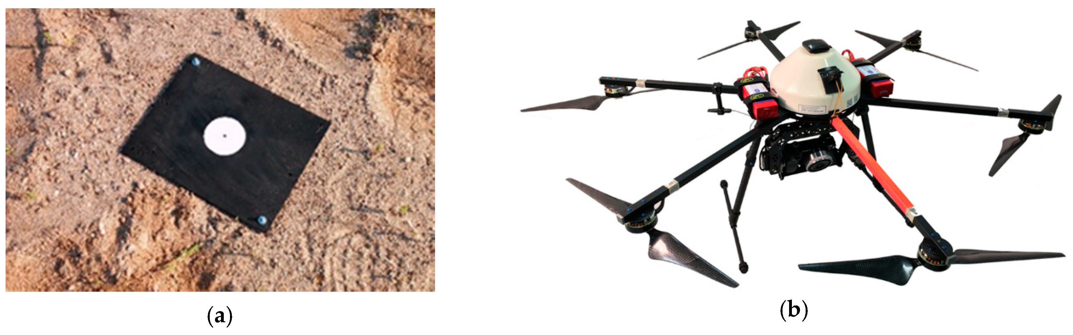
2.1. Data Acquisition

The test site is a part of a large sandpit located in the Province of Pavia, in Northern Italy (Figure 1a). The selected area roughly has a horseshoe configuration and is constituted by two flat regions connected by the excavation front, being 10 meters high and having a slope between 30° and 90°. The upper flat zone and the scarp are mainly bare, while the lower one shows a large vegetated area (Figure 1b). The surveyed surface is approximal 2 hectares.
Before the flights, 18 markers (Figure 2a) were positioned and surveyed by an integrated use of a total station (TS) and a GNSS receiver. The GCPs’ proper names range from CV1 to CV18 and are constituted by a black wooden plate with a white painted circle having a diameter of 8 cm. The markers were surveyed with the TS in a redundant way; that means that each of them was observed from different stations, and their relative coordinates were obtained by a least-squares adjustment (data were processed with MicroSurvey Star*Net). Moreover, some stations were also measured with GNSS in order to orient the whole survey in a map reference system. Final precision is around 0.5 cm for the horizontal components and 1 cm for vertical one. This was not a conventional approach for markers measurements, since it is usually be surveyed via the real-time kinematic (RTK) GNSS technique, but this choice would have introduced an uncertainty of some centimeters in their positions (between 2–4 cm in the horizontal component and 3–5 cm in the vertical one). These values are, in our opinion, too high for the considered UAV blocks that have a ground resolution less than 2 cm; for this reason, a more accurate topographic survey was performed.
Several photogrammetric blocks were acquired by a UAV equipped with a Sony A6000 camera (Figure 2b) under different configurations. The vehicle was made by a small Italian company named Restart® and has the following main characteristics: 6 engines (290W each one), Arducopter-compliant flight controller, maximum payload of 1.5 kg (partly used by the gimbal, weighting 0.3 kg) and flight autonomy of approximately 15 min.
The camera has a 24 MP sensor and a focal length of 16 mm (Sony lens E16mm F2.8 Wide Angle). Ground resolution is 17.5 mm at the 70 m above ground level (AGL), and about 10 mm at 40-m AGL. The quality of the markers ground coordinates was then suitable for both flying heights. The blocks acquired over the area are all listed in Table 1: they can subdivide into two main sets according to their flying heights, 70 m and 40 m; moreover, inside each of them, both nadiral and oblique imagery were taken. Block 5 was flown looking toward the scarp, following a circular trajectory, and with a bit lower altitude—30 m instead of 40—to insure the same ground resolution of blocks 6 and 7. The present paper only concerns a dataset coming from the union of blocks 1 and 2, constituted by seven strips (Figure 3a) and 82 images; end lap (longitudinal) and side lap (lateral) were 77% and 60%, respectively (more details can be found in [42]). The authors have selected these two blocks for the presented analysis, because they were acquired at a quite common configuration in terms of flying height and geometry (grid), allowing to potentially extend the obtained results (Section 3) to a wide range of case study; the two blocks were jointly processed. The other acquired blocks will be investigated in further analysis, as reported in Section 4.

2.2. Data-Processing

The University of Pavia and the Polytechnic of Turin decided to process the same dataset with different software packages they are experts on. The Pavia unit used Agisoft PhotoScan (now named MetaShape) and Inpho UAS Master (Sunnyvale, USA), while, in Turin, Pix4D, ContextCapture by Bentley Systems (Exton, USA) and MicMac were used. GCP/CP configurations were discussed in advance and kept fixed by both groups. Three scenarios were considered, shown by Figure 3b–d, according to the criteria listed below; GCPs are shown in red and CPs in blue:
  • Configuration 1—all the markers are used as GCPs, to perform robust camera calibration (18 GCPs/0 CPs);
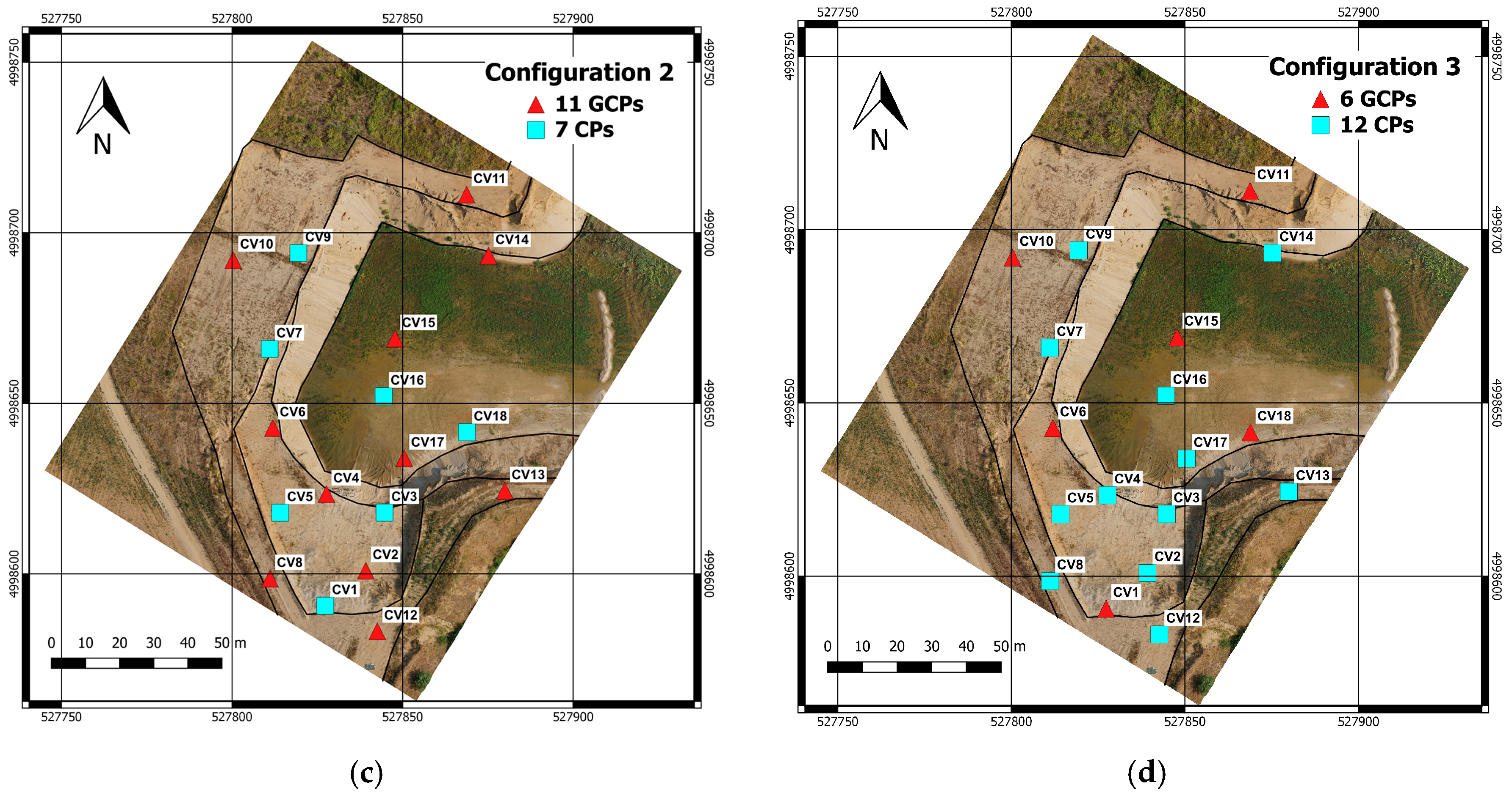
  • Configuration 2—an intermediate setup with strong ground control and still some check points (11 GCPs/7 CPs);
  • Configuration 3—only six points are used as GCPs, that is realistic for routine surveying (6 GCPs/12 CPs).
The three configurations faced different issues. Configuration 1 is characterized by the presence of several GCPs that are mandatory to perform a robust camera calibration, as reported in [29]. For this reason, this configuration was mainly used to tune how many and which inner camera parameters must be optimized. This output guided the camera recalibration settings of the further two configurations, which had instead the main goal of evaluating the influence of ground control on the final accuracy.
The workflow followed by the five programs was similar and composed by image alignment, GCPs measurement, BBA settings in term of camera self-calibration and weighting strategies of the observations. In the next sections, the settings adopted for each of them are reported in order to provide all the information useful to understand the choices that led to the reported results. Once the BBA was run, residuals for GCPs and CPs were evaluated, as reported in Section 3; further stages, such as dense point cloud generation or orthomosaic production, were not taken into consideration outside the purposes of this paper.

2.2.1. Agisoft PhotoScan

The first software package tested was PhotoScan (rel. 1.2.4) developed by Agisoft LLC (St. Peterburg, Russia) [43]. Once images are loaded into the program, they need to be aligned, which means that, for each photo, approximate camera position and orientation are computed and tie-points are extracted in the form of a sparse point cloud. For the photo alignment, the “high accuracy” setup was chosen, in which tie points were extracted from the full-resolution images, while the “pair preselection” parameter was set on “generic”, since no a priori information about imagery positions was available. If camera positions would be available, for instance, thanks to a GNSS on-board receiver, they could be used at this stage; our dataset did not have this kind of information. The initial alignment was carried out with only the support of SfM algorithms. GCPs were then measured on the imagery in a cautious way; meaning that, for each image, only clearly visible points were measured. This means that markers partially covered by obstructions or excessively deformed due to their proximity to image borders were discarded. The average number of measurements per marker was 15, with a minimum of 9 for CV7 and a maximum of 29 for CV17. It is important to specify that GCP measurements were performed only one time, and the same collimations were used for all the three configurations (this procedure was followed for all the five software packages).
The third and fundamental key step is the BBA settings in terms of camera self-calibration and weighting strategy. Concerning the former, after some testing conducted on Configuration 1, it was decided to adopt the parameter set proposed as a default by the program. It is constituted by the focal length (f); the corrections for the principal point position (cx and cy); the first three coefficients of radial distortion (K1, K2 and K3) and the first two of tangential distortion (P1 and P2). We did not insert any approximate values for the camera model, as that did not apparently give any benefit. It is important to point out that PhotoScan is particularly flexible from this point of view, because it allows to select the single parameters that must be optimized. Weighting strategy refers to the precision that must be ascribed to the observations inserted in the adjustment that are, in our case, are constituted by two categories: object coordinates of GCPs and image coordinates of GCPs and tie-points. Accuracy of ground coordinates of markers was set at 0.5 cm for the horizontal component and 1 cm for vertical one, which are the values obtained from the topographic adjustment. For the manually measured image coordinates of the markers, accuracy was set at ¼ of the pixel size, while for automatically measured image coordinates of tie-points, accuracy was set at 1.5 pixels, corresponding to three-times the overall reprojection error. In doing so, we followed the suggestions of the program developers, to be adopted in the case of blurred images; we also verified that the implemented strategy gave the best results in terms of residuals for the CPs.

2.2.2. Inpho UAS Master

Inpho UAS Master (rel. 7.0.1) is a photogrammetric suite sold by Trimble (Sunnyvale, USA). Processing steps and settings are like those described for PhotoScan, even if there are a couple of differences. The first and main is that UAS Master requires the knowledge of approximate external orientation parameters to extract tie-points. Since our dataset does not have such information, the orientation values coming from PhotoScan were used; this choice has only been motivated by the fact that both programs were managed by Pavia’s unit (information obtained by one of the other software packages could be used equally). This, which could look like a big limitation, is progressively losing its relevance thanks to the spreading of on-board GNSS receivers capable to supply the approximate locations.
Once provided these values, tie-point extraction was performed using the “full-resolution” mode. GCPs were measured by a different operator, with the same style of being cautious and measuring only well-visible targets; the mean number of observations was 15, with a minimum of 9 measurements on CV8 and a maximum of 26 on CV17. Camera self-calibration was performed using Configuration 1 results as reference points, and the parameters adopted are the same of PhotoScan. Weighted strategy is instead a little different, because UAS Master does not allow to set the uncertainty of image coordinates of markers and tie-points; we infer that the program applies default values. Object coordinates of markers were weighted as illustrated above, using the values obtained from the topographic adjustment.

2.2.3. Pix4D

Pix4D (rel. 2.1.61) is a well-known software package developed by a Swiss company started in 2011 as a spinoff of the École Polytechnique Fédérale de Lausanne (Prilly, Switzerland) [44]. To perform the initial stage of image alignment, several parameters must be set. About key point extractions, the “full” option was set, meaning that imagery was used at the full resolution; besides, according to the input data, the matching was set up for “aerial grid”. The program requires immediate information on processing strategy; the number of the key points was set to “automatic”, while the calibration method to “standard”. The last choice refers to the initial optimization of all the internal parameters: since it is well-known that the cameras used with UAVs are much more sensitive to temperature or vibrations, which affect the camera calibration, it is recommended to select this option when processing images taken with such cameras. GCP measurements were carried out according to the strategy previously reported; in this case, the average number of measurements per marker was 26, with a minimum of 15 for CV10 and a maximum of 40 for CV17.
Last step was the BBA, in which the camera self-calibration is calculated using the default option, which is related to the focal length (f); the corrections to the principal point position (cx and cy); the first three coefficients of radial distortion (K1, K2 and K3, called R1, R2 and R3 in Pix4d) and the first two of tangential distortion (P1 and P2, called T1 and T2 in Pix4d). About the weighted strategy, GCP object coordinates were set according to the accuracy obtained by topographic survey (0.5 cm for horizontal components, while the vertical one was fixed at 1 cm). It is not possible in Pix4D to set the accuracy of the measurement on the images, probably this value as commonly used is fixed by default at ½ of the pixel size.

2.2.4. Bentley ContextCapture

The fourth employed commercial software package was ContextCapture (4.3.0.507) by the Bentley Systems (Exton, USA). The strategy followed by this program is like the ones described above. The initial alignment was performed using the default setting with “high” density in the key point extraction (scale image size); in this first step, the software starting from the information derived by the EXIF file adjusted the camera internal parameters as well (f, cx, cy, K1, K2, K3, P1 and P2). EXIF information was only used as initial approximate values, as it is well-known that its quality is not adequate for photogrammetric purposes [45]. After the first processing step, the camera pose was estimated in an arbitrary coordinate system; the next step was the GCP measurements. In order to help the operator in the measurement phase, this part was performed first using three GCPs in three different images, and then a rigid registration was performed. Starting from these first results, an accurate measurement of the other points was achieved; the average number of measurements per marker was 15, with a minimum of 9 for CV10 and a maximum of 33 for CV17. Finally, the BBA weighting for the two components of GCP object coordinates was set according to the other programs, since it was not allowed to set the accuracy of the GCPs and key-point image coordinates. Camera optimization was performed as well to define the internal parameters of the employed camera.

2.2.5. MicMac

Furthermore, according to the actual trend in the geospatial information area, which put even more attention on the open-source software and tools in the presented test, the open-source software MicMac was employed. The software has been developed by the MATIS laboratory (IGN, Saint-Mandè, France), and it has been delivered as an opensource in 2007, usable in different contexts (satellite, aerial and terrestrial) for extracting point clouds from images [46]. The pipeline of the software [47] is quite different compared to the commercial one, since all the commands in the employed version (5348 for Ubuntu) need to be inserted by the terminal.
The first used tool was Tapioca, with this command MicMac computing the tie-points on the images. The options that could be used in Tapioca were the strategy for extracting the information from the images (All, MulScale, etc.) and the number of pixels that we need to use for extracting the tie-points. In the present test, all the possible pairs were analyzed (option All) with the use of the full-image resolution (option 1 in MicMac) in order to extract the maximum number of tie-points. This choice was very time-consuming but allowed to better evaluate the internal parameters when the use of a more complex calibration model was needed. After Tapioca, only the tie-points were extracted, to align the images according to the extracted points another tool needs to be launched: Tapas. This command allowed to calibrate the images and to align them in a local reference system according to several parameters. According to the previous tests reported in [48], in order to improve the achieved results after the bundle block adjustment, a more complex calibration model was used. The employed calibration model was the one reported in [49], hereafter called F15P7. This model was developed for reducing the so-called “bowl effect”, adding additional degrees to the radial correction. More in-depth, first a basic model was calculated ([49] or other models); furthermore, using the first model as an initial value, extra polynomial coefficients were added to improve the description of the optical deformations, and finally, a nonradial polynomial correction was added to rectify the deformations left. The step-to-step approach was carried out in order to limit the risk of over-parametrization, a factor that was also controlled according to the large amount of GCPs employed in the present test.
The next step was the image-point measurements. This part was performed in two steps using an approach like the one used in ContextCapture: first, using three GCPs in three different images, a rigid registration was performed (using SaisieAppuisInit for image measurements and GCPBascule for the rigid registration). Starting from these first results, an accurate measurement of the other points was achieved (SaisieAppuisPredict); the average number of measurements per marker was 18, with a minimum of 14 for CV10 and a maximum of 36 for CV17.
Finally, for performing the BBA, the weighting factor for the two components was fixed at 1 cm (it is not possible in MicMac to adopt different weights for the horizontal and vertical components). For the image coordinates of the manually measured markers, the accuracy was set at ½ of the pixel size. During the BBA in MicMac (Campari), c as the initial interior calibration parameters—the ones derived from the first orientation process—were used (carried out using Tapioca). Furthermore, during the adjustment, the calibration was reoptimized setting the option AllFree in order to re-estimate the different parameters using the GCPs3 bundle block adjustment results.

3. Bundle Block Adjustment Results Analysis

3.1. GCPs and CPs Residuals Analysis

The quality of aerial triangulation was evaluated by assessing the differences between the photogrammetrically measured object coordinates of GCPs and CPs and the ground-surveyed ones.
Table 2, Table 3 and Table 4 group results per configuration. Table 2 shows, for instance, results concerning GCPs and CPs for all the programs considered only for Configuration 1. We show the name of the software used, the mean, standard deviation and RMSE values of the differences between the photogrammetrically obtained object coordinates of markers and those determined by surveying; the analysis was performed for all the X, Y and Z components of the GCPs and CPs, if any. Tables illustrating the behavior of the same software package through the configurations depicted are reported in Supplementary Materials (Tables S1–S5).
Figure 4 graphically summarizes results for the three configurations and five programs in terms of the RMSE. The ground sampling distance (GSD) for the considered imagery is around 1.8 cm and is represented with a red dashed line in the figures. RMSE values are almost always below the GSD values, thus highlighting that results are good in general. In Configuration 1, RMSE figures are all below the GSD threshold for all the components and the programs adopted. Configuration 2 shows similar results also for the vertical component, with an exception for the UAS Master, which is slightly above it. In Configuration 3, all RMSE figures are within the GSD threshold apart from the Z component for ContextCapture (for both GCPs and CPs) and the Z of the CPs for the UAS Master. Figure 4 suggests that results for the various packages are comparable to a first approximation, and, to adequately support this statement, further analysis has been performed in Section 3.2.
However, before moving to this comparative analysis, a deeper residual assessment was conducted, analyzing them graphically. Figure 5 and Figure 6 illustrate the residuals for only Configuration 3, because it shows the largest differences between the five programs (figures for the other two configurations are reported in the Supplementary Materials, Figures S1–S5). All the 18 markers are reported: GCPs are represented by triangles, whereas CPs are squares. Red segments show horizontal residuals; they originate from their true position, which was determined by ground surveying, and end where photogrammetric measurements locate them. Vertical residuals are represented by blue vertical segments. In order to make them visible, all the residuals were magnified, and a ruler is shown in the lower right part of each picture corresponding to 1 cm. The scale ratio is the same for each figure in order to favor comparisons.
In the lower part of the test site, where markers are more numerous, the residuals show different behaviors between the software packages. Unfortunately, GCP locations are not uniform, because some constrains, such as the presence of swampy terrain, have led to this final distribution (which is, in any case, representative of a real case, where is not always possible to put the markers in an optimal configuration). Focusing on the CP vertical component, Pix4D and MicMac present small residuals, while the others three show larger values; more interesting, the directions of these residuals are often opposite. The source of this diversity could be researched in different software behaviors, connected, for instance, to the quality of the extracted tie-points or in a weakness of the ground control, which can influence the results. To deal with this issue, a cross-validation analysis is proposed in the Section 3.3.

3.2. Comparative Analysis Among Software Packages

As previously reported, Figure 4 suggests that results for the various packages are comparable at a first approximation. Considering, as an example, the RMSE for X components of GCP residuals in Configuration 1 (Table 2); we report them here for maximum clarity: 0.003, 0.002, 0.004, 0.004 and 0.004. We tried to answer the following question: Can we assume they are extractions from the same random variable? To properly motivate the answer, confidence intervals have been calculated, having 95% probability, following the well-known formula about the probabilistic distribution of the sample variance s 2 :
( n 1 ) S 2 σ 2   ~ χ n 1 2
Equation (1) can be used to derive confidence intervals such as:
χ n 1 ; α / 2 2 σ 2 n 1 s 2 χ n 1 ; 1 α 2 2 σ 2 n 1      P = 1 α
where χ n 1 ; α / 2 2 and χ n 1 ; 1 α 2 2 are two values characterized by
P ( χ n 1 2 χ n 1 ; α 2 2 ) = α / 2 P ( χ n 1 2 χ n 1 ; 1 α 2 2 ) = α / 2
For each obtained RMSE, the average value of the standard deviation has been calculated. For our example, the first GCP coordinate for Configuration 1, this value is 0.0034, and it was used as the value of σ in the above-reported formulas. Within them, n is the number of the residuals used to estimate it, and, in this case, n = 18 . The confidence interval was calculated, and single variance determinations were tested. The analysis found that there are some borderline values and two proper outliers represented by the Z component of ContextCapture in Configuration 3 (Table S6 in the Supplementary Materials summarizes the analysis).
Statistical testing confirmed that results from various packages are comparable. Therefore, it was decided to synthetize the results that are reported in Table 5. Two cells contain two values: the upper one is obtained as explained above; the lower one is calculated excluding two anomalous values shown by ContextCapture. To keep the following discussion reasonably simple, the second figure will only be considered.
Values reported in Table 5 suggest several remarks. First, results confirm the well-established photogrammetric rule for which horizontal components perform better than Z. The average value is 0.005 m for the horizontal figures and 0.013 m for the vertical one (and decreases to 0.011 m when two anomalous figures are omitted, corresponding to the Z RMSE of ContextCapture for Scenario 3). Besides, RMSE values are lower for GCPs than for CPs. Overall average values for GCP/CP are 0.005/0.011 m. For the sole horizontal components, results are 0.004/0.006 m, while, for the vertical one, we have 0.009/0.015 m; the increase factor is slightly higher for altimetry than for planimetry.
One gold rule of photogrammetry (and of the treatment of observations in general) is that the use of independent information is recommended to properly validate the results of adjustments. In traditional photogrammetry, where there are 10 to 20 TPs (tie-points) per image, the use of a significant number of CPs is recommendable, as statistics on GCPs has little or marginal significance. Our paper highlights instead that, in SfM photogrammetry, statistics on GCPs are comparable to that on CPs, though lower. Concerning the different configurations, RMSEs for GCPs are weakly influenced by their numerosity. For the first two scenarios, they show the same overall mean value: 0.005 m. In the third configuration, values become more irregular and increase. Irregularity is more visible for the Z component and is probably due to variability of the estimators, which are caused in turn by the few degrees of freedom; it also is highlighted by the extreme value of 0.001 m for X in PhotoScan. Overall mean for the third scenario is 0.008 m; if two extreme values are discarded (the one already mentioned and the Z value for ContextCapture, being 0.028 m), the average is 0.007 m. UAS Master and ContextCapture show Z values higher than the other programs. RMSEs for CPs are weakly influenced by point numerosity for X and Y and, more significantly, for Z. Discussion here is obviously limited to Scenarios 2 and 3. Overall mean values for X and Y are the same: 0.006 m. For Z, we have 0.013 m for Scenario 2 and 0.021 m for the third one (if ContextCapture is excluded, the latter figure becomes 0.009 m and 0.016 m).

3.3. Cross-Validation

Leave-one-out (LOO) cross-validation is a statistical estimation technique that uses a single observation as a test between all those used for parameter calculations. This observation, left outside the adjustment, changes from time to time within the n-considered ones. In our case, the set of observations is constituted by the GCPs, and, at each iteration, one of them is left outside the BBA, becoming a CP. The residuals’ set obtained on this single point at each stage can be used for statistical analyses, like mean, median or standard deviation calculations.
This well-known method is not largely applied in the photogrammetric field yet. However, an example can be found in [50], where a wide test site in Spain was surveyed by UAV, and more than 100 targets were placed and measured with a GNSS receiver. In this experience, the final goal was the assessment of the influence of the GCPs’ numerosity and the location of the block accuracy; the method was implemented with several configurations in which the dimensions of the left-out subset from the BBA progressively increased.
In our paper, LOO was used to assess the quality of the GCPs. As previously discussed at the end of Section 3.1, the residual CPs, for Configuration 3, show different behaviors among the tested programs. This phenomenon could be connected to a weakness of the ground control, and a cross-validation analysis can support this analysis.
LOO validation was applied for two software packages: PhotoScan and MicMac and one configuration: Configuration 1. The choice of the software packages was motivated by the necessity to use programs with good performances (both have overall optimal results) but having different behavior in terms of residuals (compare Figure 5a and Figure 6b). As the analyzed phenomenon could be connected also to a lack in the data-processing, using programs with overall good results are important. The use of Configuration 1 was instead necessary to have a strong ground control; in our test site, where GCPs are not uniformly distributed, the use of Configurations 2 or 3 for such analyses could have distorted the results. The option to leave more markers out was not feasible due to their lack in the northern area.
Following the same settings established for the traditional accuracy assessment (see Section 2.2.1 and Section 2.2.5 for more details), the bundle block adjustments were iteratively performed, leaving each time a GCP out. Since Configuration 1 has 18 GCPs, 18 iterations were executed (computational cost is minimal, since the method requires only BBA reiteration), and, for each of them, the excluded marker was considered as the CP, and differences with ground-surveyed object coordinates were formed. Table 6 shows, for the two tested software packages, the final statistics; since these residuals can be considered as independent extractions from the same random variable, the main statistical figures can be produced.
Figure 7 reports graphically the residuals obtained for each marker. For better comprehension, each figure shows with black lines the main terrain features together with the 18 GCPs. Red segments show horizontal residuals; they originate from their true position, which was determined by ground surveying, and end where the photogrammetric measurements locate them. Whereas, vertical residuals are represented by blue vertical segments. One again, in order to make them visible, all the residuals were magnified, and a ruler is shown in the lower right part of each picture corresponding to 1 cm.
Our hypothesis is that, when the quality of a photogrammetric block must be evaluated, the LOO method can be considered a good technique, allowing to analyze how each single GCP influences the results and if, among them, some outliers are present. The obtained residuals do not show anomalies in any points. This means that the behavior discussed in the previous section depends on software packages instead on ground control quality; the residuals observed in the lower test site area could be connected to differences in the tie-point extractions. Besides, a more interesting remark can be done observing that the obtained values (Table 6) are comparable with the results obtained in terms of CPs for PhotoScan and MicMac in Table 4; the RMSE values are very similar, with discrepancies lower than 20%. This comparison seems to suggest how the LOO method can be also useful to evaluate block quality in case a few GCPs are available (in substitution of the traditional subdivision between GCPs and CPs).

4. Discussion and Further Activities

A significant part of a sandpit was surveyed by a UAV equipped with a Sony A6000 camera. A set of ground points were measured and used either for block orientation or quality assessment. Five software packages were compared: PhotoScan, UAS Master, Pix4D, ContextCapture and MicMac. They were used to perform BBA in three configurations characterized by a different ratio between GCPs and CPs. In Configuration 1, markers were all used as GCPs to perform robust camera calibration, Configuration 2 dealt with an intermediate setup with strong ground control and some check points and Configuration 3 was the more realistic one and simulated a routine surveying.
For each program, the BBA strategy was carefully studied, and final settings were tuned to optimize results. Section 3 contained an extensive discussion on the BBA parameters, since the processing choices significantly influenced the final accuracy. In literature, other authors have worked on this topic; [20] reported that appropriate camera models and tie/control points weighting can improve the results, while [36] showed that better values can be found in programs that have the capability to set the computation parameters in comparison with those that follow a black box approach. The software packages tested in the present paper have different levels of configurability: PhotoScan and MicMac (remembering that this last is an opensource project) were the most flexible programs, because they allowed to configure, contrary to the other three, whose interior parameters must be optimized or image coordinates must be weighted.
Residuals between the photogrammetrically obtained object coordinates of markers and those determined by surveying were formed and analyzed. Results for PhotoScan, Pix4D, UAS Master and MicMac were always good and comparable, less than 1 GSD for the horizontal components and less than 1.5 GSD, at worst, for the vertical one. Therefore, the decreasing number of GCPs influenced results but less than expected. The only exception was ContextCapture for the vertical component, as better discussed in the following.
The obtained accuracies were extremely good and lower than the well-accepted practical accuracy of 1−2 GSD in planimetry and 2−3 GSD in altimetry. This outcome can be attributed to the BBA strategies, optimized for the tested block, and to the high quality of the ground truth (GCPs/CPs had a precision of 0.5 cm for the horizontal components and 1 cm for the vertical one). The general trend followed that reported by other authors, such as [30], who showed as the horizontal accuracy was better than the vertical one, and both are better when the number of GCPs increased (even if only slightly). In literature are also present papers in which GCP numbers and distributions assume key roles in the final accuracy. The authors of [51] show that, to achieve optimum results in planimetry, the GCPs must be placed on the edge of the study area; besides, it is advisable to create a well-distributed configuration with a density of around 0.5–1 GCP per hectare to minimize altimetry errors; this conclusion was achieved using more than 70 markers. This outcome, even if interesting from a scientific point of view, refers to a nonrealistic routine surveying, and the question arises as to whether it can be reached also with a more traditional configuration, like that proposed by us and other authors [30,31,32]. As previously reported, the only exception is ContextCapture, which presented larger values in the vertical component for Configuration 3. This result was not an isolated case for this program, and a similar one can be found in [52]. This paper reported the accuracy of some software packages, among them, ContextCapture, in the processing of data acquired by UAVs on a coastal area. In this case study, ContextCapture performed worse than other softwares, such as PhotoScan and Pix4D, both for horizontal and vertical components. In our experience, only the altimetry suffered by the ground configuration, while planimetry obtained always good results and was comparable with the other programs. Moreover, excluding the anomalous residuals shown by ContextCapture, the values obtained by the five programs were fully comparable and can be summarized in a unique table (Table 5).
Finally, an innovative use of the leave-one-out cross-validation was proposed to assess how each single GCP influenced the results and if, among them, some outliers were present. The analysis was conducted only for the two best performer software packages: PhotoScan and MicMac but did not highlighted anomalies in any GPCs, meaning the values discussed depended only on programs instead of on ground truth quality.
Further activities will follow different directions. On one hand, the other flights described in Table 1 will be processed with attention to oblique blocks in order to investigate their influence on final accuracy. On the other, final products, such as dense point clouds, will be assessed to explore the influence of BBA parameters in their generation. Several check points (more than 250) were already measured with a topographic total station on the upper flat area and on the scarp of the sandpit. An accurate comparison between the achieved point clouds and these points will be performed; an evaluation of point density will also be realized, comparing the clouds obtained in flat or scarp areas. LOO cross-validation analysis will be also extended, taking into consideration other information such as tie-points.

5. Conclusions

A significant part of a sandpit was surveyed by a UAV equipped with a Sony A6000 camera. A set of ground points were measured and used either for block orientation or quality assessment. Five software packages were compared: PhotoScan, UAS Master, Pix4D, ContextCapture and MicMac.
Residuals between the photogrammetrically obtained object coordinates of markers and those determined by surveying were formed and analyzed. Results for PhotoScan, Pix4D, UAS Master and MicMac were always good and comparable, less than 1 GSD for the horizontal components and less than 1.5 GSD, at worst, for the vertical one. The only exception was ContextCapture which presented some outliers in vertical component; excluding these anomalous residuals, values obtained by the five programs were fully comparable. Besides, the decreasing number of GCPs influenced results but less than expected. This outcome can be attributed to the BBA strategies, optimized for the tested block, and to the high quality of the ground truth. Finally, an innovative use of the leave-one-out cross-validation was proposed to assess how each single GCP influenced the results; no anomalies were found meaning that results depends only on programs instead of on ground truth quality.

Supplementary Materials

The following are available online at https://www.mdpi.com/2220-9964/9/3/164/s1. Table S1: Main statistical figures for GCP/CP residuals for PhotoScan. Table S2: Main statistical figures for GCP/CP residuals for UAS Master. Table S3: Main statistical figures for GCP/CP residuals for Pix4D. Table S4: Main statistical figures for GCP/CP residuals for ContextCapture. Table S5: Main statistical figures for GCP/CP residuals for MicMac. Figure S1. GCPs and CPs’ residuals’ distributions for PhotoScan. Figure S2. GCPs and CPs’ residuals’ distributions for UAS Master. Figure S3. GCPs and CPs’ residuals’ distributions for Pix4D. Figure S4. GCPs and CPs’ residuals’ distributions for ContextCapture. Figure S5. GCPs and CPs’ residuals’ distributions for MicMac. Table S6. Summary of the RMSE values obtained for all the packages and configurations.

Author Contributions

Conceptualization, Vittorio Casella, Filiberto Chiabrando, Marica Franzini and Ambrogio Maria Manzino; data curation, Marica Franzini and Filiberto Chiabrando; formal analysis, Vittorio Casella and Ambrogio Maria Manzino; investigation, Marica Franzini. and Filiberto Chiabrando; methodology, Vittorio Casella, Filiberto Chiabrando, Marica Franzini and Ambrogio Maria Manzino; project administration, Vittorio Casella, Filiberto Chiabrando, Marica Franzini and Ambrogio Maria Manzino; software, Vittorio Casella, Filiberto Chiabrando and Marica Franzini; supervision, Vittorio Casella, Filiberto Chiabrando, Marica Franzini and Ambrogio Maria Manzino; validation, Vittorio Casella, Filiberto Chiabrando, Marica Franzini and Ambrogio Maria Manzino; visualization, Marica Franzini; writing—original draft, Vittorio Casella, Filiberto Chiabrando and Marica Franzini and writing—review and editing, Vittorio Casella and Marica Franzini. All authors have read and agreed to the published version of the manuscript.

Acknowledgments

Paolo Marchese is a technician of the Laboratory of Geomatics of the University of Pavia. He is the pilot of the UAV, plans the flight missions, carries out maintenance and performs sensor integration; he is gratefully acknowledged here.

Conflicts of Interest

The authors declare no conflicts of interest.

References

  1. Lütjens, M.; Kersten, T.P.; Dorschel, B.; Tschirschwitz, F. Virtual Reality in Cartography: Immersive 3D Visualization of the Arctic Clyde Inlet (Canada) Using Digital Elevation Models and Bathymetric Data. Multimodal Technol. Interact. 2019, 3, 9. [Google Scholar] [CrossRef] [Green Version]
  2. Edler, D.; Husar, A.; Keil, J.; Vetter, M.; Dickmann, F. Virtual Reality (VR) and open source software: A workflow for constructing an interactive cartographic VR environment to explore urban landscapes. Kartograph. Nachr. 2018, 68, 3–11. [Google Scholar]
  3. Rusnák, M.; Sládek, J.; Kidová, A.; Lehotský, M. Template for high-resolution river landscape mapping using UAV technology. Measurement 2018, 115, 139–151. [Google Scholar] [CrossRef]
  4. Hemmelder, S.; Marra, W.; Markies, H.; De Jong, S.M. Monitoring river morphology & bank erosion using UAV imagery–A case study of the river Buëch, Hautes-Alpes, France. Int. J. Appl. Earth Obs. 2018, 73, 428–437. [Google Scholar] [CrossRef]
  5. Fonstad, M.A.; Dietrich, J.T.; Courville, B.C.; Jensen, J.L.; Carbonneau, P.E. Topographic structure from motion: A new development in photogrammetric measurement. Earth Surf. Processes 2013, 38, 421–430. [Google Scholar] [CrossRef] [Green Version]
  6. Mancini, F.; Dubbini, M.; Gattelli, M.; Stecchi, F.; Fabbri, S.; Gabbianelli, G. Using unmanned aerial vehicles (UAV) for high-resolution reconstruction of topography: The structure from motion approach on coastal environments. Remote Sens. 2013, 5, 6880–6898. [Google Scholar] [CrossRef] [Green Version]
  7. Lu, C.H. Applying UAV and photogrammetry to monitor the morphological changes along the beach in Penghu islands. Int. Arch. Photogramm. Remote Sens. Spat. Inf. Sci. 2016, 1153–1156. [Google Scholar] [CrossRef]
  8. Stöcker, C.; Eltner, A.; Karrasch, P. Measuring gullies by synergetic application of UAV and close-range photogrammetry—A case study from Andalusia, Spain. Catena 2013, 132, 1–11. [Google Scholar] [CrossRef]
  9. Shahbazi, M.; Sohn, G.; Théau, J.; Ménard, P. UAV-based point cloud generation for open-pit mine modelling. Int. Arch. Photogramm. 2015, 40. [Google Scholar] [CrossRef] [Green Version]
  10. Tong, X.; Liu, X.; Chen, P.; Liu, S.; Luan, K.; Li, L.; Liu, S.; Liu, X.; Xie, H.; Jin, Y.; et al. Integration of UAV-based photogrammetry and terrestrial laser scanning for the three-dimensional mapping and monitoring of open-pit mine areas. Remote Sens. 2015, 7, 6635–6662. [Google Scholar] [CrossRef] [Green Version]
  11. Ryan, J.C.; Hubbard, A.L.; Box, J.E.; Todd, J.; Christoffersen, P.; Carr, J.R.; Holt, T.O.; Snooke, N.A. UAV photogrammetry and structure from motion to assess calving dynamics at Store Glacier, a large outlet draining the Greenland ice sheet. Cryosphere 2015, 9, 1–11. [Google Scholar] [CrossRef] [Green Version]
  12. Dall’Asta, E.; Delaloye, R.; Diotri, F.; Forlani, G.; Fornari, M.; Morra di Cella, U.; Pogliotti, P.; Roncella, R.; Santise, M. Use of uas in a high mountain landscape: The case of gran sommetta rock glacier (AO). Int. Arch. Photogramm. Remote Sens. Spat. Inf. Sci. 2015, 40, 391. [Google Scholar] [CrossRef] [Green Version]
  13. Rosnell, T.; Honkavaara, E.; Nurminen, K. On geometric processing of multi-temporal image data collected by light UAV systems. ISPRS Int. Arch. Photogramm. Remote Sens. Spat. Inf. Sci. 2011, 38, 1–6. [Google Scholar] [CrossRef] [Green Version]
  14. Westoby, M.J.; Brasington, J.; Glasser, N.F.; Hambrey, M.J.; Reynolds, J.M. ‘Structure-from-Motion’ photogrammetry: A low-cost, effective tool for geoscience applications. Geomorphology 2012, 179, 300–314. [Google Scholar] [CrossRef] [Green Version]
  15. Lowe, D.G. Object recognition from local scale-invariant features. In Proceedings of the Seventh IEEE International Conference on Computer Vision, Kerkyra, Greece, 20–27 September 1999; Volume 99, pp. 1150–1157. [Google Scholar]
  16. Harwin, S.; Lucieer, A. Assessing the accuracy of georeferenced point clouds produced via multi-view stereopsis from unmanned aerial vehicle (UAV) imagery. Remote Sens. 2010, 4, 1573–1599. [Google Scholar] [CrossRef] [Green Version]
  17. Lucieer, A.; Jong, S.M.D.; Turner, D. Mapping landslide displacements using Structure from Motion (SfM) and image correlation of multi-temporal UAV photography. Prog. Phys. Geogr. 2014, 38, 97–116. [Google Scholar] [CrossRef]
  18. Turner, D.; Lucieer, A.; de Jong, S. Time series analysis of landslide dynamics using an unmanned aerial vehicle (UAV). Remote Sens. 2015, 7, 1736–1757. [Google Scholar] [CrossRef] [Green Version]
  19. James, M.R.; Robson, S.; d’Oleire-Oltmanns, S.; Niethammer, U. Optimising UAV topographic surveys processed with structure-from-motion: Ground control quality, quantity and bundle adjustment. Geomorphology 2017, 280, 51–66. [Google Scholar] [CrossRef] [Green Version]
  20. Rango, A.; Laliberte, A.; Herrick, J.E.; Winters, C.; Havstad, K.; Steele, C.; Browning, D. Unmanned aerial vehicle-based remote sensing for rangeland assessment, monitoring, and management. J. Appl. Remote Sens. 2009, 3, 033542. [Google Scholar]
  21. Jaud, M.; Passot, S.; Le Bivic, R.; Delacourt, C.; Grandjean, P.; Le Dantec, N. Assessing the accuracy of high- resolution digital surface models computed by PhotoScan® and MicMac® in sub-optimal survey conditions. Remote Sens. 2016, 8, 465. [Google Scholar] [CrossRef] [Green Version]
  22. Colomina, I.; Molina, P. Unmanned aerial systems for photogrammetry and remote sensing: A review. ISPRS J. Photogramm. 2014, 92, 79–97. [Google Scholar] [CrossRef] [Green Version]
  23. Nocerino, E.; Menna, F.; Remondino, F.; Saleri, R. Accuracy and block deformation analysis in automatic UAV and terrestrial photogrammetry-Lesson learnt. ISPRS Ann. Photogramm. Remote Sens. Spat. Inf. Sci. 2013, 2, 203–208. [Google Scholar] [CrossRef] [Green Version]
  24. Nex, F.; Remondino, F. UAV for 3D mapping applications: A review. Appl. Geomat. 2014, 6, 1–15. [Google Scholar] [CrossRef]
  25. Dandois, J.; Olano, M.; Ellis, E. Optimal altitude, overlap, and weather conditions for computer vision UAV estimates of forest structure. Remote Sens. 2015, 7, 13895–13920. [Google Scholar] [CrossRef] [Green Version]
  26. Peppa, M.V.; Mills, J.P.; Moore, P.; Miller, P.E.; Chambers, J.E. Accuracy assessment of a UAV-based landslide monitoring system. ISPRS Int. Arch. Photogramm. Remote Sens. Spat. Inf. Sci. 2016, 41, 895–902. [Google Scholar] [CrossRef]
  27. Torres-Sánchez, J.; López-Granados, F.; Borra-Serrano, I.; Peña, J.M. Assessing UAV-collected image overlap influence on computation time and digital surface model accuracy in olive orchards. Precis. Agric. 2018, 19, 115–133. [Google Scholar] [CrossRef]
  28. Haala, N.; Cramer, M.; Rothermel, M. Quality of 3D point clouds from highly overlapping UAV imagery. ISPRS Int. Arch. Photogramm. Remote Sens. Spat. Inf. Sci. 2013, XL-1/W2, 183–188. [Google Scholar] [CrossRef] [Green Version]
  29. Tahar, K.N. An evaluation on different number of ground control points in unmanned aerial vehicle photogrammetric block. ISPRS Int. Arch. Photogramm. Remote Sens. Spat. Inf. Sci. 2013, 40, 93–98. [Google Scholar] [CrossRef] [Green Version]
  30. Mesas-Carrascosa, F.J.; Torres-Sánchez, J.; Clavero-Rumbao, I.; García-Ferrer, A.; Peña, J.M.; Borra-Serrano, I.; López-Granados, F. Assessing optimal flight parameters for generating accurate multispectral orthomosaics by UAV to support site-specific crop management. Remote Sens. 2015, 7, 12793–12814. [Google Scholar] [CrossRef] [Green Version]
  31. Rangel, J.M.G.; Gonçalves, G.R.; Pérez, J.A. The impact of number and spatial distribution of GCPs on the positional accuracy of geospatial products derived from low-cost UASs. Int. J. Remote Sens. 2018, 39, 7154–7171. [Google Scholar] [CrossRef]
  32. Cawley, G.C.; Talbot, N.L. Efficient leave-one-out cross-validation of kernel fisher discriminant classifiers. Pattern Recognit. 2003, 36, 2585–2592. [Google Scholar] [CrossRef]
  33. Brovelli, M.A.; Crespi, M.; Fratarcangeli, F.; Giannone, F.; Realini, E. Accuracy assessment of high-resolution satellite imagery orientation by leave-one-out method. ISPRS J. Photogramm. 2008, 63, 427–440. [Google Scholar] [CrossRef]
  34. Biagi, L.; Caldera, S. An efficient Leave One Block Out approach to identify outliers. J. Appl. Geod. 2013, 7, 11–19. [Google Scholar] [CrossRef]
  35. Neitzel, F.; Klonowski, J. Mobile 3D mapping with a low-cost UAV system. ISPRS Int. Arch. Photogramm. Remote Sens. Spat. Inf. Sci. 2011, 38, 1–6. [Google Scholar] [CrossRef] [Green Version]
  36. Sona, G.; Pinto, L.; Pagliari, D.; Passoni, D.; Gini, R. Experimental analysis of different software packages for orientation and digital surface modelling from UAV images. Earth Sci. Inform. 2014, 7, 97–107. [Google Scholar] [CrossRef]
  37. Samad, A.M.; Kamarulzaman, N.; Hamdani, M.A.; Mastor, T.A.; Hashim, K.A. The potential of Unmanned Aerial Vehicle (UAV) for civilian and mapping application. In Proceedings of the 3rd IEEE International Conference on System Engineering and Technology, Shah Alam, Malaysia, 19–20 August 2013; pp. 313–318. [Google Scholar] [CrossRef]
  38. Unger, J.; Reich, M.; Heipke, C. UAV-based photogrammetry: Monitoring of a building zone. ISPRS Int. Arch. Photogramm. Remote Sens. Spat. Inf. Sci. 2014, 40, 601–606. [Google Scholar] [CrossRef] [Green Version]
  39. Verykokou, S.; Ioannidis, C.; Athanasiou, G.; Doulamis, N.; Amditis, A. 3D reconstruction of disaster scenes for urban search and rescue. Multimed. Tools Appl. 2018, 77, 9691–9717. [Google Scholar] [CrossRef]
  40. Alidoost, F.; Arefi, H. Comparison of UAS-based photogrammetry software for 3D point cloud generation: A survey over a historical site. ISPRS Ann. Photogramm. Remote Sens. Spat. Inf. Sci. 2017, 4, 55–61. [Google Scholar] [CrossRef] [Green Version]
  41. Raczynski, R.J. Accuracy Analysis of Products Obtained from UAV-Borne Photogrammetry Influenced by Various Flight Parameters. Master’s Thesis, Norwegian University of Science and Technology, Trondheim, Norway, June 2017. [Google Scholar]
  42. Casella, V.; Franzini, M. Modelling steep surfaces by various configurations of nadir and oblique photogrammetry. ISPRS Ann. Photogramm. Remote Sens. Spat. Inf. Sci. 2016, 3, 175–182. [Google Scholar] [CrossRef]
  43. Agisoft, L.L.C. Agisoft PhotoScan User Manual: Professional Edition. 2016. Available online: https://www.agisoft.com/pdf/photoscan-pro_1_4_en.pdf (accessed on 9 March 2020).
  44. Pix4D, S.A. Pix4Dmapper 4.1 User Manual; Pix4D SA: Lausanne, Switzerland, 2016. [Google Scholar]
  45. Hastedt, H.; Luhmann, T. Investigations on the quality of the interior orientation and its impact in object space for UAV photogrammetry. ISPRS Int. Arch. Photogramm. Remote Sens. Spat. Inf. Sci. 2015, 40, 321–328. [Google Scholar] [CrossRef] [Green Version]
  46. Deseilligny, M.P.; Cléry, I. Apero, an open source bundle adjusment software for automatic calibration and orientation of set of images. ISPRS Int. Arch. Photogramm. Remote Sens. Spat. Inf. Sci. 2011, 5, 269–276. [Google Scholar] [CrossRef] [Green Version]
  47. Rupnik, E.; Daakir, M.; Deseilligny, M.P. MicMac–a free, open-source solution for photogrammetry. Open Geospatial Data Softw. Stand. 2017, 2, 1–9. [Google Scholar] [CrossRef]
  48. Casella, V.; Chiabrando, F.; Franzini, M.; Manzino, A.M. Accuracy assessment of a photogrammetric UAV block by using different software and adopting diverse processing strategies. In Proceedings of the 5th International Conference on Geographical Information Systems Theory, Applications and Management, Heraklion, Crete, Greece, 3–5 May 2019. [Google Scholar] [CrossRef]
  49. Fraser, C. Digital camera self-calibration. ISPRS J. Photogramm. 1997, 52, 149–159. [Google Scholar] [CrossRef]
  50. Sanz-Ablanedo, E.; Chandler, J.; Rodríguez-Pérez, J.; Ordóñez, C. Accuracy of unmanned aerial vehicle (UAV) and SfM photogrammetry survey as a function of the number and location of ground control points used. Remote Sens. 2018, 10, 1606. [Google Scholar] [CrossRef] [Green Version]
  51. Martínez-Carricondo, P.; Agüera-Vega, F.; Carvajal-Ramírez, F.; Mesas-Carrascosa, F.J.; García-Ferrer, A.; Pérez-Porras, F.J. Assessment of UAV-photogrammetric mapping accuracy based on variation of ground control points. Int. J. Appl. Earth Obs. 2018, 72, 1–10. [Google Scholar] [CrossRef]
  52. Fischer, R.L.; Ruby, J.G.; Armstrong, A.J.; Edwards, J.D.; Spore, N.J.; Brodie, K.L. Geospatial Accuracy of Small Unmanned Airborne System Data in the Coastal Environment (No. ERDC SR-19–1); ERDC Vicksburg: Vicksburg, MS, USA, 2019. [Google Scholar]
Figure 1. Test site framework: (a) site location and (b) an overview of the test site.
Ijgi 09 00164 g001
Figure 2. The equipment operated by the Laboratory of Geomatics of the University of Pavia: (a) an example of the used artificial markers and (b) the HEXA-PRO Unmanned aerial vehicle (UAV) used for the survey.
Ijgi 09 00164 g002
Figure 3. UAV survey framework: (a) the block structure with three North-South and four East-West linear strips. The images also show black lines accounting for the main morphological features of the sandpit. (b) Configuration 1: all the ground control points (GCPs) used for bundle block adjustment (BBA), (c) Configuration 2: 11 GCPs for BBA and 7 check points (CPs) for quality assessment and (d) Configuration 3: 6 GCPs and 12 CPs. Coordinate reference system (CRS): WGS84/UTM 32N.
Ijgi 09 00164 g003aIjgi 09 00164 g003b
Figure 4. A summary of the obtained results. Histograms shows the root mean square error (RMSE) for the three-considered configurations. Bars are colored according to the software, and the red dashed line represents the ground sampling distance (GSD) value.
Ijgi 09 00164 g004
Figure 5. GCPs and CPs’ residuals’ distributions for Configuration 3. (a) PhotoScan, (b) UAS Master and (c) Pix4D. GCPs are represented by triangles, while CPs by squares. Red segments report horizontal (2D) residuals and blue lines the vertical one. In the lower right part of each picture, a ruler is shown corresponding to a 1-cm residual.
Ijgi 09 00164 g005
Figure 6. GCPs and CPs’ residuals’ distributions for Configuration 3. (a) ContextCapture and (b) MicMac (see caption of Figure 5 for details).
Ijgi 09 00164 g006
Figure 7. Leave-one-out (LOO) cross-validation: (a) PhotoScan and (b) MicMac. For each CP, the red lines report the entity and direction for the horizontal residuals, while the blue ones the same for the vertical ones.
Ijgi 09 00164 g007
Table 1. List of the various blocks acquired.
# BlockDescription
Block 1North-South linear strips, at 70 meters flying height (with respect to the upper part of the site), nadiral images
Block 2East-West linear strips, 70 m, nadiral
Block 3Radial linear strips, 70 m, nadiral
Block 4Radial linear strips, 70 m, 30° oblique (off-nadir)
Block 5 Circular trajectory, 30 m, 45° oblique
Block 6North-South linear strips, 40 m, nadiral
Block 7East-West linear strips, 40 m, nadiral
Table 2. Main statistical figures for the ground control point/check point (GCP/CP) residuals for Configuration 1. RMSE: root mean square error.
Config 1: GCP 18GCPCP
X (m)Y (m)Z (m)X (m)Y (m)Z (m)
PhotoScanmean0.0000.0000.000---
std0.0030.0030.009---
rmse0.0030.0030.009---
UAS Mastermean0.0000.0000.000---
std0.0020.0020.008---
rmse0.0020.0020.008---
Pix4Dmean0.0000.000−0.001---
std0.0040.0050.010---
rmse0.0040.0050.010---
ContextCapturemean0.0000.0000.000---
std0.0040.0040.009---
rmse0.0040.0040.009---
MicMacmean0.0000.0000.000---
std0.0040.0050.005---
rmse0.0040.0050.005---
Table 3. Main statistical figures for GCP/CP residuals for Configuration 2.
Config 2: GCP 11/CP 7GCPCP
X (m)Y (m)Z (m)X (m)Y (m)Z (m)
PhotoScanmean0.0000.0000.000−0.001−0.001−0.001
std0.0030.0030.0090.0040.0050.013
rmse0.0030.0030.0090.0040.0050.013
UAS Mastermean0.0000.0000.0000.002−0.0010.010
std0.0030.0030.0080.0070.0040.017
rmse0.0030.0030.0080.0070.0040.020
Pix4Dmean0.0000.000−0.0010.0020.0020.003
std0.0040.0050.0080.0050.0070.015
rmse0.0040.0050.0080.0050.0070.015
ContextCapturemean0.001−0.0010.0000.001−0.002−0.003
std0.0050.0040.0090.0080.0070.012
rmse0.0050.0040.0090.0080.0070.012
MicMacmean0.000−0.001−0.0010.0000.000−0.003
std0.0040.0050.0060.0050.0060.005
rmse0.0040.0050.0060.0050.0050.006
Table 4. Main statistical figures for GCP/CP residuals for Configuration 3.
Config 3: GCP 6/CP 12GCPCP
X (m)Y (m)Z (m)X (m)Y (m)Z (m)
PhotoScanmean0.0000.0000.000−0.001−0.005−0.007
std0.0010.0040.0060.0040.0040.016
rmse0.0010.0040.0060.0040.0060.017
UAS Mastermean0.000−0.0010.0020.0010.000.007
std0.0070.0050.0150.0050.0040.023
rmse0.0070.0050.0150.0050.0040.024
Pix4Dmean0.0000.001−0.001−0.0010.0010.002
std0.0040.0080.0080.0050.0050.014
rmse0.0040.0080.0080.0050.0050.014
ContextCapturemean−0.0030.0020.011−0.0070.0000.020
std0.0070.0050.0270.0090.0070.037
rmse0.0080.0050.0290.0110.0070.042
MicMacmean0.0000.000−0.001−0.001−0.005−0.005
std0.0060.0050.0060.0030.0050.007
rmse0.0060.0050.0060.0040.0070.009
Table 5. The average values over the five software packages considered for each component and scenario.
GCPCP
X (m)Y (m)Z (m)X (m)Y (m)Z (m)
Config 1
GCP 18
0.0030.0040.008---
Config 2
GCP 11/CP7
0.0040.0040.0080.0060.0060.013
Config 3
GCP 6 /CP12
0.0050.0050.0130.0060.0060.021
0.0090.016
Table 6. Leave-one-out (LOO) validation: main statistical figures for PhotoScan and MicMac.
PhotoScanMicMac
X (m)Y (m)Z (m)X (m)Y (m)Z (m)
mean0.0000.0000.0010.0010.0000.000
std0.0040.0050.0160.0050.0060.007
rmse0.0040.0050.0160.0050.0060.007

