Abstract
Rapid industrialization and urbanization have brought dramatic changes to land use structure and layout but have caused several negative impacts on the ecosystem and environment. Increasing the supply of ecosystem services (ESs) in important ecological regions through land use optimization is one strategy that must be seriously considered in land use planning. However, existing land use optimization primarily focuses on economic outcomes, and is difficult to adapt to the practical needs of ecological civilization construction in China. Therefore, we formulated a framework that links ESs to land use decisions by combining policy analyses, multi-scenarios and integrated modelling. The paper is organized into three main parts. First, we conduct a systematic literature review to land use change (LUCC), ESs, and their relationship. Next, we build on insights from the literature review to develop a conceptual framework that integrates ESs into land use optimization. The framework includes a quantitative analysis and spatial allocation of land use. For the quantitative analysis, in addition to considering the development trends, we set ESs to achieve national requirements. Then, an optimized scenario targeted at the maximum ecosystem service value was built. For the spatial allocation, we combined multi-layer perception (MLP) and cellular automaton (CA) and developed an MLP-CA model independently. Last, an empirical study of the proposed framework was implemented in Puge County, China. Our results provide a new technical tool for the layout of optimal land use under the constraint of ecological protection policies and provides a way to address trade-offs between ecological, social, and economic values.
1. Introduction
The acceleration of urbanization and industrialization in China has changed land use patterns, affected the type, area, and distribution of different ecosystems, and are an important impetus of change for ecosystem services (ESs) [1,2,3,4]. In return, the deterioration and loss of ESs can affect land use layout and land utilization, thus threatening regional ecological safety [5,6,7,8]. Therefore, land use optimization viewing ESs as constraints associated with regional ecological safety can facilitate coordinated and sustainable economic-social-ecological development against a background of rapid social and economic development. To date, studies on the relationship between ESs and land use have primarily focused on the influence of land use changes on ESs [9,10], coordination between land use types and ESs [11,12], and the optimization of land use structure based on ESs [13,14]. In particular, studies on the first two topics are relatively mature and have achieved valuable insights. However, there has only been a superficial discussion of land use planning in China based on ESs.
In 2003, the Chinese government proposed a territorial space control system based on main function zones system. The planning of main function zones involves the design of different functions for each geographical unit (county), with the aim of improving overall national land utilization [15]. The national land can be divided into urban areas, major grain producing areas, and key ecological function zones, based on their functional orientation. Among them, key national ecological function zones play an important role in maintaining regional ecological balance and national ecological safety. Moreover, national key ecological function zones cover 676 counties in 23 provinces (municipalities) in China, accounting for 46% of all counties in China. Therefore, in light of their ecological significance and large coverage area, studies of land use in national key ecological function zones are of practical importance.
The primary function of national key ecological function zones is to provide ESs. Therefore, intensive industrialization and urbanization are prohibited in national key ecological function zones. Moreover, efforts must be made to maintain and increase the supply and capacity of ESs. However, national key ecological function zones are facing internal demands for economic development and urbanization; this may intensify the expansion of built-up land in these zones, threatening regional ecology. Thus, how to achieve a scientific balance between development and protection, and how to achieve maximum ecosystem service values (ESVs) while protecting economic growth and urbanization, are problems to be solved. In this study, national key ecological function zones were selected as the research object and optimization of ESs was viewed as the main goal. A framework for land use optimization based on quantity structural simulation and pattern distribution was constructed under the constraint conditions of China’s policy control and relevant regulations, including planning constraints. Then, we performed a case study of the proposed framework based on Puge County, China, which is a national key ecological function zone in China. The land use type in Puge County was optimized and a future blueprint of optimized land use layout was proposed.
2. Methodology
2.1. Framework for Land Use Optimization
In brief, land use optimization refers to the reasonable distribution and layout of different land use types performed using a suitable model according to relevant constraints and practical needs; the aim of land use optimization is to achieve the maximization of a specific goal. The proposed framework for land use optimization covers two aspects: quantity structural analysis and spatial allocation. The quantity structural analysis of land use is the basis of the framework, and spatial allocation is achieved based on its quantitative structure. Two scenarios were evaluated in terms of quantity structural analysis: the trend development scenario and the optimized scenario. In the trend development scenario, no intervention was applied and the area was planned according to previous development trends. The quantitative structure of land uses under the trend development scenario can be solved by the linear regression model and grey model (GM) (1, 1) model [16]. The optimized scenario aims to achieve maximum ESV with constraints on land use area from policy regulations and existing planning. To this end, the quantitative analysis of land use structure in the optimized scenario is achieved by solving the gray linear planning model. For the spatial allocation of land use, a multi-layer perception and cellular automaton model (MLP-CA model) was developed independently by combining multi-layer perception and cellular automaton. Corresponding transformation rules and principles were set under the support of the MLP-CA model in order to achieve land use allocation. The proposed framework for land use decisions is shown in Figure 1.
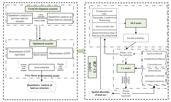
Figure 1.
Research framework.
2.2. Gray Linear Planning Model for the Determination of Land Use Structure
The gray linear planning model is a dynamic linear planning approach; its technological coefficient and constraint value are variable gray numbers. It can not only identify the optimal structure under given conditions but can also predict development changes in the optimal structure. Therefore, the gray linear planning model is widely used. The gray linear planning model is expressed as:
where f(x) is the objective function and s.t. is a constraint. xj is a decision variable and cj is the benefit coefficient of different land use types per unit area. aij is the coefficient of variable j in constraint i.bj is the constraint value.
2.2.1. Objective Function
In this study, eight land use types were investigated, namely, farmland, forest, grassland, waters, urban settlement, rural settlement, other built-up land, and unused land. and they were set as eight variables: x1, x2, x3, x4, x5, x6, x7, and x8. The optimized scenario aims to achieve maximum ESV while protecting the social reality of economic development and grain demands. Therefore, the ESV of the region should be calculated firstly. ESV in this study was calculated according to the following formula:
where ESV refers to the ecosystem service value (100 million RMB). Ak refers to the area of land use type k (hm2). VCk is the ecological service coefficient of land use type k (RMB/(hm2·a)). n is the number of land use types.
Based on Costanza et al. [17] and Xie et al.’s parameters (2015) [18], we extracted the equivalent weight factor of ecosystem services per hectare of terrestrial ecosystems in China (Table 1) and applied it to Puge County. The average natural food production of farmland per hectare per year was used to define a standard unit (1) of ecosystem service value. Generally, the natural food production is proposed to be 1/7 of the actual food production. According to the data in statistical yearbook of Puge County and the China Yearbook of Agricultural Price Survey, the economic benefit of grains in Puge County was 7768 RMB/hm2 from 2010 to 2014, manifested by a grain output per unit area of about 3884 kg/hm2 and an average selling price of 2 RMB/kg. Hence, the ecosystem service value of one equivalent weight factor for the Puge County is, therefore, 1109.7 Yuan.

Table 1.
Equivalent weight factor of ecosystem service per hectare of terrestrial ecosystems in China.
The ecosystem service value of per unit area of each land cover category in Puge County was then assigned based on the corresponding equivalent ecosystems (Table 2).
Table 2.
Ecosystem service value (ESV) per unit area of Puge County (yuan/hm2).
Based on the calculated ESV coefficient of different land use types, the objective function under the optimized scenario can be calculated as follows: F(x) = max Z = 3961.6 × x1 + 19774.9 × x2 + 15613.5 × x3 + 126128.5 × x4 − 9607.9 × x5 − 9607.9 × x6 − 9607.9 × x7 + 210.8 × x8.
2.2.2. Constraints
Different land use types focus on different constraints. According to regional natural, social, ecological conditions and planning requirements, the constraints and scope of the area of different land use types in the optimized scenario are set in Table 3.
Table 3.
Constraints and scope of the area of land use types under the optimized scenario.
2.3. MLP-CA Model for the Spatial Allocation of Land Use
An MLP-CA model was developed independently by combining multi-layer perception (MLP) [19] and cellular automaton (CA) [20]. Based on the MLP-CA model, corresponding transformation rules and principles were superposed to achieve the spatial allocation of the land use structure.
The MLP-CA model contains two modules, a training module and a simulation module. The training module is primarily realized by MLP and the simulation module is realized under the assistance of CA. The main process involves the automatic acquisition of internal transformation rules using training data in the training module; then, the external transformation rule is superposed. Later, these transformation rules are input to the simulation module to complete land use allocation [21]. The detailed process is described below.
The training module is primarily responsible for two tasks: the first is to determine the structure of MLP and the second is to acquire the internal transformation rule through training data and target data and then output the probability of occurrence of different land use types. Meanwhile, a certain amount of training data and verification data are selected in the training process to verify the accuracy of the constructed MLP. Only the internal transformation rules produced from training under satisfactory training accuracy and verification accuracy are applicable to subsequent studies; otherwise, the data must be selected again, and the above training process must be repeated.
After the probability of occurrence of different land use types is determined, the external transformation rules are set in accordance with actual needs. The external rules include the quantity of land use types, the absolute restricted area, ecological sensitivity, neighborhood influence, land transfer cost, and the self-adaptive inertia coefficient.
(a) Quantity of land use types
Quantity of land use types reflects the development direction of land use. The sum of the areas of different land use types at different times is constant and is equal to the total land area. It can be expressed as a function:
where total area is the total land use area. x1 to xn are areas of different land use types. n is the land use type. The quantity constraint is used as the overall control during land use allocation. In other words, the quantity of land use transformation at a certain time, which is an essential constraint, is determined. Quantity of land use can be gained from the land use distribution map during a certain period; future quantity of land use is based on the simulation results.
(b) Absolute restricted area
The absolute restricted area is the area where land use transformation is restricted. The allocation of this region cannot be changed. These areas generally include cliffs, natural reserves, extensive water surfaces, and basic farmlands protecting regional food safety. The absolute restricted areas data are binary data with values of 0 or 1. A value of 1 reflects an absolute restricted space, indicating that land use transfer is prohibited in this region. A value of 0 indicates non-absolute restricted space, meaning that land use transfer is allowed in this region.
(c) Ecological sensitivity
To achieve maximum ecosystem service functions in national key ecological function zones, ecosystem structures and functions must be kept in the most stable state and must protect the maximum value of the ecosystem service. Hence, ecological sensitivity is added as another constraint in this study. Ecological sensitivity restricts transfer among different land use types to some extent. The factor weighting method is usually applied for ecological sensitivity evaluation. Ecological sensitivity can be expressed as:
where f(xk) is the comprehensive value of ecological sensitivity. x1 to xn are influencing factors. In this study, slope, altitude, land use type, river, geological disaster liability, and soil erosion were chosen as the main influencing factors for the evaluation of ecological sensitivity. α1 to αn are the weights of different influencing factors; they are determined by the analytic hierarchy process (AHP).
Based on the ecological sensitivity evaluation results, regions ranking in the top 20% (regions with high ecological sensitivity) are viewed as regions where land transfer is prohibited; these are set as 0. The remaining 80% of regions (regions with small ecological sensitivity) are viewed as regions allowing land transfer; these are set as 1.
(d) Neighborhood influence
Cellular expansion is influenced by cells in a neighborhood except for itself. In the MLP-CA model, the neighborhood analysis window was set as 7×7 to define the influence of neighborhood cells on central cells. The neighborhood function is defined as:
where is the extent of grid cells affected by neighboring land use type j at time t, and represents the total number of grid cells occupied by land use type j at the last iteration time t–1 within the 7 × 7 window. wk is the variable weight among the different land use types, because there are different neighborhood effects for different land use types.
(e) Land transfer cost
Land transfer cost is mainly used to reflect difficulties in transformation among different land use types. When it is difficult to transform a particular land use type into another type, the land transfer cost is relatively high. When it is easy to transform a land use type into another type, the land transfer cost is relatively low. Land transfer cost is binary and is expressed as 0 or 1. Regions with low land transfer cost are 0, while regions with high land transfer cost are 1.
(f) Self-adaptive inertia coefficient
A self-adaptive inertia coefficient for each land use type is defined to auto-adjust the inheritance of the current land uses on each grid cell according to differences between the macro demand and the allocated land use amount. The inertia coefficient is defined as:
where, denotes the inertia coefficient for land use type j at iteration time t. and denote the difference between the macro demand and the allocated amount of land use type j at iteration time t−1 and t–2, respectively.
Next, the possibility of occurrence of land use types, which is generated automatically in the training model, as well as neighborhood influence, land transfer cost, and the inertia coefficient are combined to construct a comprehensive transfer probability index:
where is the comprehensive probability for cell i to transfer from the original type to type j at time t. is the probability of occurrence of land use type j on cell i. is the neighborhood expansion factor of land use type j on cell i at time t. is the inertia coefficient of land use type j at time t. is the transfer cost of the original land use type c to the target type j.
After obtaining the comprehensive transformation probability of the cells, the spatial allocation of land use is accomplished in the simulation module by superimposing a restriction area, ecological sensitivity constraints, and the quantitative structure of land use. However, there may be conflicts among the different rules in the allocation process. For example, a cell might be transferred from forest to farmland in view of the comprehensive transformation probability, but the cell might belong to a restricted area with land use transfer prohibited. Hence, several principles are defined in case of conflicts among transformation rules. (1) The preferential principle of the ecology: different land use types are distributed according to the following order: forest > grassland > waters > farmland > urban settlement > other built-up land > rural settlement > unused land; (2) The principle of maximum comprehensive transformation probability: taking forest, for example, different grids are ordered according to the comprehensive transformation probability [22]. The grids with the highest transformation probability (forests) are recognized. The grids are ranked from high to low transformation probability until the desired total amount of forest is met.
2.4. Selection and Implications of Landscape Indices
Landscape indices reflect the landscape structural composition, spatial allocation, etc. The effects of land use optimization under different scenarios were evaluated with type level and landscape level indices. In this study, the percentage of landscape (PLAND), landscape shape index (LSI), intersperse-juxtaposition index (IJI), and aggregation index (AI) were chosen as the type level indices. The contagion index (CONTAG), connection index (CONNECT), cohesion index (COHESION), AI, and Shannon diversity index (SHDI) were chosen as the landscape level indices. Formulas and the implications of the different indices are discussed in several references [23,24].
3. Study Area and Data
3.1. Study Area
Puge County is a mountainous county in southwest China, in the southeast of Sichuan Province (27°13’-27°30’N, 102°26’-102°46’E), covering an area of 1918 km2 (Figure 2). The Zemu River and Xiluo River are the main water resources in Puge County. There is diversified vegetation in Puge Country, with a vegetation coverage of 41.92%. In 2017, Puge County was enlisted as a national key ecological function zone in China; its purpose was the conservation of water and soil. To realize its ecological function orientation, Puge County is required to reduce or prohibit large-scale construction activities and strengthen ecological protection. However, the gross domestic product (GDP) in Puge County was only 2465.28 million RMB in 2017, and the per capita net income of peasant households was only 8734 RMB, which is lower than the national average levels during the same period. Therefore, there is an important internal demand for economic development and eradication of poverty in Puge County. Thus, Puge County must identify ways to achieve a protection-development balance by obtaining maximum ecological benefits while protecting social and economic development.
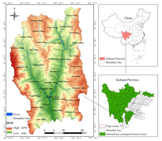
Figure 2.
Location map of Puge County.
3.2. Data Resources and Processing
Land use data of Puge County in 2010 and 2017 are from its Bureau of Land and Resources, which adopts the land use classification system of the Chinese Academy of Sciences (CAS) and is divided into eight categories (as mentioned above). Statistical survey data on land use changes (2010–2016), overall land use planning (2006–2020), distribution maps of geological disasters, areas, and location of towns, as well as data on rivers and roads, were all collected from local national land resources departments. According to road and river data, buffer zones are generated to obtain the distance to roads and rivers, which are important influencing factors of land use change, and it is for subsequent research. Urban planning information for Puge County (2013–2030) and the ecological safety control region were provided by the urban planning department. Statistical data came from the Statistical Bureau of Puge County. Among the statistical data, the spatial distribution map of population density is obtained by the spatial interpolation of its statistical data in each town. Meanwhile, the spatial distribution map of GDP is obtained by the spatial interpolation of its statistical data and the correction with GDP spatial data from China’s GDP distribution kilometer grid data set. Digital elevation model (DEM) data came from GS Cloud (http://www.gscloud.cn/) with a size of 30*30m. Based on DEM data, regional slope data is generated, and the topographical relief data is obtained by selecting 11*11 cells as the best statistical unit. Meteorological data came from the National Meteorological Center (http://data.cma.cn/). Meteorological factors, including annual average temperature and total annual precipitation, are obtained by the spatial interpolation of meteorological observation data and format conversion. Soil erosion data were collected from the Geographical Information Monitoring Cloud Platform (http://www.dsac.cn/); the data were unified to 30*30 m through resampling.
4. Results
4.1. Land Use Changes and Reasonability Analysis
In Puge County, forest and grassland were the dominant land use types, accounting for 78% of the total area. Farmland was the second largest land use type, accounting for 17% of the total area. Other land use types generally occupied small areas. From 2010 to 2017, areas of farmland, forest, and grassland decreased by 25.74, 53.43, and 133.12 hm2, respectively, while waters, urban settlement, rural settlement, and other built-up land areas increased by 4.37, 44.54, 121.47, and 42.38 hm2, respectively. The area of unused land changed only slightly, decreasing by 0.51 hm2. Generally speaking, the rural settlement area expanded the most. Due to the hollowing out of the population in rural areas, intensive land use was impacted, to some extent. Moreover, forest and grasslands were expropriated the most, which violates the regional policy of returning grain plots to forestry (grassland); this trend has an impact on regional ecological safety.
A total area of 523.15 hm2 underwent changes in land use types (Figure 3). Specifically, 204.88 hm2 of farmland was transferred to other land use types (mainly rural settlement). Forest areas (88.4 hm2) were reclaimed by other land used types, mainly by farmland and rural settlements. The grassland area decreased by 169.8 hm2; this was mainly due to transference to farmlands. The transfer of other land use types was insignificant. Generally, large areas of forest and grassland were transferred to farmland between 2010 and 2017, reflecting the prominent deforestation and reclamation of wastelands in this region. Meanwhile, farmland, forest, and grassland were overtaken by built-up land, which may disrupt ecological functional stability if no appropriate controlling measures are taken. Hence, it is necessary to optimize land use types by targeting the maximum value of ESs.
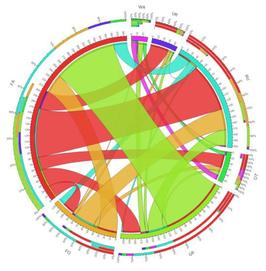
Figure 3.
Land use transfer from 2010 to 2017. Notes: FA refers to farmland. FO is forest. GR is grassland. WA is waters. UR is urban settlement. RU is rural settlement. OT is other built-up land. UN is unused land.
4.2. Multi-Scenario Analysis of Land UseStructure
Based on the areas of different land use types in Puge County from 2010 to 2016, areas of different land use types in 2030 under the trend development scenario were predicted through linear regression and the GM (1,1) model. Prediction functions, judgment coefficients and area of different land use types are shown in Table 4.
Table 4.
Prediction functions, judgment coefficients, and area of different land use types.
The gray linear planning model was solved in LINGO software according to the area scope of different land use types and objective function, thus obtaining the quantitative structure of land use types in Puge County in 2030 under the optimized scenario (Table 5). Table 4 shows that, under the trend development scenario, farmland and settlements will be further expanded compared with data in the base year (2017), while areas of forest and grassland will be decreased. However, the opposite phenomena are observed under the optimized scenario. The quantitative structure of land use types under the trend development scenario differs greatly from the future development planning of Puge County. Moreover, the ESV under the optimized scenario is 3.32 billion RMB, which is higher than that in the base year (3.22 billion RMB) and higher than that under the trend development scenario (3.20 billion RMB). Hence, the optimized land use structure can increase the ESV of land resources without sacrificing economic benefits, grain demands, and relevant planning.
Table 5.
Area of land use types under different scenarios (hm2, %, 108yuan).
4.3. Spatial Allocation of Land Uses
Based on the training module of the MLP-CA model, the land use distribution map and the influencing factors (e.g., altitude, slope, topographical relief, distance to roads, distance to rivers, annual average temperature, total annual precipitation, population density, and GDP) in Puge County in 2010 were used as the input layer to train the multi-layer perception. Four hidden layers were discovered in the multi-layer perception after the completion of training. The number of nodes in each layer was 64, 128, 512, and 8, respectively. The excitation function of the first three layers was relu and the fourth was softmax. The training network was verified by random sampling. A total of 185,586 training samples and 79,538 verification samples were collected. In Figure 4, convergence of data error in the initial stage of training can be observed. However, data error decreases gradually with increasing iterations and the curve tends to be straight accordingly. As approaching to 500 iterations, the error curve is approximately parallel, which indicates that there is a small amount of error; this signals the termination of data training. The training accuracy and verification accuracy reached 82.38% and 80.72%, which are satisfactory. Moreover, the receiver operating characteristic curve (ROC, Figure 5) of the probability of occurrence of each land use type is drawn. It is found that the area under ROC (AUC) is greater than 0.7 except x8, and the simulation is accurate [25]. Therefore, the model is suitable for subsequent simulation.
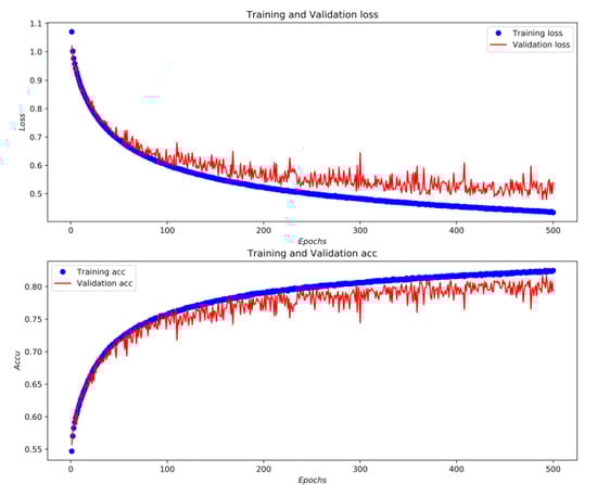
Figure 4.
Convergence curve.
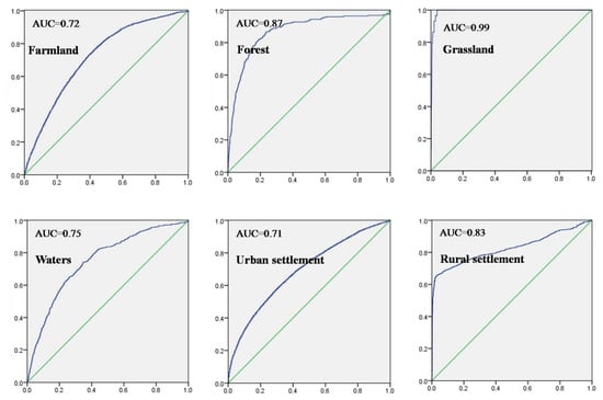
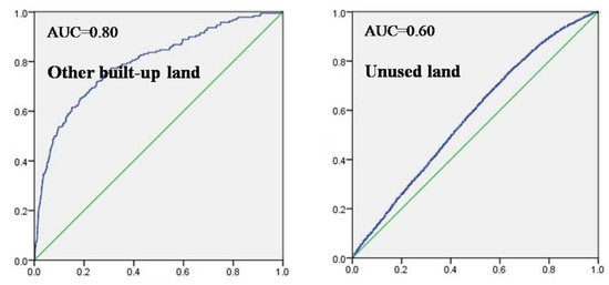
Figure 5.
Area under ROC (AUC) value of each land use type.
First, the neighborhood influence of central cells was calculated according to the neighborhood weight of different land use types. Second, the neighborhood influence of central cells was multiplied by the transfer cost, the self-adaptive inertia coefficient of different land use types, and the possible probability of the occurrence of different land use types to obtain the comprehensive transformation probability. Third, the ecological sensitivity map (Figure 6) and restricted area (Figure 7) in Puge County in 2010, as well as the quantitative structure of land use in 2017, were superposed. Finally, the spatial allocation of land uses in Puge County in 2017 was completed in the simulation module according to the relevant principles (Figure 8 and Figure 9).
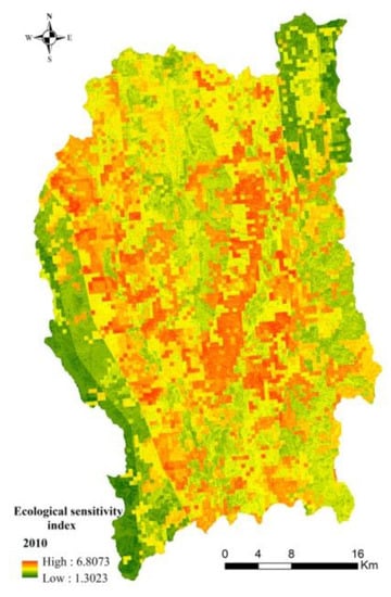
Figure 6.
Ecological sensitivity in 2010.
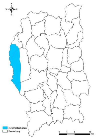
Figure 7.
Restricted area of Puge County.
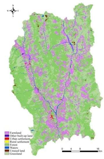
Figure 8.
Actual distribution map of land use in Puge County in 2017.
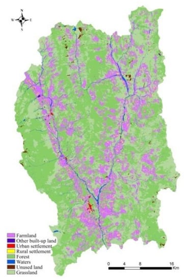
Figure 9.
Simulated distribution map of land use in Puge County in 2017.
Then, the simulation map and actual distribution map of land use types in Puge County in 2017 were used as the basis to calculate the grid number and Moran’I index among different land use types. The accuracy of the number of grids in different land use types was higher than 99% and the Moran’I index between simulation and actual distribution map was close. This indicates that the parameters were set appropriately and that the simulation effect was good in this study; thus, this methodology is applicable to subsequent studies.
The distribution map of land use and corresponding influencing factors in 2017 were used as the input data and the probability of occurrence of different land use types was obtained according to the above trained network. Then, the neighborhood influence of central cells was calculated according to the neighborhood weight of different land use types. The neighborhood influence of central cells was multiplied by the transfer cost, the self-adaptive inertia coefficient of different land use types, and the possible probability of occurrence of different land use types to obtain the comprehensive transformation probability. Then, the ecological sensitivity distribution map and restricted area map of Puge County in 2017, as well as the land use structure in 2030, were superposed. Finally, the spatial allocation of land use in Puge County in 2030 was completed in the simulation module (Figure 10 and Figure 11). It can be seen that the distributions of farmlands, forests, grasslands, and rural settlement were different under different scenarios. Forests and grasslands expanded toward the external sides of rivers and at high altitudes in a “Y-shaped” pattern under the optimized scenario. Farmlands expanded towards basin areas between rivers in a “Y-shaped” pattern under the trend development scenario. Rural settlements spread from the urban center under the trend development scenario. Abundant farmlands, forests, and grasslands were overtaken by rural settlements.
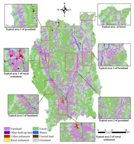
Figure 10.
Spatial distribution of land use under the trenddevelopment scenario in 2030.
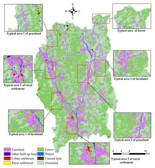
Figure 11.
Spatial distribution of land use under the optimized scenario in 2030.
5. Discussion
5.1. Method Research
The land use optimization framework proposed in this study realizes the combination of quantitative structure simulation and spatial allocation, and has an important reference value for future land use planning and layout. At the same time, the MLP-CA model is developed independently by combining a multi-layer neural network with cellular automata, which avoids the defects caused by a single method and improves the simulation accuracy. However, like other methods, the MLP-CA model also has some shortcomings, which can not reflect the physical mechanism between internal elements. Moreover, the transformation rules in this study are mainly set for ecologically sensitive (fragile) areas, and its universality is limited.
5.2. Multi-Scenario Optimization Effect in Puge County
5.2.1. Evaluation of Landscape Pattern Effect under Different Scenarios
With respect to type level (Table 6), forest and grassland possess absolute advantages in terms of PLAND. The PLAND of forest and grassland was the lowest under the trend development scenario and was highest under the optimized scenario. The LSI of forest and grassland was high under the optimized scenario; this is primarily related to the large area of forests and grasslands. Moreover, the areas of other built-up land were highly fragmented, exhibiting a more complicated spatial structure. Therefore, the LSI of other built-up land was higher compared with that of rural settlements. The IJI of settlements was high under the optimized scenario, indicating that settlements were surrounded by different land use types and there was good integration and strong extension of different land use types under the optimized scenario. The AI of forest and urban settlements under the optimized scenario was higher compared with that under the other two scenarios. Forest and urban settlement had strong spatial aggregation under the optimized scenario, with expansion predicted toward sheet and bulk development.
Table 6.
Landscape index at type level in Puge County from 2017 to 2030 (%).
With respect to the landscape indices (Table 7), the CONTAG was the highest under the optimized scenario and the smallest under the trend development scenario, indicating that the landscape has good ductility under the optimized scenario. The CONNECT index was the same under the different scenarios (0.05%). The COHESION index was the highest under the optimized scenario and its value under the trend development scenario was the same as that in 2017. To sum up, landscape intensity and stability are stronger under the optimized scenario. The AI reached a peak under the optimization situation and was lowest in the trend development scenario, indicating the strongest degree of aggregation of landscapes under the optimized scenario. The SHDI was the highest under the trend development scenario, followed by the optimized scenario, and then 2017. While the SHDI under the trend development scenario was the highest, which is advantageous for improving regional microclimate, this finding also suggests that the degree of plaque fragmentation under the trend development scenario is higher, which violates the concept of intensive utilization of regional space. Therefore, the plaque area must be expanded appropriately while protecting biological and landscape diversity in order to increase the aggregation and contagion of different plaques. These requirements are met under the optimized scenario.
Table 7.
Landscape index at landscape level in Puge County from 2017 to 2030 (%).
With respect to the type and landscape scale, land use type under the optimized scenario was more beneficial to aggregation and spread of different landscape plaques while protecting biological and landscape diversity. The overall ecological effect of the region was improved by connecting and spreading of different plaques.
5.2.2. Land Use Distribution under Different Topographical Conditions
Land use type, structure, and characteristics are obviously different under different topographic conditions. In this study, three typical topographical factors (i.e., altitude, slope and relief amplitude) were chosen to discuss the reasonability of the land use layout under different scenarios from a microscopic perspective. Based on the characteristics of mountainous regions and the practical requirements of these regions, altitude, slope, and relief amplitude were divided into five levels (altitude: <1500, 1500–2000, 2000–2500, 2500–3000, and >3000 m; slope: 0°–3°, 3°–8°, 8°–15°, 15°–25°, and >25°; relief amplitude: <30, 30–50, 50–100, 100–150, and >150 m).
Figure 12a shows that the area of farmland at altitudes above 2500–3000 m under the optimized scenario was the smallest. The cultivation condition of farmland in high altitude is poor, the marginal income is low, and unreasonable development is proneto ecological security problems [26]. So, the farmland area in high altitude should be appropriately reduced, and the optimized scenario is just in line with this demand. Moreover, the area of rural settlement at altitudes above3000mwas smaller under the optimized scenario (Figure 12b), which is not only safer, but also provides more available land resources for this region. The area of unused land at low altitude under the optimized scenario was the smallest, which reflects the highest utilization intensity; this conforms to the regional planning of intensive and economical land use.
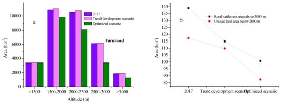
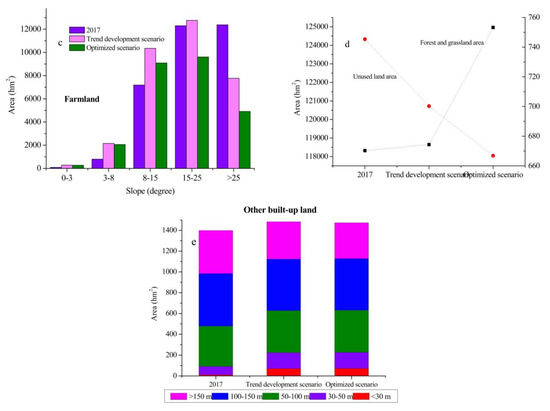
Figure 12.
Comparison of area of land use under different scenarios (hm2). (a) The area of farmland on different altitudes; (b) the areas of rural settlement above 3000 m and unused land below 2000 m; (c) the areas of farmland on different slopes; (d) the area of forest, grassland and unused land on slopes above 15°; (e) the area of other built-up land on different relief amplitude.
On different slopes, the area of farmland was decreased to the maximum extent under the optimized scenario (Figure 12c). The farmland quality on the steep slope of Puge County is not high, when it is developed unreasonably, it is likely to have soil erosion and other problems, which will affect regional ecological security. For this reason, the policy of returning farmland to forest (grassland) has been adopted to promote the transformation of farmland on steep slope to forest or grassland. Obviously, the implementation intensity under the optimized scenario is greater. Moreover, forest and grassland on slopes above 15° under the optimization scenario were generally increased, while unused land was generally decreased (Figure 12d), which is consistent with the result of Figure 12c, and ensures the stability of regional ecological security.
The geological environment in areas with large relief amplitude is generally active, and the development of industrial and mining production activities in these areas is faced with greater safety risks [27]. It can be seen from Figure 12e that the area of other built-up landon relief amplitude above 150 m under the optimization scenario is the smallest, which means the safety under optimized scenario is relatively high.
In summary, compared with the trend development scenario, the land use distribution at different topographical conditions under the optimized scenario is more reasonable.
6. Conclusions
Construction demands continue to increase as a result of economic development and urbanization; this intensifies ecological environmental damage. In return, the impact of ecosystem damage is fed back to human beings, thus hindering sustainable development of these regions. Therefore, land use optimization is critical. As a method to evaluate ecological service functions of land resources, ESV is an important index that measures whether regional land use layout is reasonable and whether ecological safety is protected. Land use optimization based on ESV is of great significance for solving conflicts between social and economic development and environmental protection, and for promoting sustainable development of regions.
A framework for land use decisions based on quantitative analysis and spatial allocation of land use was proposed. In this, multiple scenarios were set in the quantitative analysis of land use structure. The trend development scenario was established by solving linear regression and the GM (1,1) model based on the previous land use structure. The optimized scenario was built by solving the gray linear planning model with consideration for planning, policy, and practical constraints in areas of different land use types. The aim of this was to maximize the ESV. Setting multiple scenarios is conducive to contrast analysis and achieving the orientation of different ecological function zones. An MLP-CA model was developed for spatial allocation of land use by combining multi-layer perception and cellular automaton. This MLP-CA model comprised multiple hidden layers in the training module, which can significantly increase the accuracy of training results. Moreover, this model gives full consideration to the actual ecological demands and characteristics of this region and sets several external rules, such as restricted areas and ecological sensitivity evaluation based on the comprehensive transformation probability; this was in order to protect the stability of the ecosystem during spatial allocation. Furthermore, the rules of ecological priority and probability maximization were adopted in the allocation module to prevent conflicts of different rules; this assured unique and accurate spatial allocation of land uses. As a systematic technological framework for land use decisions, the proposed framework provides a new perspective for coordination between ESs and land use management.
According to our empirical study of the proposed framework based on Puge County, the quantitative structure of land use under the trend development scenario in 2030 was significantly different from future development planning in Puge County. In terms of spatial layout, land use types under the trend development scenario were highly fragmented with weak spatial correlations; this is at odds with intensive land use. While land use under the optimized scenario not only protected the ecological safety of goods in the region, met the relevant local and national policy requirements and regulations, but also strengthened spatial relations of different land use types allowing the maximum output of ecological benefits. Land use layout under the optimized scenario provides an alternative program for future land planning, relieves conflicts among different land use types, and improves ecosystem service ability in Puge County.
Author Contributions
Li Peng, Tiantian Chen and QiangWang conceived and designed the research; Tiantian Chen and Qiang Wang conducted the literature review; Tiantian Chen and Li Peng analyzed the data; Li Peng, Tiantian Chen, Qiang Wang and Wei Deng wrote the paper. All authors have read and agreed to the published version of the manuscript.
Funding
This study was supported by the Science and Technology Service Initiative (No. KFJ-STS-QYZD-060), the National Natural Science Foundation of China (No. 41771194) and Chongqing Normal University funding project (19XLB015).
Conflicts of Interest
The authors declare no conflict of interest.
References
- Verónica, C.; Diego, P.V.; Amoroso, M.M.; Bennett, E.M. Land use intensity indirectly affects ecosystem services mainly through plant functional identity in a temperate forest. Funct. Ecol. 2018, 2, 1365–2435. [Google Scholar]
- Pattanayak, S.K. Valuing watershed services: Concepts and empirics from southeast Asia. Agric. Ecosyst. Environ. 2004, 104, 171–184. [Google Scholar] [CrossRef]
- Loomis, J.; Kent, P.; Strange, L.; Fausch, K.; Covich, A. Measuring the total economic value of restoring ecosystem services in an impaired river basin: Results from a contingent valuation survey. Ecol. Econ. 2000, 33, 103–117. [Google Scholar] [CrossRef]
- Peng, L.; Deng, W.; Zhang, H.; Sun, J.; Xiong, J. Focus on economy or ecology? A three-dimensional trade-off based on ecological carrying capacity in southwest China. Nat. Resour. Model. 2018, 32, e12201. [Google Scholar]
- Li, Y.R.; Cao, Z.; Long, H.; Liu, Y.; Li, W. Dynamic analysis of ecological environment combined with land cover and NDVI changes and implications for sustainable urban–rural development: The case of Mu Us Sandy Land, China. J. Clean. Prod. 2017, 142, 697–715. [Google Scholar] [CrossRef]
- Ziter, C.; Turner, M.G. Current and historical land use influence soil-based ecosystem services in an urban landscape. Ecol. Appl. 2018, 28, 643–654. [Google Scholar] [CrossRef] [PubMed]
- Arowolo, A.O.; Deng, X.; Olatunji, O.A.; Obayelu, A.E. Assessing changes in the value of ecosystem services in response to land-use/land-cover dynamics in Nigeria. Sci. Total Environ. 2018, 636, 597–609. [Google Scholar] [CrossRef]
- Cerretelli, S.; Poggio, L.; Gimona, A.; Yakob, G.; Boke, S.; Habte, M.; Coull, M.; Peressotti, A.; Black, H. Spatial assessment of land degradation through key ecosystem services: The role of globally available data. Sci. Total Environ. 2018, 628, 539–555. [Google Scholar] [CrossRef]
- Bryan, B.A.; Crossman, N.D. Impact of multiple interacting financial incentives on land use change and the supply of ecosystem services. Ecosyst. Serv. 2013, 4, 60–72. [Google Scholar] [CrossRef]
- Shoyama, K.; Yamagata, Y. Predicting land-use change for biodiversity conservation and climate-change mitigation and its effect on ecosystem services in a watershed in Japan. Ecosyst. Serv. 2014, 8, 25–34. [Google Scholar] [CrossRef]
- Daniels, A.E. Patterns and Processes of Land Cover Change: Understanding Tradeoffs Among Ecosystem Services; University of Florida, Proquest Dissertations Publishing: Gainesville, FL, USA, 2009. [Google Scholar]
- Cheng, F.; Liu, S.; Hou, X.; Zhang, Y.; Dong, S. Response of bioenergy landscape patterns and the provision of biodiversity ecosystem services associated with land-use changes in Jinghong County, Southwest China. Landsc. Ecol. 2018, 33, 783–798. [Google Scholar] [CrossRef]
- He, L.; Jia, Q.; Li, C.; Zhang, L.; Xu, H. Land use type simulation based on ecosystem service value and ecological security pattern. Trans. Chin. Soc. Agric. Eng. 2016, 32, 275–284. (In Chinese) [Google Scholar]
- Wu, X.; Wang, S.; Fu, B.; Liu, Y.; Zhu, Y. Land use optimization based on ecosystem service assessment: A case study in the Yanhe watershed. Land Use Policy 2018, 72, 303–312. [Google Scholar] [CrossRef]
- Fan, J.; Sun, W.; Zhou, K.; Chen, D. Major function oriented zone: New method of spatial regulation for reshaping regional development pattern in China. Chin. Geogr. Sci. 2012, 22, 196–209. [Google Scholar] [CrossRef]
- Li, X.; Yu, T.; Yuan, Z. Model GM (1,1,β) and its applicable region. Grey. Syst. 2013, 3, 266–275. [Google Scholar] [CrossRef]
- Costanza, R.; D’Arge, R.; De Groot, R.; Farber, S.; Grasso, M.; Hannon, B.; Limburg, K.; Naeem, S.; O’Neill, R.V.; Paruelo, J.; et al. The value of the world’s ecosystem services and natural capital. Nature 1997, 387, 253–260. [Google Scholar] [CrossRef]
- Xie, G.; Cao, S.; Yu, X.; Pei, X.; Bai, Y.; Li, W.; Wang, B.; Niu, X.; Liu, X.; Xu, Z.; et al. Ecosystem Service Evaluation. In Contemporary Ecology Research in China; Li, W., Ed.; Springer: Berlin/Heidelberg, Germany, 2015. [Google Scholar]
- Mizutani, E.; Dreyfus, S. An analysis on negative curvature induced by singularity in multi-layer neural-network learning. Adv. Neural. Inf. Process. Syst. 2010, 23, 1669–1677. [Google Scholar]
- Bastien, C. Cellular Automata Modeling of Physical Systems. Comput. Complex. 2012, 3, 407–433. [Google Scholar]
- Li, X.; He, J.; Liu, X. Ant intelligence for solving optimal path-covering problems with multi-objectives. Int. J. Geo. Inf. Sci. 2009, 23, 839–857. [Google Scholar] [CrossRef]
- He, C.Y.; Shi, P.J.; Li, J.G.; Pan, Y.Z.; Chen, J. Scenarios simulation land use change in the northern China by system dynamic model. Acta Geogr. Sin. 2004, 59, 599–607. (In Chinese) [Google Scholar]
- Rodríguez-Loinaz, G.; Alday, J.G.; Onaindia, M. Multiple ecosystem services landscape index: A tool for multifunctional landscapes conservation. J. Environ. Manag. 2015, 147, 152–163. [Google Scholar] [CrossRef] [PubMed]
- O’Neill, R.V.; Krummel, J.R.; Gardner, R.H.; Sugihara, G.; Jackson, B.; DeAngelis, D.L.; Milne, B.T.; Turner, M.G.; Zygmunt, B.; Christensen, S.W.; et al. Indices of landscape pattern. Landsc. Ecol. 1988, 1, 153–162. [Google Scholar] [CrossRef]
- Chen, Y.; Zhang, L.; He, L.; Men, M. Multi-scenario simulation of land use structure based on dual combined models. Acta Ecol. Sin. 2016, 36, 435–447. (In Chinese) [Google Scholar]
- Long, H.L. Land rehabilitation and regional land use transition. Prog. Geogr. 2003, 22, 133–140. (In Chinese) [Google Scholar]
- Cai, D.M.; Li, B.; Xu, W.S.; Zhang, P.C.; Hui, B. Relief degree of land surface in Hubei Province studied based on ASTERGDEM data and its correlations with population density and economic development. Bull. Soil Water Conser. 2017, 37, 231–234. (In Chinese) [Google Scholar]
© 2020 by the authors. Licensee MDPI, Basel, Switzerland. This article is an open access article distributed under the terms and conditions of the Creative Commons Attribution (CC BY) license (http://creativecommons.org/licenses/by/4.0/).