Article

Spatial Assessment of the Effects of Land Cover Change on Soil Erosion in Hungary from 1990 to 2018

Faculty of Agricultural and Environmental Sciences, Szent István University, 2100 Gödöllő, Hungary
*
Author to whom correspondence should be addressed.
ISPRS Int. J. Geo-Inf. 2020, 9(11), 667; https://doi.org/10.3390/ijgi9110667
Submission received: 2 October 2020 / Revised: 29 October 2020 / Accepted: 30 October 2020 / Published: 6 November 2020

Abstract

:
As soil erosion is still a global threat to soil resources, the estimation of soil loss, particularly at a spatiotemporal setting, is still an existing challenge. The primary aim of our study is the assessment of changes in soil erosion potential in Hungary from 1990 to 2018, induced by the changes in land use and land cover based on CORINE Land Cover data. The modeling scheme included the application and cross-valuation of two internationally applied methods, the Universal Soil Loss Equation (USLE) and the Pan-European Soil Erosion Risk Assessment (PESERA) models. Results indicate that the changes in land cover resulted in a general reduction in predicted erosion rates, by up to 0.28 t/ha/year on average. Analysis has also revealed that the combined application of the two models has reduced the occurrence of extreme predictions, thus, increasing the robustness of the method. Random Forest regression analysis has revealed that the differences between the two models are mainly driven by their sensitivity to slope and land cover, followed by soil parameters. The resulting spatial predictions can be readily applied for qualitative spatial analysis. However, the question of extreme predictions still indicates that quantitative use of the output results should only be carried out with sufficient care.

1. Introduction

Soil erosion by water continues to be a significant degradation process for soil resources around the world. Due to the expected increased occurrence of extreme precipitation events, soil erosion remains a key threat to soil resources [1,2,3]. Therefore, soil erosion by water is still in the focus of a number of global and regional policies [4].
In the past decades, a significant number or model-based soil erosion susceptibility mapping studies have been carried out worldwide [5]. Batista et al. [6] provided a review of recently applied soil erosion models, evaluation methods, and limitations.
A large portion of soil erosion modeling projects focused on the use of the empirical Universal Soil Loss Equation (USLE) [7] or its revised versions MUSLE [8,9] and RUSLE [10] in variable spatial and temporal scales. A growing number of applications are utilizing remotely sensed input data [11,12,13,14,15].
The Pan-European Soil Risk Assessment (PESERA) model was primarily developed for the regional scale estimation of rill and inter-rill erosion. As a process-based model, PESERA requires a significantly larger number of input data layers and a larger amount of processing power than the USLE model. Most recently Li et al. [5] have applied the PESERA model along with the RUSLE model. National level soil erosion maps in Hungary have first been founded on field-based expert knowledge [16]. In 2000, a 1:100,000 scale USLE based national erosion risk map has been compiled [17]. In 2016, Pásztor et al. [18] developed a new soil erosion risk map for Hungary, based on the USLE and PESERA models, focusing on the extreme wet year of 2010. This map was later adopted for the National Atlas of Hungary [19]. While the primary focus of soil erosion research in Hungary is erosion by water, there have also been recent studies focusing on susceptibility to wind erosion [18,20].
Since Hungary is still lacking a comprehensive national soil erosion monitoring network [21], proper validation and/or calibration of such maps has been a challenge. A semi-quantitative evaluation study has concluded that the map from the combined USLE–PESERA approach has been in line with in situ observations of farmers [22].
Land use and land cover (LULC) play a critical role in soil erosion processes. The changes in LULC can have significant effect on susceptibility to soil erosion [23,24,25], especially in case of agricultural land use [26,27,28], and, thus, can contribute to reductions in soil organic carbon (SOC) [29]. Therefore, understanding LULC dynamics and its effects on soil erosion can provide key information to decision makers [11,30,31,32,33].
Considering the effects of land use change on soil erosion, several studies have been focused on the assessment of LULC changes. One typical approach is the simulation of LULC change by different models. For example, Shrestha et al. [34] quantified the individual and integrated impacts of climate and land use change in stream flows in the Songkhram River. They used dynamic conversion of land use and its effects (Dyna-CLUE) as a land use change model to define land use change scenarios. Zhang et al. [35] used a combination of a Markov chain model and Dyna-CLUE model to simulate future land uses. Lamichhane and Shakya [36] also utilized a CLUE-S based approach to assess the impact of LULC and climate change on watershed hydrology. Another common methodology is based on using legacy information and/or satellite data for the assessment of LULC changes [37,38,39].
As the abovementioned studies show, both the USLE and the PESERA models are still being applied for evaluating the effects of changes in climate or in land use/land cover, even though there are clear differences in their predictions [40,41]. In their recent study, Ciampalini et al. [42] have performed a sensitivity analysis with the PESERA model, focusing on the effects of climatic parameters. However, there is still a lack of information regarding the effects of other input parameters, specifically the effects of land use/land cover.
In modeling situations, where sufficient validation data is not available, a potential method is the application of random forest variable importance measures in order to assess the sensitivity of models to particular input variables [43,44]. To our knowledge, this method has not yet been applied for the comparison of USLE and PESERA models.
The aim of the work presented here was to assess the extent of land cover changes in Hungary between 1990 and 2018, and to estimate the effects these changes had on soil erosion potential, while also providing a comparison of the two models and their sensitivity to input parameters through the application of random forest variable importance. Our basic assumptions include the established nature of the applied models (i.e., they provide valuable information regarding potential loss due to water erosion [18,22]), and reliability of the input datasets. Our base hypothesis is that LULC changes from 1990 to 2018 have influenced potential erosion rates. In order to make different years comparable, we have used the climate data of 2010 as a benchmark year.

2. Materials and Methods

The current study has adopted the methodology and the data utilized for the development of the Soil Erosion Map of Hungary [18]. While a national erosion monitoring network does not exist, this map (utilizing the 2006 CORINE Land Cover data) has been semi-quantitatively evaluated and is currently accepted at the national level [22,45]. In order to assess the effect of LULC change, all variables unaffected by such changes have been kept as stationary, focusing on the wettest observed year 2010 as climatic baseline.

2.1. Study Area

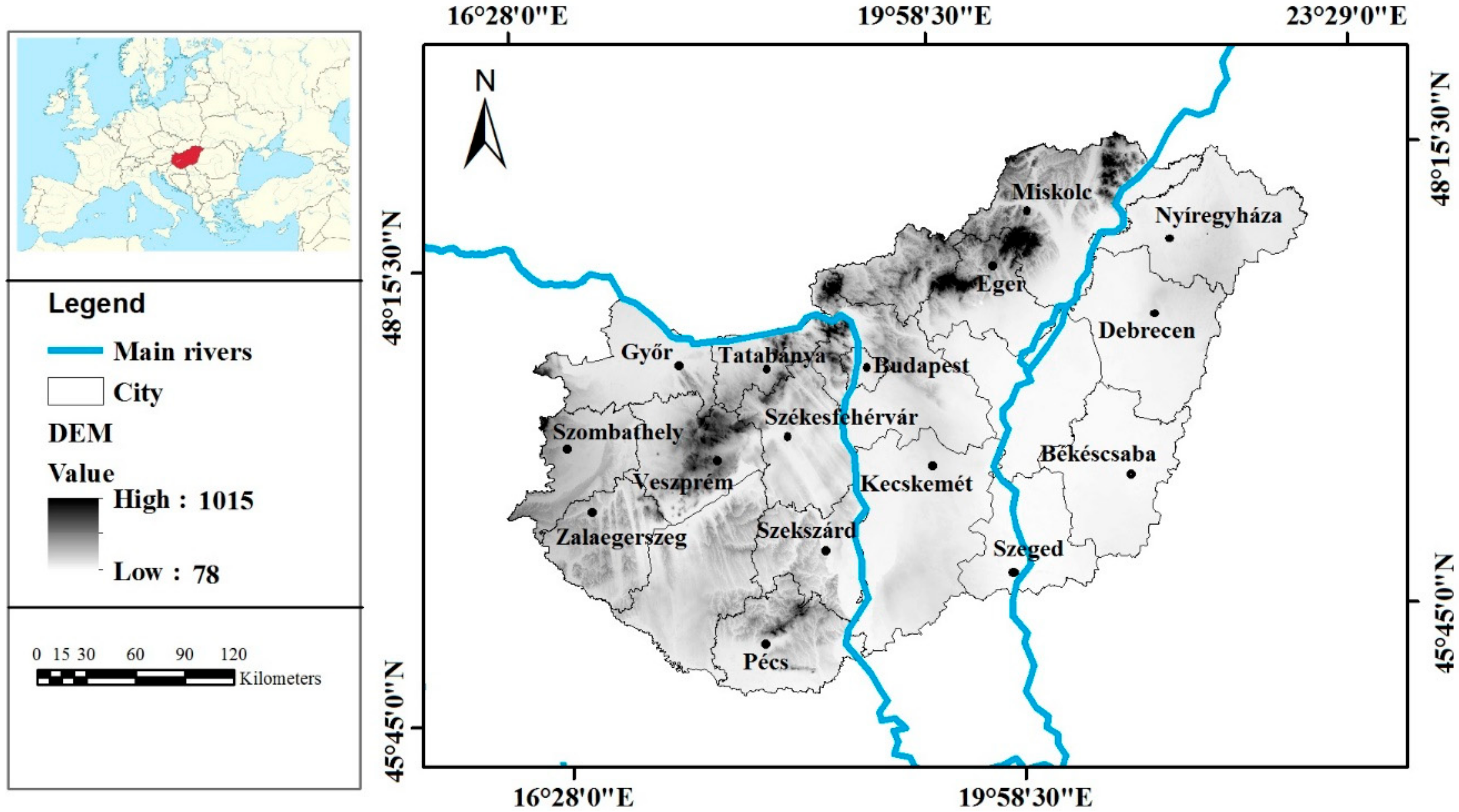
Hungary is situated in central Europe (45°48′ and 48°35′ N, 16°05′, and 22°58′ E), in the Carpathian Basin. Its highest peak is at 1014 m, while its lowest point is at 78 m. The whole area of the country is in the basin of the Danube River [19].
The relief of Hungary is mostly expressed as low elevation and low vertical dissection (Figure 1). The area is dominated by lowland regions (82.4% below 200 m), with only about 0.5% of terrain above 500 m. Medium-height mountains (200–500 m) cover 2.1% of the area, while hills and foothills 15.5%. [46]
Hungary is located in the northern temperate zone, but is influenced by three climatic zones (oceanic, continental and Mediterranean). Its climate is characterized by four seasons, with a great temporal variability. Typical climatic parameters for the whole of Hungary are presented in 
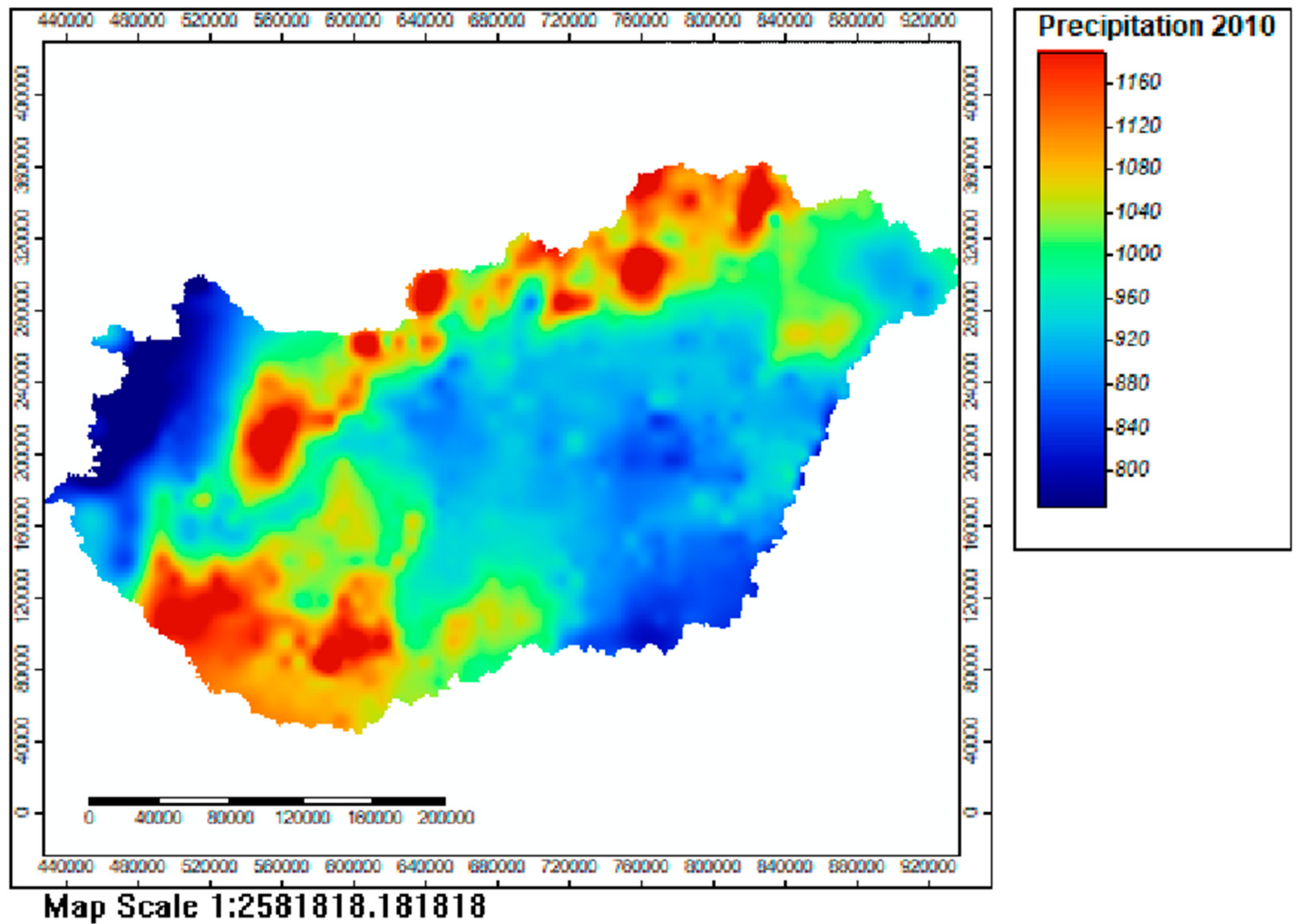
Table 1. Summer is the warmest season with the highest seasonal precipitation, while winter is typically the coldest and driest season. However, precipitation can be especially variable in the region both temporally and spatially. The wettest observed year was 2010, also having an average of 9 days with high (more than 20 mm) precipitation [47]. Recent studies have shown that while the spatial distribution of extreme (more than 40 or 60 mm) rainfall events has not changed significantly over the past decades, their intensity and frequency is showing an increasing tendency [48,49]. Figure 2 presents the spatial distribution of annual precipitation for the present study’s benchmark year 2010.
Amongst the different natural hazards in Hungary, mass movements (primarily landslides) are concentrating only in small areas, while soil erosion by wind can amount to as much as 80–110 million m3 annually, with 10% of the total area of the country being susceptible to wind erosion [45,50,51]. Soil erosion by water affects about 24.7% of the total area of Hungary [18,21].
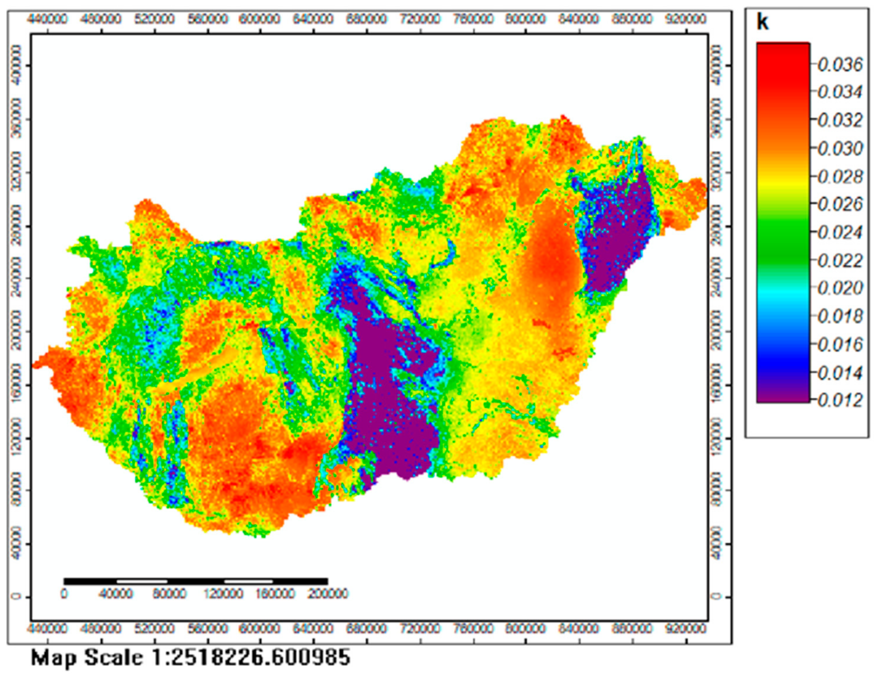
Hungary has a wide variety of soils. In hilly or mountainous areas, Luvisols and Cambisols are typical, while the Great Plain area has a range of Chernozems, Vertisols, Solonchaks and Solonetz soils. Alluvial plains often contain Luvisols, while certain areas with sand deposits have Arenosols dominating [52]. Figure 3 presents the spatial distribution of the USLE K factor in Hungary.
The vegetation of Hungary is mostly part of the Pannonian region, a forest steppe surrounded by the Turkey oak forest zone. The Carpathian Mountains are dominated by beech and spruce. Influenced by various biogeographic effects, the Pannonian region has a highly diverse vegetation with variable spatial distribution. Besides grasslands and dry oak forests, there is a high proportion of Sub-Mediterranean, continental and Balkan species, with Eurasian elements still dominant in most plant communities. [53]

2.2. Applied Models

2.2.1. The Universal Soil Loss Equation (USLE) Model

The empirical USLE model was the first widespread method to calculate soil loss. The model uses the following formula to calculate average annual soil loss A (t/ha-):
A = R × K × L × S × C × P
where R is the rainfall erosion index (MJ mm/ha/h/y), K is the soil erodibility factor (t × ha × h /ha/ MJ/mm), L is slope length factor and S is slope gradient factor, C is the cropping cover management factor, and P is the agricultural practice factor [7,21]. In case of the agricultural practice factor is not available, a default value of 1 can be used [21].

2.2.2. Pan-European Soil Risk Assessment (PESERA) Model

The process-based model partitions the precipitation into overland flow, evapotranspiration and soil moisture storage. It also includes a plant growth model to calculate biomass, leaf fall and vegetation cover. It generates daily rainfall using a monthly Gamma distribution. To compute total erosion, sediment yield Y is calculated by the expression:
Y =   ς k H r 2
where ς is the ratio of slope base to average gradient, k is the soil erodibility (kg liter-2 m day), H is the total slope length (m) multiplied by the average slope gradient and r is the local runoff in (mm) for each event. Detailed equations and model description are presented by Kirkby et al. [54].
The PESERA model requires a large number of input layers of which 96 relates to climate (rainfall, temperature, potential evapotranspiration), 25 to land use, crops, and planting dates (land cover type, dominant arable crops, planting dates, initial ground cover, initial surface storage, surface roughness reduction per month, root depth), 6 to soil parameters (crust storage, sensitivity to erosion, effective water storage capacity, soil water available to plants in top 300 mm, soil water available to plants, scale depth) and 1 to topography (standard deviation of elevation in a 1.5 km radius). Some climatic layers are optional and are only used in case of simulating climatic changes (not applicable for the current study). In case dominant crops are not available, a default assumption of maize can be applied to all arable land. Detailed description of model input parameters and application is presented in the PESERA Manual [55].

2.3. Data Sources and Processing

All source and input datasets (see Table 2) have been in a raster format, with their original grid size resampled and/or interpolated where necessary. The target grid size of the study was a 100 × 100 m (1 ha) grid.
Data processing and application of the USLE model (multiplication of its factors) was primarily carried out in ArcMap 10.1, while application of the PESERA model utilized ArcInfo Workstation 9.3 for pre- and post-processing. The PESERA model itself is a set of standalone executable and. aml files, including the model itself and data input/output [55]. Analysis, tables and graphs have been prepared with MS Excel and R software [56].

2.3.1. Land Use and Land Cover information

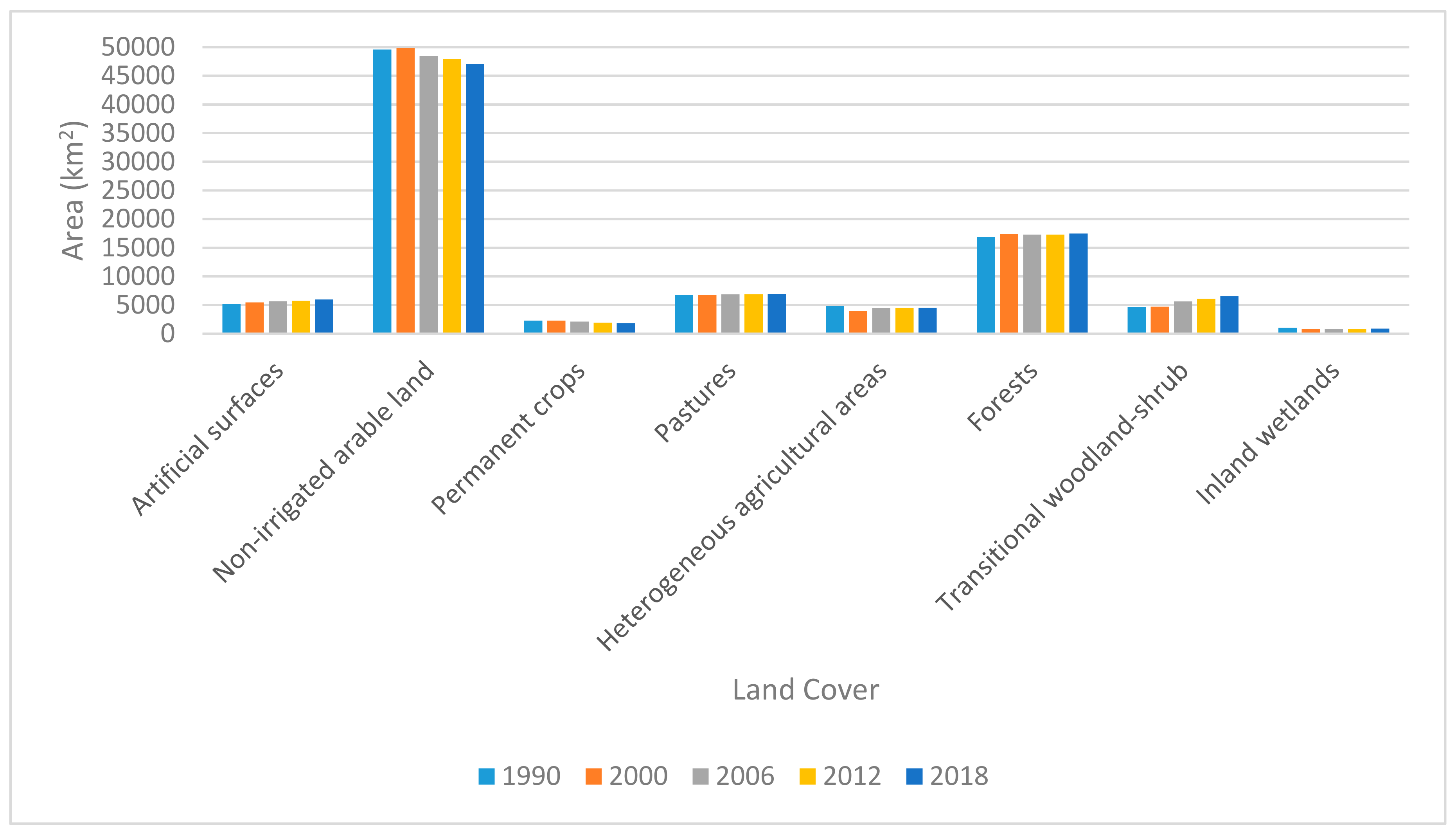
Information on LULC for the years 1990, 2000, 2006, 2012, and 2018 has been obtained from the respective CORINE Land Cover datasets at 100 × 100 m resolution.
The CORINE Land Cover (CLC) inventory includes 44 land cover classes for the abovementioned years. CLC mapping units are delineated via visual interpretation as well as by semi-automatic classification of satellite imagery. The geometric accuracy of the datasets is generally better than 100 m, while the thematic accuracy is typically above 85%, depending on countries [57].
All land use related layers for the PESERA model have been derived by the reclassification of the CORINE data based on the PESERA Manual [55]. As annual information on crops at arable land at a hectare level was not available, maize crop has been selected as a worst-case scenario for both the PESERA and the USLE (C factor) models, with an April sowing date. For the same reason, the USLE P factor has been set to 1, as detailed information was not available at a national scale.
C factor for the USLE model has been calculated based on the CLC values according to Podmaniczky et al. [61]

2.3.2. Climatic Information

The year 2010 has been selected as a baseline for comparing the effects of LULC changes. Therefore, all LULC “scenarios” have used the same climatic input variables. Where available, climate data was obtained from the CARPATCLIM database [3]. However, since a part of western Hungary is not covered by CARPATCLIM, AGRI4CAST MARS data [58] has been used to supplement it. The two datasets have been merged and re-interpolated for a 100 m grid via Ordinary Kriging in SAGA GIS. The PESERA model used monthly data (precipitation, PET, and temperature), while the USLE only required yearly precipitation data, where the extreme nature of the 2010 precipitation was represented as a 20-years return frequency. Calculation of R was based on the method proposed by Renard and Freimund [62], by the combined use of the following equations:
R = 0.04830   P 1.610
and
R = 587.8 1.219   P + 0.004105   P 2
where P is the mean annual precipitation. Equation (3) has been applied where P < 850 mm, while Equation (4) has been applied for P > 850 mm.

2.3.3. Topography

Elevation-based characteristics for both models have been derived from the EU-DEM dataset [59]. The Standard deviation of elevation within 1.5 km radius (for PESERA) was calculated in ArcMap 10.1. The USLE L (slope length) and S (slope gradient) factor was calculated in SAGA GIS based on Moore’s method [63], according to the following equation:
L S =   0.4 + 1 A s 22.13 0.4 sin β 0.0896 1.3
where β is the average slope and As is the specific catchment area.

2.3.4. Soil Information

Soil parameters (particle size distribution, organic matter content and carbonate content) have been provided from the DOSoReMI.hu initiative [60], based on the Digital Kreybig Soil Information System (DKSIS) [64] and the Hungarian Soil Information and Monitoring System [65]. The USLE K factor has been calculated based on the method of Sharply and Williams [66]:
K =   0.2 + 0.3 e 0.256 S A N 1 S I L / 100 × S I L C L A + S I L 0.3 × 1 0.25 O M O M + e 3.72 2.95 O M × 1 0.7 S N 1 S N 1 + e 22.9 S N 1 5.51
where SAN = sand, SIL = silt, CLA = clay and OM = organic matter content of the soil while SN1 = 1-SAN/100.
The PESERA soil erodibility and surface crusting factors were calculated based on Fryrear et al. [67], while soil water available to plants, effective soil water capacity, and scale depth have been downscaled from the original pan-European dataset [55], using regression kriging and conditional generalization [18].

2.4. Harmonization and Combination of Results

The applied harmonization/combination procedure followed the method, which had been used earlier in developing and evaluating the Soil Erosion Map of Hungary [18,22,
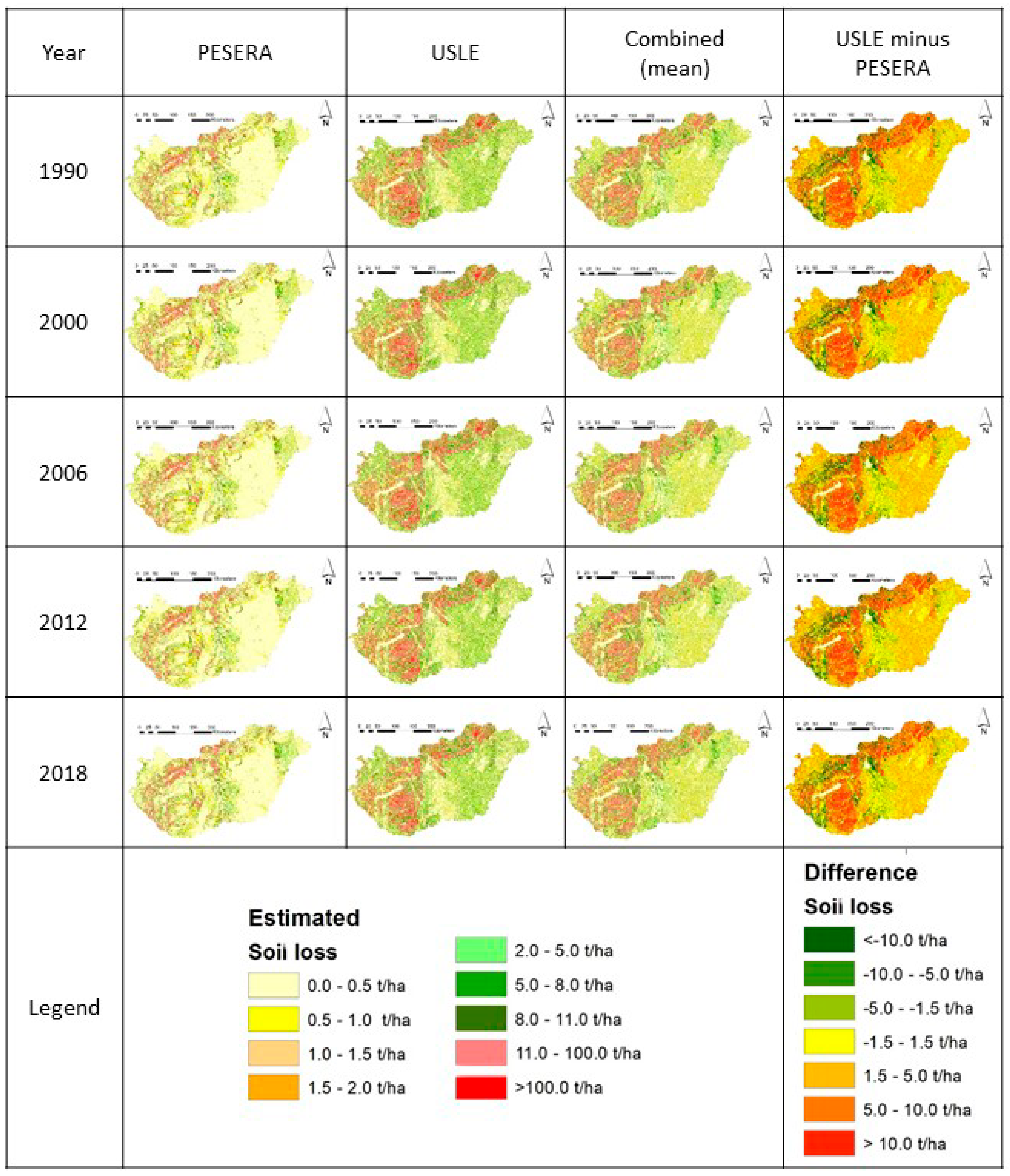
45]. Some predicted values proved to be negative. These values have resulted from the modeling process. In case of the USLE, they represent urban areas or waterbodies that were later masked out during the procedure and thus set to 0. As the PESERA model also calculates sediment accumulation, its negative values are actually meaningful. However, since sediment accumulation was not in the scope of the current study, in order to avoid any confusing results, predicted values below 0 have been set to 0. This does not affect the results, as soil erosion in deposition sites is considered zero.
The combination of outputs from the two models involved calculating a cell-by-cell mean of the two model outputs. Where only one of the models produced outputs (due to slight differences in methodology), the existing results were accepted.

2.5. Evaluation and Analysis

Statistical analysis of the results primarily included basic descriptive analysis and cross-correlation tables. Year to year comparison of erosion estimates followed the general rule of subtracting the output of the earlier scenario later one. This produced positive values where values have increased and negative ones where they decreased. Comparison of the USLE and PESERA outputs was carried out by calculating the difference between the two output layers for each modeled year.
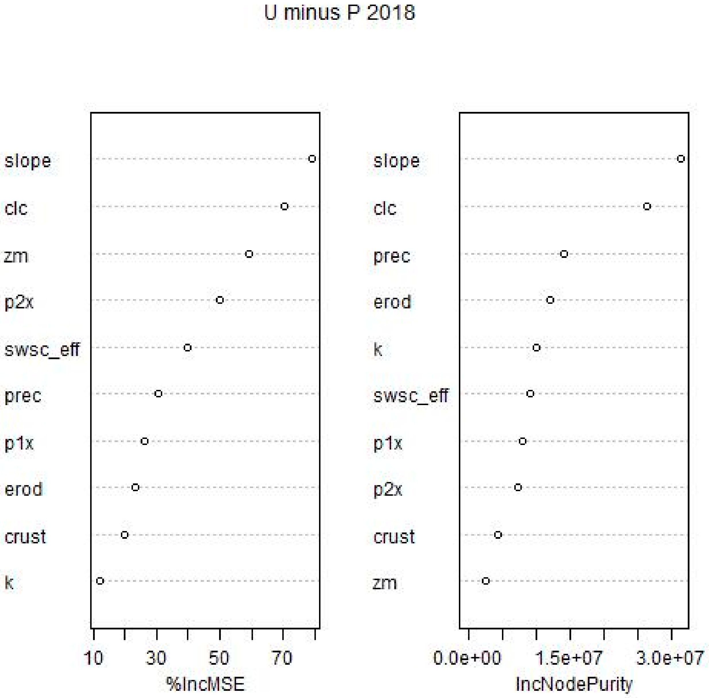
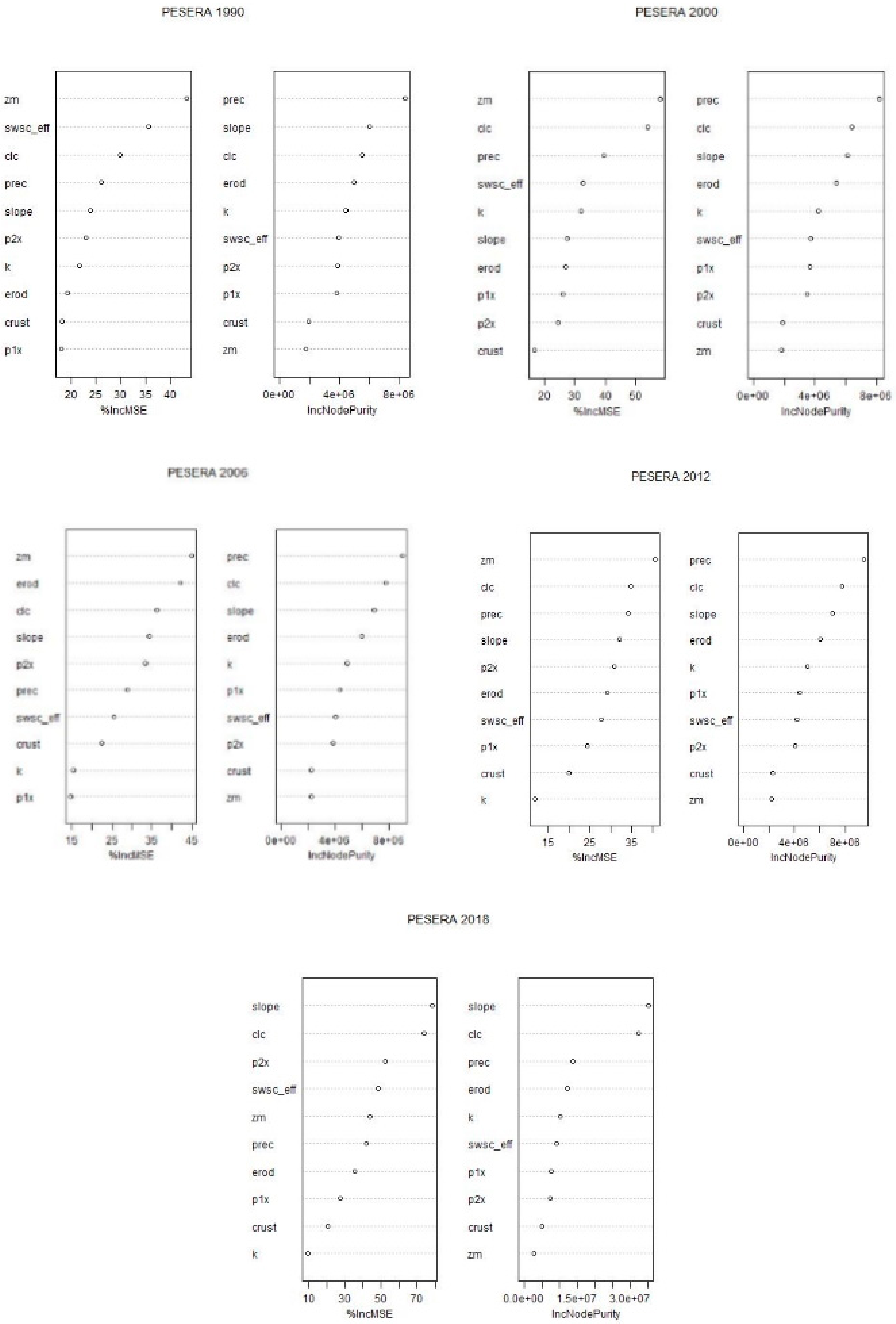
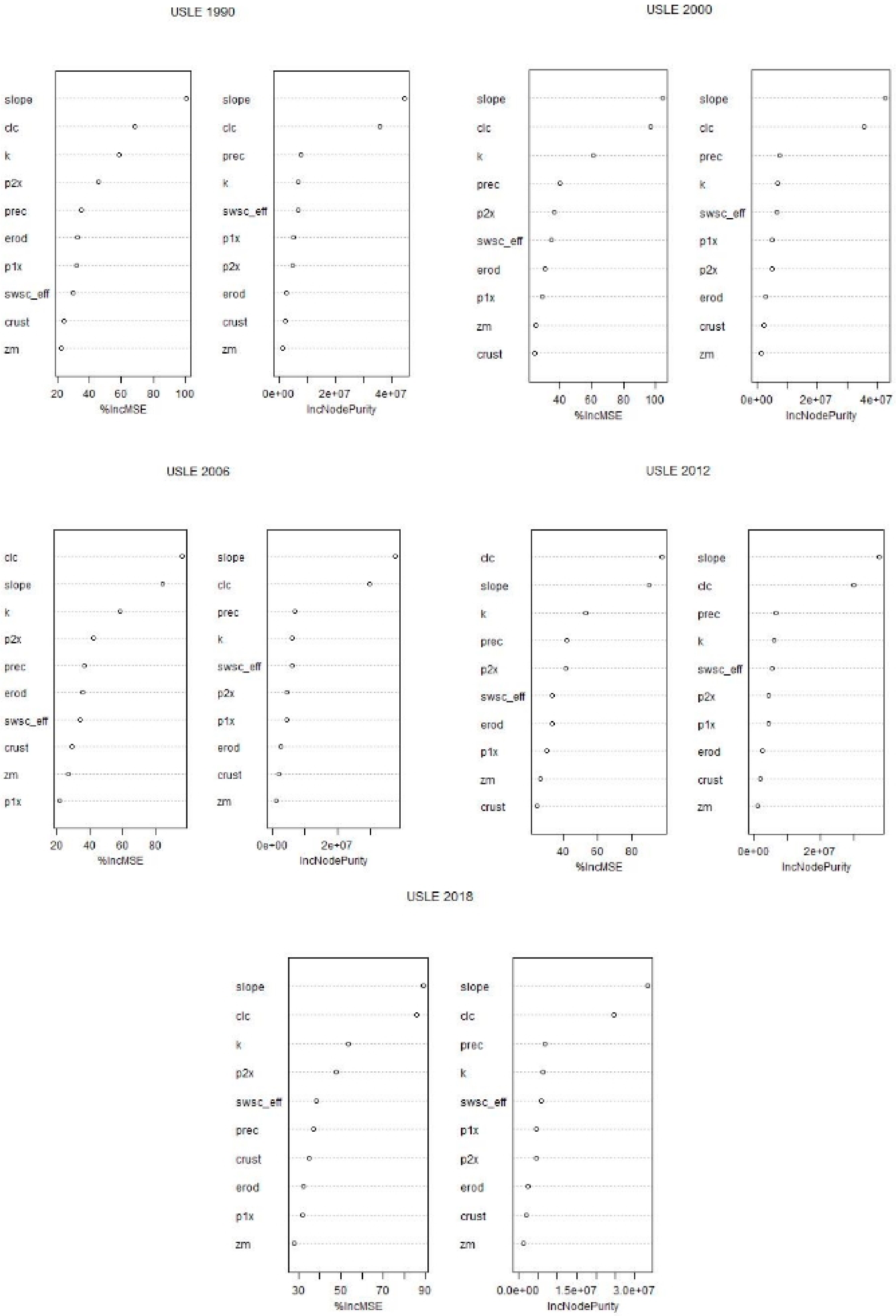
In order to assess the influence of different input variables, Random Forest regression models have been created for each modeled year, for both models as well as the differences in the predicted results of the two model, from a randomized representative subsample of 70,236 points, using the randomForest package in R. For each model, 500 regression trees have been grown, with 3 variables tried at each node. Since the since the specific input variables were in many ways different between the two models, a set of 10 key variables have been identifies representing the potential effects of precipitation (total annual rainfall in 2010, “prec”), slope (‘slope’), land cover (CORINE Land Cover, “clc”) and soil properties (USLE K factor, “k”; PESERA crust storage, “crust”; PESERA sensitivity to erosion, “erod”; PESERA effective soil water storage capacity, “swsc_eff”; PESERA soil water available to plants in top 300 mm, “p×1”; PESERA soil water available to plants between 300 and 1000 mm, “p×2”; PESERA scale depth, “zm”).

3. Results

3.1. Land Cover Change

The identified changes in LULC are summarized in Figure 4, with original CORINE categories merged into major groups for better presentation. The figure shows an almost continuous reduction in “Non-irrigated arable land”, coupled with an increase of “Artificial surfaces” and “Transitional woodland-shrub”, while other categories seem to have only slight variations.
Figure 5 presents the changes as a percentage of the total area covered by each category. The most observable trends are the reduction of non-irrigated arable land and the increase of artificial surfaces and transitional woodland–shrub areas. These indicate that such changes are primarily driven by land use and natural succession can play a part only when arable land is (either temporarily or long term) not being cultivated. The changes are generally well-distributed in the country, and occur mostly sporadically, without any visible spatial trends at the national level. A summary of the changes from 1990 to 2018 is presented in Table 3, while more detailed comparison of all five years is presented in Appendix A.

3.2. Soil Erosion

As output of the erosion modeling and evaluation process, a total of 30 maps have been created (see Appendix B). Estimated soil loss maps have been prepared for the LULC distribution for the years 1990, 2000, 2006, 2012, and 2018. Results included PESERA and USLE based estimates as well as maps of the combined (mean) estimates.
Figure 6 presents the estimated soil loss based on the latest available (2018) land cover information based on the PESERA model. Output of the USLE model for the same year is presented in Figure 7, while the combined (mean) output is shown on Figure 8. Results for other years are provided in Appendix B (Figure A1 and Figure A2).
Spatial coverage of soil erosion classes showed no significant variation between the years. Most of the country area (PESERA: 83.7–83.6%; USLE: 63.6–65.1%) showed below 5 t/ha/y soil loss; while coverage of higher classes has varied between the two models for 5–10 t/ha/y (PESERA: 6.0–6.7%; USLE: 13.3–13.7%); and above 10 t/ha/y (PESERA: 10.3–10.7%; USLE: 21.6–22.7%).
In order to assess the effects of LULC changes and their spatial distribution, a number of maps have been created by subtracting predictions of the older map from the newer one. Changes in erosion rates from the year 1990 to 2018 are displayed in Figure 9, while changes for other years are presented in Appendix B.
Figure 10 presents the changes in mean soil loss over the observed time period for the different estimation (USLE, PESERA, combined) methods. The graphs clearly show that the effects of changes are more prominent in case of the USLE model, and thus the combined approach.
In order to evaluate the effect of land use on the prediction difference between the two models, Figure 11 displays the minimum and maximum values (thus also ranges) of prediction differences within CORINE categories. Some categories (211, 311, and 324) had higher variation than others. These results show that for certain classes (111—continuous urban fabric, 213—rice fields, 221—vineyards, 333—sparsely vegetated areas, 411—inland marshes, 511—water courses) USLE was more likely to provide higher estimates, while for other categories the over-/underestimation of the two methods were more balanced, with the possible exception of pastures (231), where PESERA was slightly more likely to produce higher estimates.
Table 4 presents the basic descriptive statistics on the effects of LULC changes. The mean shows that at a national level, with the exception of the period 1990 to 2000, the potential erosion has been continuously reduced.
Table 5 compares the changes estimated by the different methods. It clearly shows that the USLE method generally provided a higher mean estimate, while from 2000 onwards, the highest estimate was predicted by the PESERA method.
It has to be noted that the maximum values presented in most of this chapter are extremely high values that are not at all typical under Hungarian conditions. In fact, in all likelihood these extreme values are outliers. However, at present we have insufficient observed information to provide an appropriate baseline from which calculation and removal of extreme outliers would be possible. Observation of the spatial distribution of estimates above 100 t/ha/y indicate that these mostly occur in the hilly regions. In case of the PESERA, they mostly show up in the Transdanubian Mountains (north of Lake Balaton), while the USLE estimates are generally evenly distributed along the mountains/hills of Hungary.

3.3. Importance of Input Variables

In order to assess the importance of the input variables, affecting both the output of the models as well as the differences in predictions between the two, 15 Random Forest (RF) regression models have been calculated. Detailed results of these models are presented in Appendix C. An example visualization of variable importance for the differences between the two models for 2018 is presented on Figure 12. The left side of the figure indicates the importance of each variable as a percentage of increase in mean squared error (MSE) upon leaving out the variable, while the right-hand side presents node purity based on the Gini index.
The ranking of variables by importance is presented in Table 6. Table 7 presents the importance (see above) of each input variable, as well as the mean squared residuals and the % of variance explained by the Random Forest regression. It is important to note that the importance of these variables is presented based on the RF regression only, since the models themselves do not share the exact same input variables.

4. Discussion

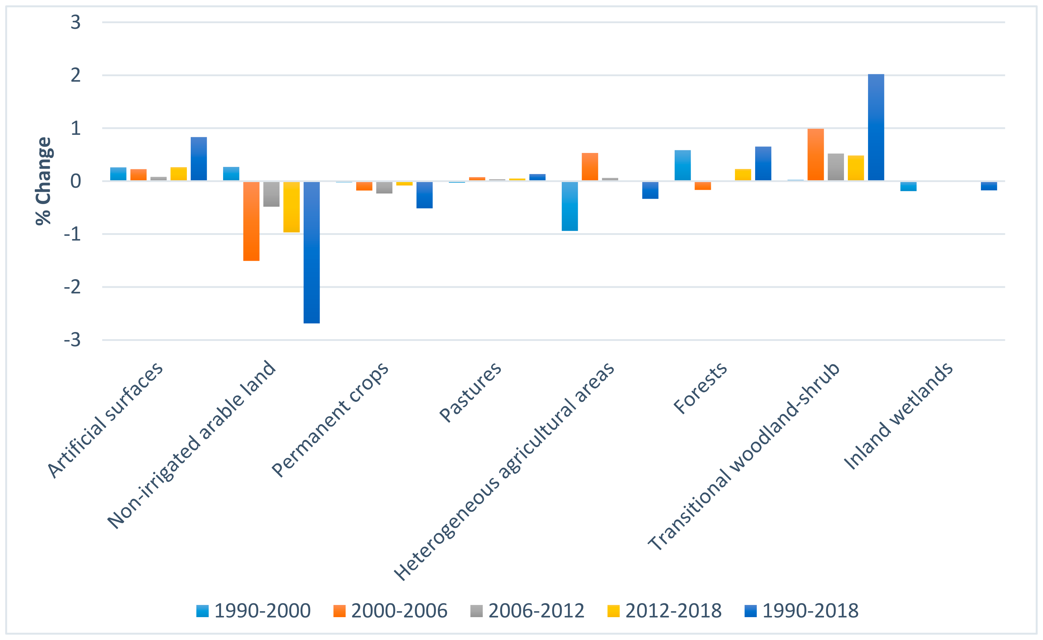
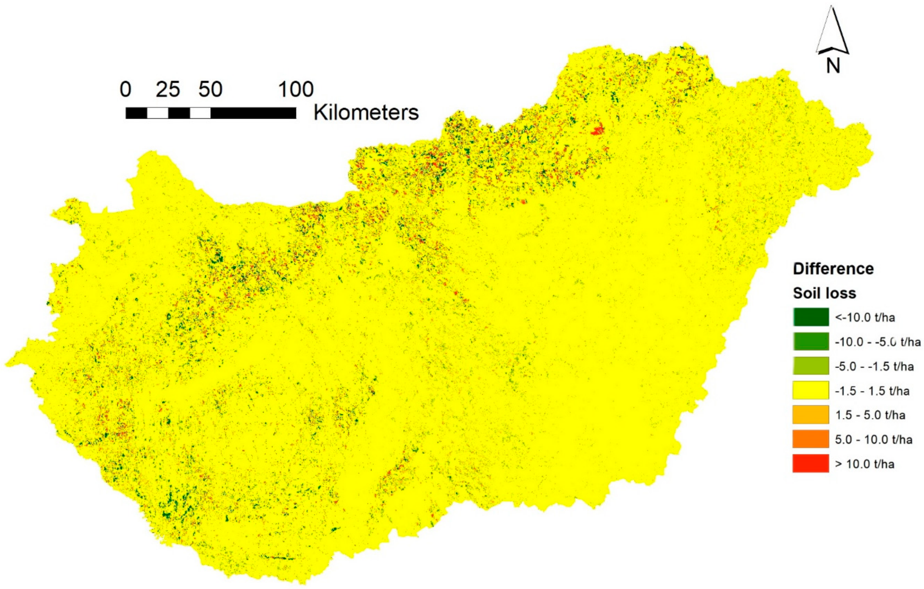
Analysis of the results have demonstrated that the effects of LULC changes between 1990 and 2018 are clearly present in Hungary, with a general reduction in soil erosion estimates. This indicates that the applied changes have somewhat reduced soil erosion risk in Hungary. Based on the comparison of estimated mean erosion values for the 1990 and the 2018 land cover, a reduction of 0.28 t/ha/year has been calculated. Considering the 93,030 km2 total territory of Hungary, this would mean the potential conservation of approximately 2.6 million tons of soil per year, under the same climatic conditions as 2010.
However, the spatial distribution of these changes is not even and it is clear that there are small areas all around the country where erosion risk has increased due to the changes in land cover. While the applied methodology of utilizing the CORINE datasets as input is well established [29], it is best applied for analyzing long-term changes. However, the same methodology could also be utilized to evaluate short-term changes based on Sentinel-2 imagery as demonstrated by Karydas et al. [68].
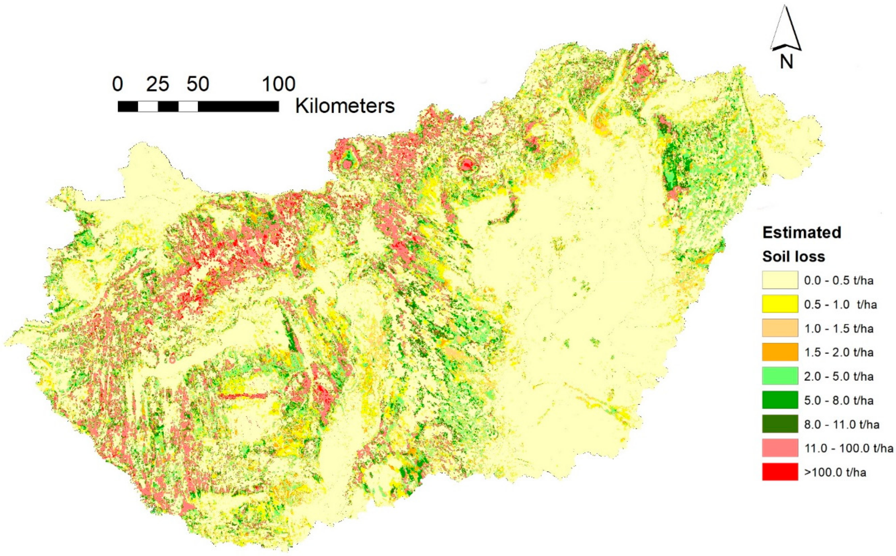
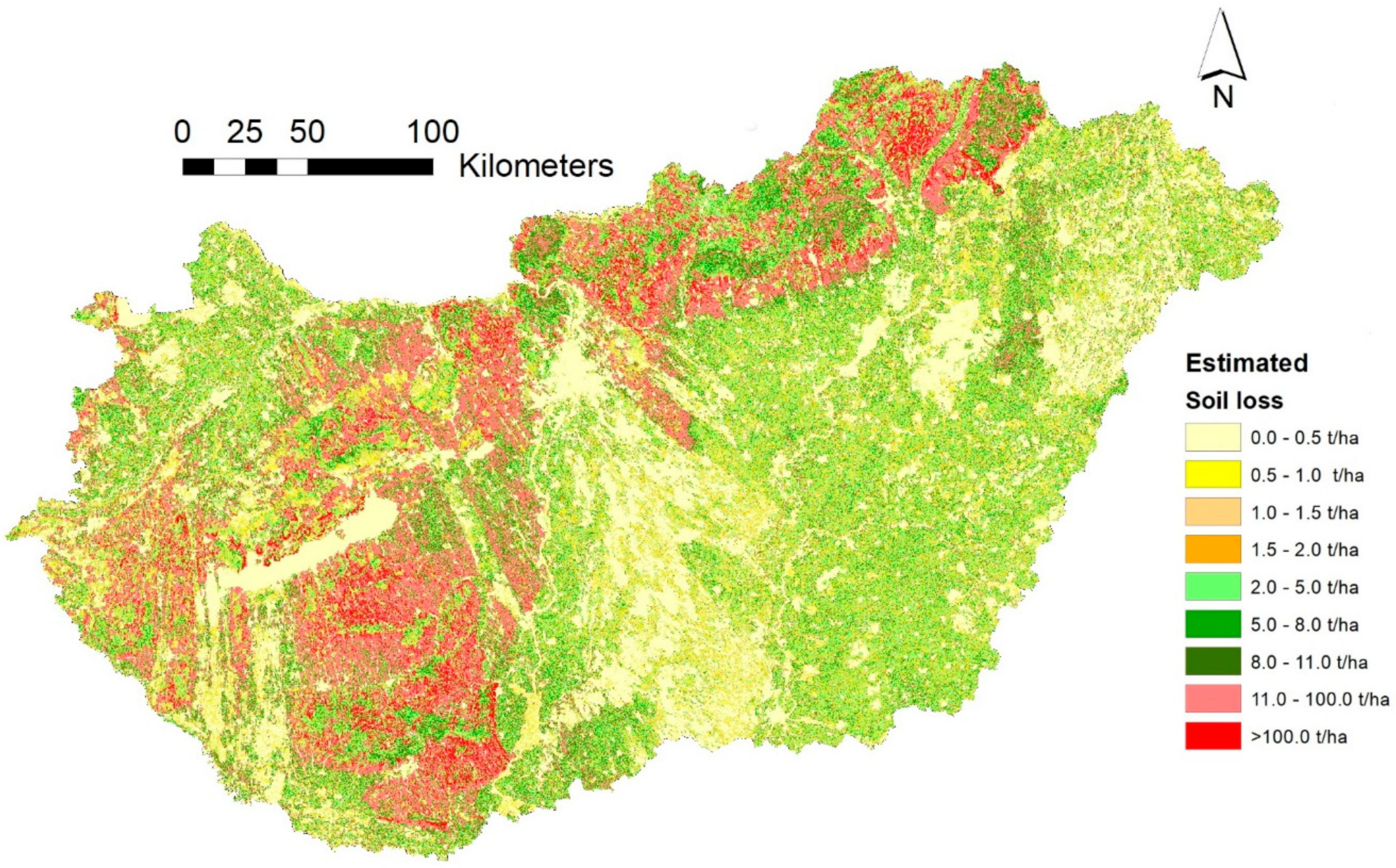
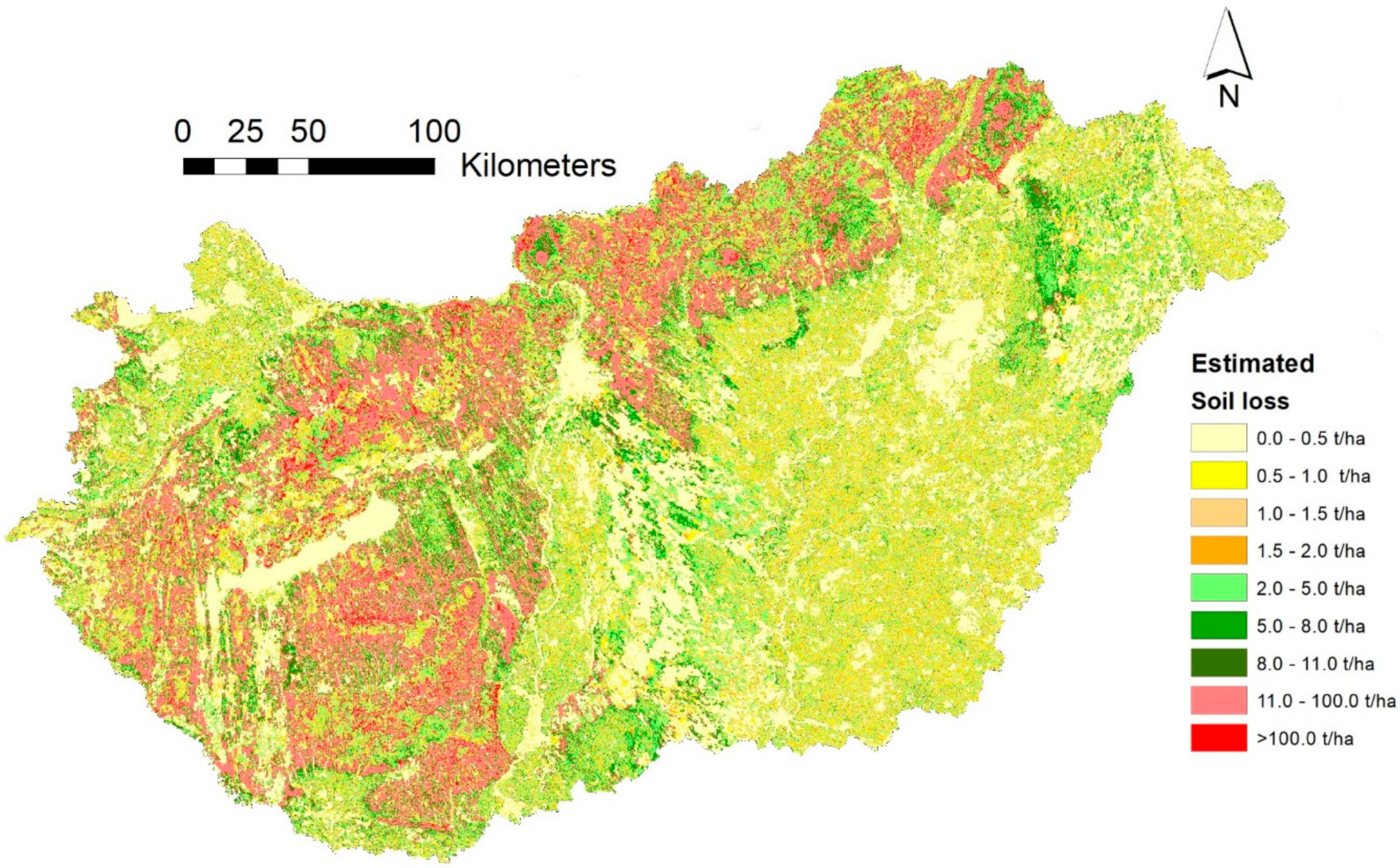
Spatial pattern of changes (Figure 9) in predicted erosion rates reveal that the effect of LULC changes are present throughout the country. However, visual interpretation of the results also suggests that the effect of these changes is much more significant in hilly and mountainous regions. This effect is clearly visible in (but not limited to) the North Hungarian Mountains and the Transdanubian Mountains. Occurrence as well as intensity of such changes (as variables influencing soil erosion) is less expressed in the low-lying areas, such as the Hungarian Great Plain.
The successful application of the two models supported the validity of their application as found in similar studies recently [69]. However, longer, more demanding processing for the PESERA model indicates the growing demand for higher level processing utilities, such as parallel processing capabilities for physically based models [70].
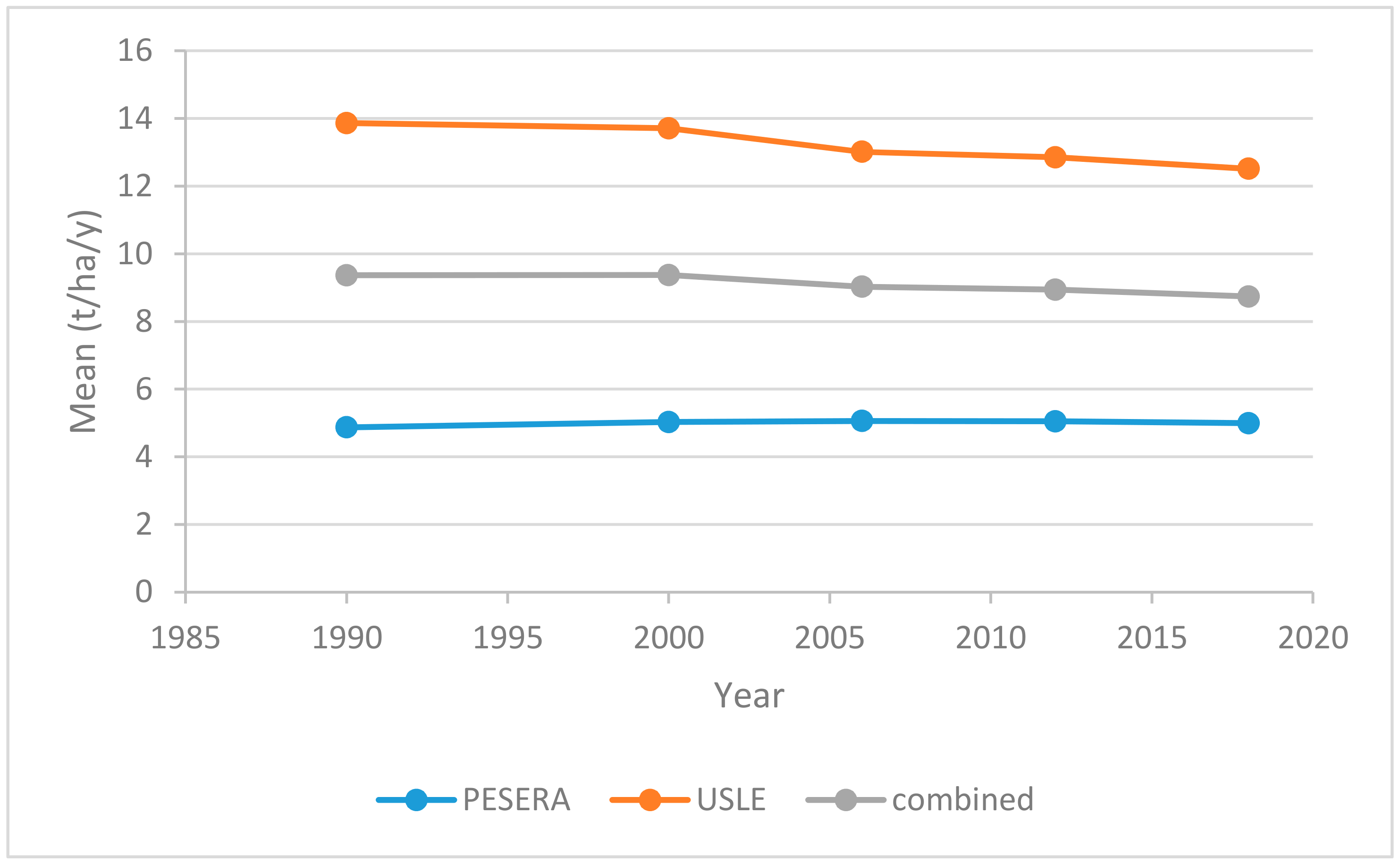
Comparison of the two models showed that as in previous studies, the USLE model produced generally higher estimates than the PESERA. This is in line with the findings of other studies [40,41,70] where applying the RUSLE and the PESERA model provided similar results. Their findings indicate that PESERA has performed better responding to changes in vegetation rather than to slope. Evaluation of the Random Forest regression analysis has confirmed this. It is also worth noting that PESERA was also more sensitive to soil parameters than the USLE model. The PESERA model is also likely to produce lower predictions at finer spatial resolutions [
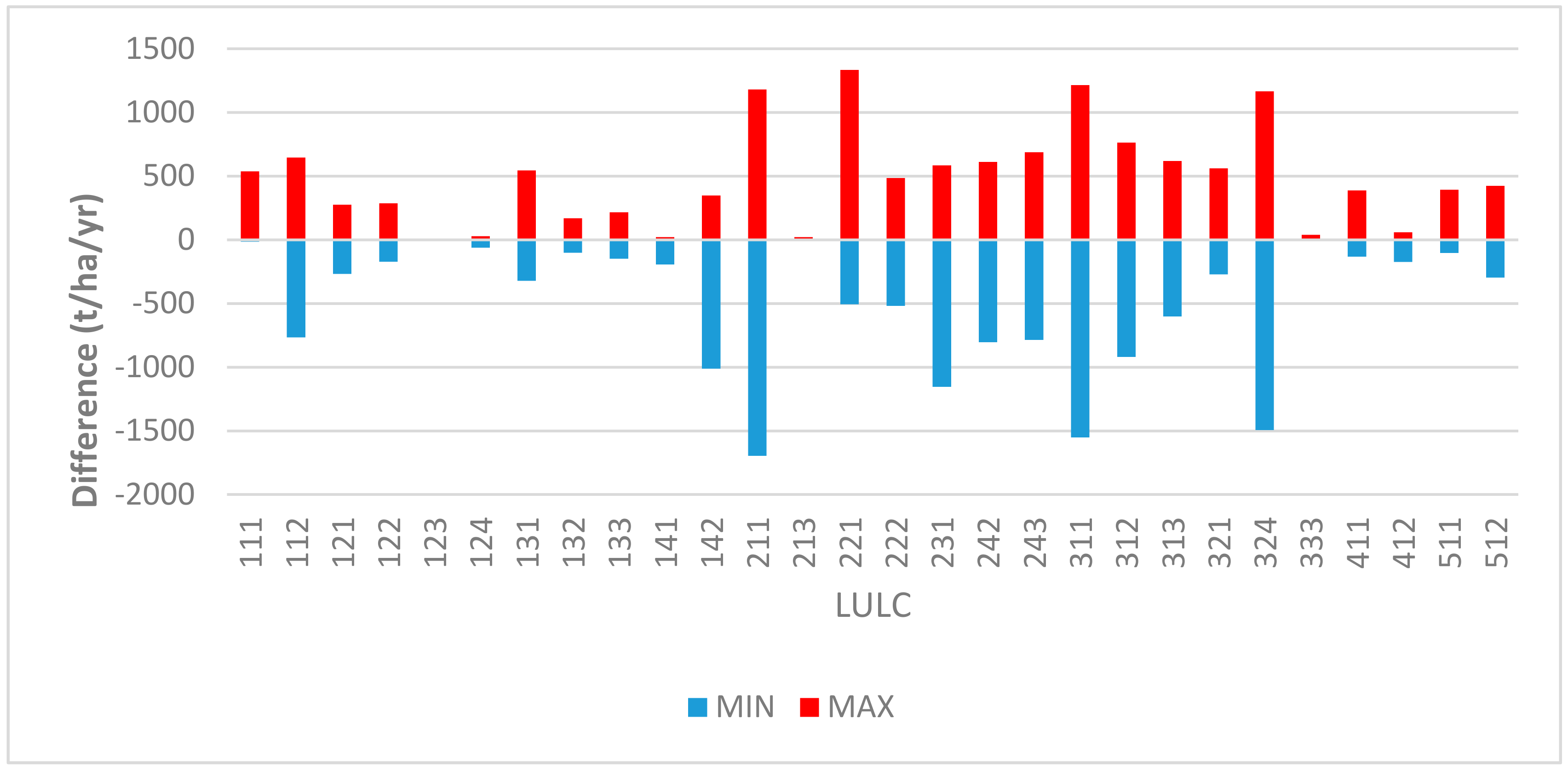
41], which clearly demonstrated its limitations when applying at smaller scales. Changes in the mean maximum values of the PESERA model have been less influenced by the land cover changes, indicating that the USLE model was more sensitive to such effects. The differences in predictions do not seem to be specific for any particular LULC classes. While some land cover categories indeed produced higher variations in prediction difference, these categories can also be associated with a higher spatial coverage. Table 6 and Table 7 indicate that the differences between the two model are mainly driven by their sensitivity to slope and land cover, followed by soil parameters. The differences in predictions underline the findings of [6] regarding the importance of communicating uncertainty in erosion models. While the existence of new and updated spatially explicit erosion estimates is undeniably beneficial, end users—including decision makers and the general public—should also be more aware of the limitations of these products.
Future research should focus on the appropriate determination method for outlier predictions and their removal from the datasets. A comparison of model estimates with field-based monitoring data would also be invaluable for a proper valuation of the methodologies.

5. Conclusions

During our research, we have successfully applied a combined approach of the PESERA and USLE models for estimating the effects of recent LULC changes in Hungary. Based on our results and discussion above, we can establish the following conclusions:
  • Changes in land use/land cover from 1990 to 2018 have reduced potential soil erosion by water in Hungary by up to 0.28 t/ha/year on average.
  • LULC changes in Hungary have primarily affected the extent of non-irrigated arable land (decreased), artificial surfaces and transitional woodland-shrub areas (increased).
  • The USLE model generally provided higher estimates, with higher sensitivity to slope and to LULC changes.
  • The PESERA models has proven to be more sensitive to soil parameters.
As our results have indicated, the identification of outlier (extreme) predicted values are a critical issue and further analysis should be carried out to properly identify these. While our study has provided a combined approach for the use of the two models, the methodology could still be advanced by a potential implementation of spatially differential weighting based on the strengths/weaknesses of the applied models.

Author Contributions

Conceptualization, István Waltner and László Pásztor; data curation, Sahar Saeidi and János Grósz; formal analysis, Sahar Saeidi, Annamária Laborczi, and János Grósz; funding acquisition, István Waltner and László Pásztor; investigation, István Waltner, Sahar Saeidi, and János Grósz; methodology, István Waltner, Sahar Saeidi, and László Pásztor; project administration, István Waltner and László Pásztor; resources, István Waltner and János Grósz; supervision, István Waltner, Csaba Centeri, and László Pásztor; validation, János Grósz, Csaba Centeri, Annamária Laborczi, and László Pásztor; visualization, István Waltner and Sahar Saeidi; writing—original draft, István Waltner and Sahar Saeidi; writing—review and editing, János Grósz, Csaba Centeri, and László Pásztor. All authors have read and agreed to the published version of the manuscript.

Funding

Our work has been supported by the National Research, Development and Innovation Office [NKFIH; Grant No. KH-126725] and the Higher Education Institutional Excellence Program [NKFIH, Grant nos. 1150-6/2019 and 1159-6/2019]. This publication was supported by the EFOP-3.6.1-16-2016-0016 project: improvement of the research and training profile of the SZIU Campus in Szarvas in the themes of water management, hydroculture, precision mechanical engineering, alternative crop production.

Acknowledgments

The authors would like to thank Zoltán Vekerdy for his support in the initial conceptualization of the project.

Conflicts of Interest

The authors declare no conflict of interest. The funders had no role in the design of the study; in the collection, analyses, or interpretation of data; in the writing of the manuscript, or in the decision to publish the results.

Appendix A

Land Use and Land Cover change tables for Hungary based on CORINE Land Cover data.
Table A1. Area affected by LULC change in Hungary between 1990 and 2000.
LULC 1990–20001990 (ha)2000 (ha)Changes (ha)Changes %
Urban fabric415,567427,64112,0740.13
Industrial, commercial, transport56,84863,98271340.08
Mine, dump and construction sites11,86913,57317040.02
Green urban areas, sport-leisure facilities36,37339,58132080.03
Non-irrigated arable land4,958,9004,983,92125,0210.27
Rice fields14,77511,786–2989–0.03
Permanent crops215,013215,9859720.01
Pastures680,005677,439–2566–0.03
Heterogeneous agricultural areas483,859396,449–87,410–0.94
Forests1,684,2941,738,78554,4910.59
Natural grasslands225,809228,46326540.03
Transitional woodland-shrub241,934241,691–243–0.00
Sparsely vegetated areas24132330–83–0.00
Inland wetlands103,42885,875–17,553–0.19
Inland waters170,175173,76135860.04
Table A2. Area affected by LULC change in Hungary between 2000 and 2006.
LULC 2000–20062000 (ha)2006 (ha)Changes (ha)Changes (%)
Urban fabric427,641435,08174400.08
Industrial, commercial, transport63,98271,03370510.08
Mine, dump, and construction sites13,57320,46268890.07
Green urban areas, sport-leisure facilities39,58139,406–175–0.00
Non-irrigated arable land4,983,9214,843,860–140,061–1.51
Rice fields11,78611,169–617–0.01
Permanent crops215,985200,256–15,729–0.17
Pastures677,439684,33368940.07
Heterogeneous agricultural areas396,449445,89349,4440.53
Forests1,738,7851,723,106–15,679–0.17
Natural grasslands228,463228,308–155–0.00
Transitional woodland-shrub241,691333,84092,1490.99
Sparsely vegetated areas233027033730.00
Inland wetlands85,87586,0401650.00
Inland waters173,761175,77220110.02
Table A3. Area affected by LULC change in Hungary between 2006 and 2012.
LULC 2006–20122006 (ha)2012 (ha)Changes (ha)Changes (%)
Urban fabric435,081438,74936680.04
Industrial, commercial, transport71,03377,59865650.07
Mine, dump, and construction sites20,46217,416–3046–0.03
Green urban areas, sport-leisure facilities39,40639,8524460.00
Non-irrigated arable land4,843,8604,799,046–44,814–0.48
Rice fields11,1698247–2922–0.03
Permanent crops200,256181,391–18,865–0.20
Pastures684,333687,65733240.04
Heterogeneous agricultural areas445,893451,72558320.06
Forests1,723,1061,723,3192130.00
Natural grasslands228,308228,6653570.00
Transitional woodland-shrub333,840382,06948,2290.52
Sparsely vegetated areas2703270300.00
Inland wetlands86,04086,04330.00
Inland waters175,772176,78210100.01
Table A4. Area affected by LULC change in Hungary between 2012 and 2018.
LULC 2012–20182012 (ha)2018 (ha)Changes (ha)Changes (%)
Urban fabric438,749452,28313,5340.15
Industrial, commercial, transport77,59889,02711,4290.12
Mine, dump, and construction sites17,41616,489–927–0.01
Green urban areas, sport-leisure facilities39,85240,3795270.01
Non-irrigated arable land4,799,0464,708,948–90,098–0.97
Rice fields82478048–199–0.00
Permanent crops181,391174,079–7312–0.08
Pastures687,657692,42147640.05
Heterogeneous agricultural areas451,725452,7069810.01
Forests1,723,3191,744,54621,2270.23
Natural grasslands228,665230,78621210.02
Transitional woodland-shrub382,069425,02742,9580.46
Sparsely vegetated areas270328441410.00
Inland wetlands86,04387,16211190.01
Inland waters176,782176,579–203–0.00

Appendix B

Soil erosion estimates and changes.
Figure A1. Erosion estimates for the observed years and applied methods.
Ijgi 09 00667 g0a1
Figure A2. Changes in erosion estimates between the observed years (PESERA and USLE models combined).
Ijgi 09 00667 g0a2

Appendix C

Detailed results of Random Forest regression analysis.
Importance of variables is presented by analyzed method (P—PESERA; U—USLE; %IncMSE—percentage of increase in MSE; prec—total annual rainfall in 2010; slope—slope; clc—CORINE Land Cover; k—USLE K factor; crust—PESERA crust storage; erod—PESERA sensitivity to erosion; swsc_eff—PESERA effective soil water storage capacity; p×1. PESERA soil water available to plants in top 300 mm; p×2—PESERA soil water available to plants between 300 and 1000 mm; zm—PESERA scale depth). The left side of the figure indicates the importance of each variable as a percentage of increase in mean squared error (MSE) upon leaving out the variable, while the right-hand side presents node purity based on the Gini index.
Figure A3. Variable importance based on Random Forest regression for PESERA model for all modeled years.
Ijgi 09 00667 g0a3
Figure A4. Variable importance based on Random Forest regression for the USLE model for all modeled years.
Ijgi 09 00667 g0a4
Figure A5. Variable importance based on Random Forest regression for the differences between the USLE (U) and PESERA (P) models for all modeled years.
Ijgi 09 00667 g0a5

References

  1. European Commission. Communication of 16 April 2002 from the Commission to the Council, the European Parliament, the Economic and Social Committee and the Committee of the Regions: Towards a Thematic Strategy for Soil Protection; European Commission: Brussels, Belgium, 2002. [Google Scholar]
  2. Van den Besselaar, E.J.M.; Klein Tank, A.M.G.; Buishand, T.A. Trends in European precipitation extremes over 1951–2010. Int. J. Climatol. 2013. [Google Scholar] [CrossRef]
  3. Szalai, S.; Auer, I.; Hiebl, J.; Milkovich, J.; Radim, T.; Stepanek, P.; Zahradnicek, P.; Bihari, Z.; Lakatos, M.; Szentimrey, T.; et al. Climate of the Greater Carpathian Region. Final Technical Report. 2013. Available online: www.carpatclim-eu.org (accessed on 2 October 2020).
  4. Panagos, P.; Katsoyiannis, A. Soil erosion modelling: The new challenges as the result of policy developments in Europe. Envres 2019, 172, 470–474. [Google Scholar] [CrossRef] [PubMed]
  5. Li, P.; Zang, Y.; Ma, D.; Yao, W.; Holden, J.; Irvine, B.; Zhao, G. Soil erosion rates assessed by RUSLE and PESERA for a Chinese Loess Plateau catchment under land-cover changes. Earth Surf. Process. Landf. 2020, 45, 707–722. [Google Scholar] [CrossRef]
  6. Batista, P.V.; Davies, J.; Silva, M.L.; Quinton, J.N. On the evaluation of soil erosion models: Are we doing enough? Earth-Sci. Rev. 2019, 197, 102898. [Google Scholar] [CrossRef]
  7. Wischmeier, W.H.; Smith, D.D. Predicting Rainfall Erosion Losses: A Guide to Conservation Planning Science; US Department of Agriculture Handbook: Washington, DC, USA, 1978; p. 537.
  8. Sadeghi, S.H.; Mizuyama, T.; Miyata, S.; Gomi, T.; Kosugi, K.; Mizugaki, S.; Onda, Y. Is MUSLE apt to small steeply reforested watershed? J. For. Res. 2007, 12, 270–277. [Google Scholar] [CrossRef]
  9. Odongo, V.O.; Onyando, J.O.; Mutua, B.M.; van Oel, P.R.; Becht, R. Sensitivity analysis and calibration of the Modified Universal Soil Loss Equation (MUSLE) for the upper Malewa Catchment, Kenya. Int. J. Sediment. Res. 2013, 28, 368–383. [Google Scholar] [CrossRef]
  10. Conforti, M.; Buttafuocoa, G.; Ragob, V.; Aucellic, P.P.C.; Robustellib, G.; Scarciglia, F. Soil loss assessment in the Turbolo catchment (Calabria, Italy). J. Maps 2015, 12, 815–825. [Google Scholar] [CrossRef]
  11. Minaei, M.; Kainz, W. Watershed Land Cover/Land Use Mapping Using Remote Sensing and Data Mining in Gorganrood, Iran. Isprs Int. J. Geo-Inf. 2016, 5, 57. [Google Scholar] [CrossRef] [Green Version]
  12. Zhang, K.; Yu, Y.; Dong, J.; Yang, Q.; Xu, X. Adapting & testing use of USLE K factor for agricultural soils in China. Agric. Ecosyst. Environ. 2019, 269, 148–155, ISSN 0167-8809. [Google Scholar] [CrossRef]
  13. Srinivasan, R.; Singh, S.K.; Nayak, D.C.; Hegde, R.; Ramesh, M. Estimation of soil loss by USLE Model using Remote Sensing and GIS Techniques-A Case study of Coastal Odisha, India. Eurasian J. Soil Sci. 2019, 8, 321–328. [Google Scholar] [CrossRef]
  14. Borrelli, P.; Meusburger, K.; Ballabio, C.; Panagos, P.; Alewell, C. Object-oriented soil erosion modelling: A possible paradigm shift from potential to actual risk assessments in agricultural environments. Land Degrad Dev. 2018, 29, 1270–1281. [Google Scholar] [CrossRef]
  15. Phinzi, K.; Abriha, D.; Bertalan, L.; Holb, I.; Szabó, S. Machine Learning for Gully Feature Extraction Based on a Pan-Sharpened Multispectral Image: Multiclass vs. Binary Approach. Isprs Int. J. Geo-Inf. 2020, 9, 252. [Google Scholar] [CrossRef] [Green Version]
  16. Stefanovits, P. Soil Degradation in Hungary; OMMI: Budapest, Hungary, 1964. (In Hungarian) [Google Scholar]
  17. Centeri, C.S.; Pataki, R. Erosion map of Hungary. In Proceedings of the Conference on Environmental Management of the Rural Landscape in Central and Eastern Europe, Podbanske, Slovakia, 2–6 September 2000; pp. 20–22. [Google Scholar]
  18. Pásztor, L.; Waltner, I.; Centeri, C.; Belényesi, M.; Takács, K. Soil erosion of Hungary assessed by spatially explicit modelling. J. Maps 2016, 12, 407–414. [Google Scholar] [CrossRef] [Green Version]
  19. Kocsis, K. (Editor-in-chief); National Atlas of Hungary: Natural Environment; Hungarian Academy of Sciences, Research Centre for Astronomy and Earth Sciences, Geographical Institute: Budapest, Hungary, 2018; ISBN 978-963-9545-57-1. [Google Scholar]
  20. Bartus, M.; Barta, K.; Szatmári, J.; Farsang, A. Csongrád megye talajainak szélcsatorna kísérletekre alapozott szélerózió veszélyeztetettség becslése. Agrokémia És Talajt. 2019, 68, 225–242. [Google Scholar] [CrossRef]
  21. Kertész, A.; Centeri, C.S. Soil Erosion in Europe; Boardman, J., Poesen, J., Eds.; John Wiley & Sons: Chichester, UK, 2006. [Google Scholar]
  22. Waltner, I.; Pásztor, L.; Centeri, C.; Takács, K.; Pirkó, B.; Koós, S.; László, P. Evaluating the new soil erosion map of Hungary—A semiquantitative approach. Land Degrad Dev. 2018, 29, 1295–1302. [Google Scholar] [CrossRef]
  23. Keller, B.; Szabó, J.; Centeri, C.; Jakab, G.; Szalai, Z. Different land-use intensities and their susceptibility to soil erosion. Agrokémia És Talajt. 2019, 68, 14–23. [Google Scholar] [CrossRef]
  24. Rubio-Delgado, J.; Schnabel, S.; Gómez-Gutiérrez, Á.; Lavado-Contador, J.F. Temporal and spatial variation of soil erosion in wooded rangelands of southwest Spain. Earth Surf. Process. Landf. 2019, 44, 2141–2155. [Google Scholar] [CrossRef]
  25. Guo, Y.; Peng, C.; Zhu, Q.; Wang, M.; Wang, H.; Peng, S.; He, H. Modelling the impacts of climate and land use changes on soil water erosion: Model applications, limitations and future challenges. J. Environ. Manag. 2019, 250, 109403. [Google Scholar] [CrossRef]
  26. Yeshaneh, E.; Wagner, W.; Exner-Kittridge, M.; Legesse, D.; Blöschl, G. Identifying Land Use/Cover Dynamics in the Koga Catchment, Ethiopia, from Multi-Scale Data, and Implications for Environmental Change. Isprs Int. J. Geo-Inf. 2013, 2, 302–323. [Google Scholar] [CrossRef] [Green Version]
  27. Kijowska-Strugała, M.; Bucała-Hrabia, A.; Demczuk, P. Long-term impact of land use changes on soil erosion in an agricultural catchment (in the Western Polish Carpathians). Land Degrad. Dev. 2018, 29, 1871–1884. [Google Scholar] [CrossRef]
  28. Bonetti, S.; Richter, D.D.; Porporato, A. The effect of accelerated soil erosion on hillslope morphology. Earth Surf. Process. Landf. 2019, 44, 3007–3019. [Google Scholar] [CrossRef]
  29. Borrelli, P.; Van Oost, K.; Meusburger, K.; Alewell, C.; Lugato, E.; Panagos, P. A step towards a holistic assessment of soil degradation in Europe: Coupling on-site erosion with sediment transfer and carbon fluxes. Environ. Res. 2018, 161, 291–298. [Google Scholar] [CrossRef]
  30. Raclot, D.; Le Bissonnais, Y.; Annabi, M.; Sabir, M.; Smetanova, A. Main Issues for Preserving Mediterranean Soil Resources from Water Erosion Under Global Change. Land Degrad. Dev. 2018, 29, 789–799. [Google Scholar] [CrossRef]
  31. Fayas, C.M.; Abeysingha, N.S.; Nirmanee, K.G.S.; Samaratunga, D.; Mallawatantri, A. Soil loss estimation using RUSLE model to prioritize erosion control in KELANI river basin in Sri Lanka. Int. Soil Water Conserv. Res. 2019, 7, 130–137. [Google Scholar] [CrossRef]
  32. Boluwade, A. Regionalization and Partitioning of Soil Health Indicators for Nigeria Using Spatially Contiguous Clustering for Economic and Social-Cultural Developments. Isprs Int. J. Geo-Inf. 2019, 8, 458. [Google Scholar] [CrossRef] [Green Version]
  33. Yu, H.; Wang, L.; Wang, Z.; Ren, C.; Zhang, B. Using Landsat OLI and Random Forest to Assess Grassland Degradation with Aboveground Net Primary Production and Electrical Conductivity Data. Isprs Int. J. Geo-Inf. 2019, 8, 511. [Google Scholar] [CrossRef] [Green Version]
  34. Shrestha, S.; Bhatta, B.; Shrestha, M.; Shrestha, P.K. Integrated assessment of the climate and landuse change impact on hydrology and water quality in the Songkhram River Basin, Thailand. Sci. Total Environ. 2018, 643, 1610–1622. [Google Scholar] [CrossRef]
  35. Zhang, L.; Nan, Z.; Xu, Y.; Li, S. Hydrological impacts of land use change and climate variability in the headwater region of the Heihe River Basin, Northwest China. PLoS ONE 2016, 11. [Google Scholar] [CrossRef]
  36. Lamichhane, S.; Shakya, N.M. Integrated Assessment of Climate Change and Land Use Change Impacts on Hydrology in the Kathmandu Valley Watershed, Central Nepal. Water 2019, 11, 2059. [Google Scholar] [CrossRef] [Green Version]
  37. Aghsaei, H.; Dinan, N.M.; Moridi, A.; Asadolahi, Z.; Delavar, M.; Fohrer, N.; Wagner, P.D. Effects of dynamic land use/land cover change on water resources and sediment yield in the Anzali wetland catchment, Gilan, Iran. Sci. Total Environ. 2020, 712, 136–449. [Google Scholar] [CrossRef] [PubMed]
  38. Burns, P.; Nolin, A. Using atmospherically-corrected Landsat imagery to measure glacier area change in the cordillera Blanca, Peru from 1987 to 2010. Remote Sens. Environ. 2014, 140, 165–178. [Google Scholar] [CrossRef] [Green Version]
  39. Chemura, A.; Rwasoka, D.; Mutanga, O.; Dube, T.; Mushore, T. The impact of land-use/land cover changes on water balance of the heterogeneous Buzi sub-catchment, Zimbabwe. Remote Sens. Appl. Soc. Environ. 2020, 18, 100292. [Google Scholar] [CrossRef]
  40. Fernández, C.; Vega, J.A. Evaluation of RUSLE and PESERA models for predicting soil erosion losses in the first year after wildfire in NW Spain. Geoderma 2016, 273, 64–72. [Google Scholar] [CrossRef]
  41. Baggaley, N.; Potts, J. Sensitivity of the PESERA soil erosion model to terrain and soil inputs. Geoderma Reg. 2017, 11, 104–112. [Google Scholar] [CrossRef]
  42. Ciampalini, R.; Constantine, J.A.; Walker-Springett, K.J.; Hales, T.C.; Ormerod, S.J.; Hall, I.R. Modelling soil erosion responses to climate change in three catchments of Great Britain. Sci. Total Environ. 2020, 749, 141657. [Google Scholar] [CrossRef] [PubMed]
  43. Archer, K.J.; Kimes, R.V. Empirical characterization of random forest variable importance measures. Comput. Stat. Data Anal. 2008, 52, 2249–2260. [Google Scholar] [CrossRef]
  44. Zhang, F.; Yang, X. Improving land cover classification in an urbanized coastal area by random forests: The role of variable selection. Remote Sens. Environ. 2020, 251, 112105. [Google Scholar] [CrossRef]
  45. Szabó, J.; Schweitzer, F.; Horváth, G.; Bihari, Z.; Czigány, S.Z.; Fábián, S.Z.; Gábris, G.Y.; Iványi, K.; Kerényi, A.; Lóki, J.; et al. Natural Hazards; Kocsis, K., Ed.; Hungarian Academy of Sciences, Research Centre for Astronomy and Earth Sciences, Geographical Institute: Budapest, Hungary, 2018; pp. 156–167. ISBN 978-963-9545-57-1. [Google Scholar]
  46. Gábris, G.Y.; Pécsi, M.; Schweitzer, F.; Telbisz, T. Relief; Kocsis, K., Ed.; Hungarian Academy of Sciences, Research Centre for Astronomy and Earth Sciences, Geographical Institute: Budapest, Hungary, 2018; pp. 42–57. ISBN 978-963-9545-57-1. [Google Scholar]
  47. Bihari, Z.; Babolcsai, G.Y.; Bartholy, J.; Ferenczi, Z.; Gerhát-Kerényi, J.; Haszpra, L.; Homoki-Ujváry, K.; Kovács, T.; Lakatos, M.; Németh, Á.; et al. Climate; Kocsis, K., Ed.; Hungarian Academy of Sciences, Research Centre for Astronomy and Earth Sciences, Geographical Institute: Budapest, Hungary, 2018; pp. 58–69. ISBN 978-963-9545-57-1. [Google Scholar]
  48. Increasing rainfall—What do the long time series show? Available online: https://www.met.hu/ismeret-tar/erdekessegek_tanulmanyok/index.php?id=2594&hir=Intenzivebbe_valo_csapadekhullas_%E2%80%93_mit_mutatnak_a_hosszu_idosorok? (accessed on 1 October 2020).
  49. Lakatos, M.; Izsák, B.; Szentes, O.; Hoffmann, L.; Kircsi, A.; Bihari, Z. Return values of 60-min extreme rainfall for Hungary. Időjárás 2020, 124, 43–156. [Google Scholar] [CrossRef]
  50. Pásztor, L.; Négyesi, G.; Laborczi, A.; Kovács, T.; László, E.; Bihari, Z. Integrated spatial assessment of wind erosion risk in Hungary. Nat. Hazards Earth Syst. Sci. 2016, 16, 2421–2432. [Google Scholar] [CrossRef] [Green Version]
  51. Négyesi, G.; Lóki, J.; Buró, B.; Bertalan-Balázs, B.; Pásztor, L. Wind erosion researches in Hungary–past, present and future possibilities. Hung. Geogr. Bull. 2019, 68, 223–240. [Google Scholar] [CrossRef] [Green Version]
  52. Pásztor, L.; Dobos, E.; Michéli, E.; Várallyay, G.Y. Soils; Kocsis, K., Ed.; Hungarian Academy of Sciences, Research Centre for Astronomy and Earth Sciences, Geographical Institute: Budapest, Hungary, 2018; pp. 82–93. ISBN 978-963-9545-57-1. [Google Scholar]
  53. Molnár, Z.S.; Király, G.; Fekete, G.; Aszalós, R.; Barina, Z.; Bartha, D.; Bító, M.; Borhidi, A.; Bölöni, J.; Czúcz, B.; et al. Vegetation; Kocsis, K., Ed.; Hungarian Academy of Sciences, Research Centre for Astronomy and Earth Sciences, Geographical Institute: Budapest, Hungary, 2018; pp. 94–103. ISBN 978-963-9545-57-1. [Google Scholar]
  54. Kirkby, M.J.; Irvine, B.J.; Jones, R.J.A.; Govers, G.; The PESERA Team. The PESERA coarse scale erosion model for Europe. I.–Model rationale and implementation. Eur. J. Soil Sci. 2008, 59, 1293–1306. [Google Scholar] [CrossRef]
  55. Irvine, B.; Kosmas, C. PESERA User’s Manual. PESERA Technical Report Deliverable 15; European Commission Funded Fifth Framework Project Contract QLK5-CT-1999-01323, 34. 2003, p. 7. Available online: https://esdac.jrc.ec.europa.eu/ESDB_Archive/pesera/pesera_cd/pdf/DL15Manual.pdf (accessed on 4 November 2020).
  56. R Core Team. R: A Language and Environment for Statistical Computing; R Foundation for Statistical Computing: Vienna, Austria, 2020; Available online: https://www.R-project.org/ (accessed on 3 November 2020).
  57. CORINE Land Cover. Available online: https://land.copernicus.eu/pan-european/corine-land-cover (accessed on 9 June 2020).
  58. Monitoring Agricultural ResourceS (MARS). Available online: https://ec.europa.eu/jrc/en/mars (accessed on 9 June 2020).
  59. Bashfield, A.; Keim, A. Continent-wide DEM creation for the European Union. In Proceedings of the 34th International Symposium on Remote Sensing of Environment, The GEOSS Era: Towards Operational Environmental Monitoring, Sydney, Australia, 10–15 April 2011; pp. 10–15. [Google Scholar]
  60. Pásztor, L.; Laborczi, A.; Takács, K.; Szatmári, G.; Dobos, E.; Illés, G.; Bakacsi, Z.S.; Szabó, J. Compilation of novel and renewed, goal oriented digital soil maps using geostatistical and data mining tools. Hung. Geogr. Bull. 2015, 64, 49–64. [Google Scholar] [CrossRef] [Green Version]
  61. Podmanicky, L.; Balázs, K.; Belényesi, M.; Centeri, C.S.; Kristóf, D.; Kohlheb, N. Modelling Soil Quality Changes in Europe. An Impact Assessment of Land Use Change on Soil Quality in Europe. Ecol. Indic. 2011, 11, 4–15. [Google Scholar] [CrossRef]
  62. Renard, K.G.; Freimund, J.R. Using monthly precipitation data to estimate the R-factor on the revised USLE. J. Hydro. 1994, 157, 287–306. [Google Scholar] [CrossRef]
  63. Moore, I.D.; Grayson RB Ladson, A.R. Digital terrain modelling: A review of hydrological, geomorphological, and biological applications. Hydrol. Process. 1991, 5, 3–30. [Google Scholar] [CrossRef]
  64. Pásztor, L.; Szabó, J.; Bakacsi, Z.S.; Matus, J.; Laborczi, A. Compilation of 1:50,000 scale digital soil maps for Hungary based on the Digital Kreybig Soil Information System. J. Maps 2012, 8, 215–219. [Google Scholar] [CrossRef]
  65. Laborczi, A.; Szatmári, G.; Takács, K.; Pásztor, L. Mapping of topsoil texture in Hungary using classification trees. J. Maps 2015. [Google Scholar] [CrossRef]
  66. Sharply, A.N.; Williams, J.R. EPIC–Erosion/Productivity Impact Calculator: 1. Model. Documentation; U.S. Department of Agriculture Technical Bulletin; U.S. Department of Agriculture: Washington DC, USA, 1990; 235p.
  67. Fryrear, D.W.; Bilbro, J.D.; Saleh, A.; Schomberg, H.M.; Stout, J.E.; Zobeck, T.M. RWEQ: Improved wind erosion technology. J. Soil Water Conserv. 2000, 55, 183–189. [Google Scholar]
  68. Karydas, C.; Bouarour, O.; Zdruli, P. Mapping Spatio-Temporal Soil Erosion Patterns in the Candelaro River Basin, Italy, Using the G2 Model with Sentinel2 Imagery. Geosciences 2020, 10, 89. [Google Scholar] [CrossRef] [Green Version]
  69. Falcão, C.J.; Duarte, S.M.; da Silva Veloso, A. Estimating potential soil sheet Erosion in a Brazilian semiarid county using USLE, GIS, and remote sensing data. Environ. Monit. Assess. 2020, 192, 47. [Google Scholar] [CrossRef] [PubMed]
  70. Karamesouti, M.; Petropoulos, G.P.; Papanikolaou, I.D.; Kairis, O.; Kosmas, K. Erosion rate predictions from PESERA and RUSLE at a Mediterranean site before and after a wildfire: Comparison & implications. Geoderma 2016, 261, 44–58. [Google Scholar] [CrossRef]
Figure 1. Location and (DEM-based) topography of the study area (Hungary).
Ijgi 09 00667 g001
Figure 2. Annual precipitation in Hungary (mm) in 2010.
Ijgi 09 00667 g002
Figure 3. Universal Soil Loss Equation (USLE) K factor in Hungary.
Ijgi 09 00667 g003
Figure 4. Land use and land cover (LULC) change over time by total area.
Ijgi 09 00667 g004
Figure 5. LULC change over time by percent change.
Ijgi 09 00667 g005
Figure 6. Estimated soil loss for 2018 LULC by the Pan-European Soil Erosion Risk Assessment (PESERA) model.
Ijgi 09 00667 g006
Figure 7. Estimated soil loss for 2018 LULC by the USLE model.
Ijgi 09 00667 g007
Figure 8. Estimated soil loss for 2018 LULC by the combination of the PESERA and USLE models.
Ijgi 09 00667 g008
Figure 9. Change in erosion estimates from 1990 to 2018 LULC (PESERA and USLE models combined).
Ijgi 09 00667 g009
Figure 10. Changes in mean estimated soil loss over time, by using the PESERA and USLE models and their combination.
Ijgi 09 00667 g010
Figure 11. Minimum and maximum values of differences in PESERA and USLE predictions for 2018 by CORINE land cover classes.
Ijgi 09 00667 g011
Figure 12. Variable importance based on Random Forest regression for the differences between the USLE (U) and PESERA (P) models for 2018 predictions. (P—PESERA; U—USLE; %IncMSE—percentage of increase in MSE; prec—total annual rainfall in 2010; slope—slope; clc—CORINE Land Cover; k—USLE K factor; crust—PESERA crust storage; erod—PESERA sensitivity to erosion; swsc_eff—PESERA effective soil water storage capacity; p×1. PESERA soil water available to plants in top 300 mm; p×2—PESERA soil water available to plants between 300 and 1000 mm; zm—PESERA scale depth).
Ijgi 09 00667 g012
Table 1. Average values of basic climatic parameters of Hungary [41].
Climatic ParameterTypical Values
Annual sunshine duration1900–2100 h
Annual mean temperature10–11 °C
Mean annual temperature range22.1 °C
Average annual precipitation580 mm
Prevailing wind directionnorthwestern
Annual mean wind speed2.5 m/s
Table 2. The main datasets used in the analysis.
Input DataSourceOriginal Grid Resolution
Land use and land coverCORINE Land cover [57]100 × 100 m
Climate dataCARPATCLIM database [3]0.1° × 0.1°
Agri4Cast MARS [58]25 × 25 km
Topographic informationEU-DEM [59]30 × 30 m
Soil dataDOSoReMI.hu [60]100 × 100 m
Table 3. Area affected by LULC change in Hungary between 1990 and 2018.
LULC 1990–20181990 (ha)2018 (ha)Changes (ha)Changes (%)
Urban fabric415,567452,28336,7160.39
Industrial, commercial, transport56,84889,02732,1790.35
Mine, dump, and construction sites11,86916,48946200.05
Green urban areas, sport-leisure facilities36,37340,37940060.04
Non-irrigated arable land4,958,9004,708,948–249,952–2.69
Rice fields14,7758048–6727–0.07
Permanent crops215,013174,079–40,934–0.44
Pastures680,005692,42112,4160.13
Heterogeneous agricultural areas483,859452,706–31,153–0.34
Forests1,684,2941,744,54660,2520.65
Natural grasslands225,809230,78649770.05
Transitional woodland-shrub241,934425,027183,0931.97
Sparsely vegetated areas241328444310.01
Inland wetlands103,42887,162–16,266–0.18
Inland waters170,175176,57964040.07
Table 4. Descriptive statistics on the effects of LULC changes on erosion estimates (in t/ha/y).
1990 to 20002000 to 20062006 to 20122012 to 20181990 to 2018
Min.–3976.6–936.3–600.9–1134.7–1134.7
Max.1092.2929.7691.0760.7760.7
Mean.0.005–0.344–0.085–0.200–0.286
Std. Dev.9.7878.9484.7689.24410.148
Table 5. Descriptive statistics on the effects of LULC changes and different modeling methods on erosion estimates (in t/ha/y).
YearMethodMin.1Max.Mean.Std. Dev.
1990PESERA0.001835.004.8720.70
USLE0.006306.5813.8638.18
combined0.003989.929.3623.25
2000PESERA0.001755.005.0320.79
USLE0.001335.6113.7137.64
combined0.001195.499.3723.15
2006PESERA0.001835.005.0622.11
USLE0.001278.9513.0135.80
combined0.001195.499.0222.43
2012PESERA0.001835.005.0522.52
USLE0.001278.9512.8535.51
combined0.001195.498.9422.38
2018PESERA0.001834.654.9921.21
USLE0.001354.6612.5134.69
combined0.001022.868.7421.64
1 Negative estimates (sedimentation) have been changed to 0.
Table 6. Variable ranking based on Random Forest regression analysis.
Ranking12345678910
PESERAzmclcslopeprecswsc_effp2xerodkp1xcrust
USLEslopeclckp2xprecswsc_efferodp1xcrustzm
U-Pslopeclczmp2xswsc_effprecerodp1xcrustk
(P—PESERA; U—USLE; %IncMSE—percentage of increase in MSE; prec—total annual rainfall in 2010; slope—slope; clc—CORINE Land Cover; k—USLE K factor; crust—PESERA crust storage; erod—PESERA sensitivity to erosion; swsc_eff—PESERA effective soil water storage capacity; p×1. PESERA soil water available to plants in top 300 mm; px2—PESERA soil water available to plants between 300 and 1000 mm; zm—PESERA scale depth).
Table 7. Variable importance based on Random Forest regression analysis.
Mean of Squared Residuals:% Variance Explained:%IncMSE
slopeprecclcerodcrustkp1xp2xzmswsc_eff
1990P364.2947.2623.8226.1529.9419.2518.2821.6218.0422.9743.1635.50
U452.2473.80100.2934.5768.1432.3624.3258.6231.7945.5722.3029.46
U-P767.3464.8993.4230.4064.4432.1927.0211.6734.0248.3745.6147.89
2000P331.2251.9027.4139.4253.9227.0016.6332.0326.0024.4858.0432.59
U454.3373.20104.1840.3096.8031.0324.5060.8829.2536.7224.9235.01
U-P695.8666.6089.2947.1186.9337.8521.9044.0739.3045.1056.8539.34
2006P371.8352.4034.3328.8936.3442.1322.3915.4914.7333.4144.9425.49
U422.9371.4984.1736.8095.8335.7128.9958.1621.6242.3126.8234.28
U-P711.3864.5679.4436.5888.9433.7921.239.9028.8142.0646.0144.41
2012P389.8351.5232.0334.1434.7429.3119.9711.8624.5030.7940.6027.75
U420.1371.4289.8542.3396.8133.7924.7753.3130.5241.6526.7533.87
U-P729.0564.1377.0734.8175.4036.7822.7110.1723.0746.0843.1044.76
2018P727.6164.2078.0441.9573.7335.3120.559.4127.3752.4643.9948.45
U442.7367.4088.8637.1785.7232.2135.0153.5331.8547.7527.7738.59
U-P740.5860.6878.9630.6470.4223.3220.0412.0026.1649.8959.2139.62
MeanPESERA39.1234.1145.7430.6019.5618.0822.1332.8246.1433.96
USLE93.4738.2488.6633.0227.5256.9029.0042.8025.7134.24
U minus P83.6435.9177.2332.7922.5817.5630.2746.3050.1643.20
(P—PESERA; U—USLE; %IncMSE—percentage of increase in mean squared error (MSE); prec—total annual rainfall in 2010; slope—slope; clc—CORINE Land Cover; k—USLE K factor; crust—PESERA crust storage; erod—PESERA sensitivity to erosion; swsc_eff—PESERA effective soil water storage capacity; p×1. PESERA soil water available to plants in top 300 mm; px2—PESERA soil water available to plants between 300 and 1000 mm; zm—PESERA scale depth).
Publisher’s Note: MDPI stays neutral with regard to jurisdictional claims in published maps and institutional affiliations.

