Predicting Spatial Crime Occurrences through an Efficient Ensemble-Learning Model

Abstract

While the use of crime data has been widely advocated in the literature, its availability is often limited to large urban cities and isolated databases that tend not to allow for spatial comparisons. This paper presents an efficient machine learning framework capable of predicting spatial crime occurrences, without using past crime as a predictor, and at a relatively high resolution: the U.S. Census Block Group level. The proposed framework is based on an in-depth multidisciplinary literature review allowing the selection of 188 best-fit crime predictors from socio-economic, demographic, spatial, and environmental data. Such data are published periodically for the entire United States. The selection of the appropriate predictive model was made through a comparative study of different machine learning families of algorithms, including generalized linear models, deep learning, and ensemble learning. The gradient boosting model was found to yield the most accurate predictions for violent crimes, property crimes, motor vehicle thefts, vandalism, and the total count of crimes. Extensive experiments on real-world datasets of crimes reported in 11 U.S. cities demonstrated that the proposed framework achieves an accuracy of 73% and 77% when predicting property crimes and violent crimes, respectively.

1. Introduction

The ability to access reliable, high-resolution crime data has long been advocated by researchers [1]. The analysis of crime data can be useful in many aspects of law enforcement policy. Among other uses, it may help allocate law enforcement resources where they are most needed [2] and adapt law enforcement policies to an ever-changing environment [3].

In the United States, crime data are mainly available through the FBI’s Uniform Crime Report program through the Summary Reporting System (SRS), currently transitioning into the National Incident-Based Reporting System (NIBRS). However, the available data are still fragmented and not always directly comparable across the contiguous U.S. In the absence of homogenous data, local crime prediction can provide an additional perspective.

In the field of machine learning (ML), many approaches and models have been defined in relation to crime prediction through methods of classification, clustering, regression, deep learning, and ensemble learning [4,5]. However, such models face a number of challenges. Among them, many ML models dedicated to crime prediction are exclusively data-driven in their feature selection process: the extensive use of feature engineering and automated feature selection techniques can then limit the out-of-sample reliability of predictions. In addition, the ML models reaching satisfying performances in their predictions tend to use past crime as a determinant of future crime [6,7,8]. As such data tend to be available only in major urban centers and are often difficult to compare across locations, databases tend to be defined either at an aggregated level (city, county…) or at the local level only (e.g., a detailed grid in one city only).

As a result, offering a prediction with a wide coverage and a high resolution would provide policy makers and individuals with spatial elements of comparison in the U.S. and other countries without national crime data, in addition to the traditional advantages brought by predictive policing [9].

In this paper, we present an ML model able to predict crime counts in all U.S. Census Block Groups, by using data available throughout the entire contiguous U.S. Our model relies on a thorough review of the neighborhood effects literature to identify community correlates of crime.

As a first step, we reviewed different crime theories related to social, economic, and demographic characteristics of a neighborhood, and selected 188 predictors by combining this approach with correlation analysis. These predictors, along with our targets, consisting of crime counts for various crime types between 2014 and 2018, were gathered at the U.S. Census Block Group level for the contiguous U.S. Census Blocks are local areas defined as containing 600 to 3000 people, with a median BG area of about 1.3 km². They have been argued to align with residents’ perception of their neighborhood, suggesting that they form an appropriate unit of analysis to study neighborhood effects [10]. To build our model, we use the Crime Open Database [11], geodocumenting crimes in 11 U.S. cities between 2014 and 2018, and thereby offering a variety of urban contexts.

Then, since we deal with a regression problem, we studied different predictive modeling families, including Generalized Linear Models (GLMs), deep learning, and Ensemble Learning. We maintained the most accurate model for most types of crimes considered, namely: violent crimes, property crimes, motor vehicle theft (MVT), and vandalism.

In short, the main contributions of this paper are as follows:

• Contribution 1: A spatial crime prediction model using data commonly available throughout the entire continental U.S., thereby enabling spatial comparisons.
• Contribution 2: An efficient data strategy based on a multidisciplinary literature review on crime and state-of-the-art predictive ML techniques.
• Contribution 3: A concise comparison of the performance of three predictive models, namely: Poisson regression, Sequential Neural Network, and gradient boosting.
• Contribution 4: A set of extensive experiments on real-world datasets of crimes reported in different U.S. cities, and a detailed discussion of the promising local crime predictions achieved.

The remainder of this paper is structured as follows: Section 2 presents the theoretical background informing neighborhood effects on crime research and some state-of-the-art predictive ML algorithms. Section 3 describes the data strategy followed to produce the input dataset and the proposed predictive method. Section 4 discusses the achieved crime occurrences predictions. Finally, Section 5 concludes and identifies some directions for future research.

2. Background and Related Work

2.1. Theoretical Background

Neighborhood effects is an important concept in geographic, public health, and social science research and is concerned with how neighborhood conditions affect social outcomes. The notion can be traced back to University of Chicago sociologists Shaw and McKay [12] who proposed the field’s oldest theoretical perspective, social disorganization, positing that neighborhood structures such as socioeconomic disadvantage, racial heterogeneity, and residential mobility prevent residents from forming social ties to regulate crime. Shaw and McKay’s work heralded a major paradigm shift away from individual-level theories of crime toward ecological models [13].

While social disorganization theory fell out of favor in the 1960s, the approach was revitalized in the 1980s by scholars in the U.S. with a renewed interest in neighborhood dynamics due to rising crime rates and urban decline. These authors updated the framework by addressing criticisms [14], testing and clarifying concepts [15,16], and expanding causal mechanisms [17,18,19].

One important extension of social disorganization theory was the concept of collective efficacy [18], which refers to residents’ ability to come together to achieve a shared desire for a safe neighborhood [20]. Collective efficacy combines social cohesion, defined as trust and sense of community between neighbors, with informal social control, which refers to residents’ ability to regulate community disorder. Subsequent research has repeatedly demonstrated that collective efficacy exerts a strong effect on community crime and violence [21,22,23].

Routine activities (RA) theory is another prominent neighborhood effects perspective and suggests that the way daily activities are organized creates opportunities for crime. The theory specifically posits that crime is more likely to occur when three factors meet in time and space: a motivated offender, an available target, and the absence of a capable guardian (e.g., an authority figure) [24]. Research in this area is concerned with temporal and spatial effects on crime and focuses on micro-geographies, including “hot spots,” such as street segments where crime occurs [25].

Pratt and Cullen [13] assessed RA theory and social disorganization theory along with other criminological frameworks in their meta-analysis of macro-level predictors and theories of crime. They found that social disorganization and resource deprivation theory, which links economic inequality with an inability to regulate behavior in accordance with social norms, had the strongest effects on crime. RA theory had a moderate effect on crime. Spano and Freilich [26] evaluated the empirical validity of RA theory in response to mixed support in existing multivariate studies. Based on a review of 33 articles, they found overall support for the theory, although nuanced analysis uncovered some limitations. For example, studies using U.S. samples were almost four times more likely to be consistent with hypothesized effects than studies using non-U.S. samples.

Based on the findings above, and the fact that we were largely dependent on the U.S. Census dataset for input, we elected to concentrate on socio-demographic and socio-economic predictors associated with social disorganization theory in our framework. However, we introduced a few predictors consistent with RA theory into our model, such as climate, given the theory’s effectiveness in the U.S. context. In addition, some social structural variables used in social disorganization research are applicable to RA theory (e.g., population characteristics influence who commits a crime and who is victimized) and previous researchers have used Census data measures to represent RA theory [27].

Predictors of crime associated with social disorganization theory can be divided into two broad categories: “static” neighborhood conditions that reflect a neighborhood’s social structural conditions [28,29] and “dynamic” neighborhood processes, such as collective efficacy or social cohesion [18,29,30,31]. Single static variables with significant effects on crime include income inequality [32,33,34,35], race/ethnic segregation [36,37,38], racial heterogeneity [39,40,41,42], residential instability [43], gender [44,45,46,47], and age [48,49,50], all taken into account in our model. Table 1 lists major social structural predictors of crime assessed in prior reviews [29,51], and a meta-analysis [13] and indicates their effects (positive, negative, or unclear) on crime.

Table 1. Direct and indirect effects of variables on urban crime [13,29,51].

Social Structural Variables	Relationship to Crime
Concentrated Disadvantage	Positive
Unemployment	Unclear, possibly positive
Family Disruption	Positive
Residential Instability	Positive
Racial/Ethnic Heterogeneity	Positive
Segregation	Positive
Income Inequality	Positive
Immigration	Unclear
Gender (Male)	Positive
Age (Younger)	Positive

Multicollinearity among social structural variables is a potential challenge in regression models concerned with causal analysis of crime. This is because of strong links between many of the structural factors associated with crime [52], creating what Wilson [19] referred to as “concentration effects”. Concentrated disadvantage or “resource deprivation” [53] is one such index variable that incorporates indicators for income inequality, poverty, racial diversity, educational attainment, residential mobility, unemployment, and/or family disruption [52,54,55]. Another index variable is family disruption which combines measures of family stability such as non-marriage, early marriage, early childbearing, parental absenteeism, widowhood, and death [56,57,58]. While we are aware of multicollinearity issues in crime research, we did not use index variables in our model since collinearity is only an issue for causal inference and not prediction—the purpose of our framework.

Brisson and Roll [29] assessed four dynamic or process variables in their review that tend to interact with static predictors to affect crime. Assessing social cohesion, Brisson and Roll found limited evidence of a relationship between social cohesion and crime in studies on hate crimes [59] and general violence or intimate partner violence [60]. Results were mixed for informal social control, with one study showing a relationship between informal social control and a decline in delinquency rates [61] and another finding effects on anti-Black hate crime [59]. A third study, however, was unable to demonstrate a link between informal social control and general violence and intimate partner violence [60]. Research on social ties, which is a concept closely affiliated with social cohesion that looks at the number of relationships in a community, has demonstrated that effects on crime depend on the type and intensity of relationships and their influence on informal social control [42,62]. Finally, support for the effect of collective efficacy on crime is robust and the concept is applicable across urban locations. Collective efficacy has been associated with a decline in violent victimization [63], a decline in homicide [63], reduced fear of crime [64], and increased street efficacy [55].

There is a nascent rural crime literature, largely dominated by studies oriented around social disorganization theory [65]. Findings have been inconsistent, with evidence for some aspects of social disorganization but little or no support for others [66]. Consequently, it is difficult to make broad statements about crime patterns, but preliminary research indicates that variables such as poverty and family disruption affect crime differently in rural communities than in urban areas. For example, research suggests that poverty has no relationship or an inverse relationship with crime [65,67,68,69,70,71] possibly because community stability produces stronger informal social control [72]. In another example, racial heterogeneity appears to have limited effects on social disorganization in rural settings, given the mixed results of studies. For example, Bouffard and Muftic [67] found no association between ethnic heterogeneity and violent crime, while other scholars have found a positive relationship between variables, including robbery and assault in rural counties [69] and youth violent crime [73]. Table 2 provides an overview of social structural predictors of crime in rural communities.

Table 2. Social disorganization variables effects on rural crime [66,74].

Structural Variables	Relationship to Crime
Poverty, Income, Income Inequality	No relationship or Inverse
Unemployment	Unclear, possibly positive
Family Disruption	Unclear, possibly no relationship or even inverse
Residential Instability	Unclear
Racial/Ethnic Heterogeneity	Unclear

Due to remaining uncertainty about the mechanisms of crime in rural communities, we did not create a separate model for predicting rural crime but applied the same model to rural and urban contexts. Similarly, sparse research into suburban crime [67,70,75] meant that we were not able to develop a distinct model to predict crime in suburban settings.

In sum, based on our thorough review of the neighborhood effects literature, we decided to select predictors of urban crime associated with the neighborhood effects perspective, mainly social disorganization theory and, to a lesser degree, RA theory, to inform our framework. Most of these were social structural predictors that have demonstrated significant relationships with crime in prior research (these are summarized in Table 3). We subsequently drew on datasets, including the U.S. Census, to select social, economic, and demographic indicators to represent these predictors.

Table 3. Summary of the selected features.

Themes	Number of Attributes	Mean Absolute Correlation (%)	Mean Feature Importance (%)
Poverty	14	23.57	0.59
Residential instability	4	19.89	0.75
Housing and commuting	14	19.18	0.65
Income	4	18.4	0.68
Population	4	16.95	1.26
Family disruption	10	16.79	0.69
Unemployment	8	11.16	0.66
Gender	2	9.29	0.71
Climate	60	8.99	0.31
Education	36	8.73	0.54
Socio-economic indicators	5	8.67	0.12
Age	10	7.45	0.64
Law enforcement	4	7.37	0.65
Ethnic heterogeneity	12	5.17	0.61
Land area	1	4.47	3.61

2.2. Related Work: ML and Crime Prediction

In this section, we review the recent work on spatial crime prediction using different ML techniques, with an emphasis on the methods estimating crime rates or occurrences.

H.W. Kang and H.B. Kang [76] proposed a deep learning method based on a deep neural network (DNN) for crime occurrences prediction at the U.S. census-tract level. In their data strategy, the authors involved various sources of data, including crime occurrence reports and demographic and climate information. Additionally, they considered environmental context information using image data from Google Street View. In their prediction model, the authors adopted a multimodal data fusion method, in such a way that the DNN is defined with four layer groups, namely: spatial, temporal, environmental context, and joint feature representation layers. This predictive model produces significant results in terms of accuracy. However, it was trained and tested using only real-world datasets collected from the city of Chicago, Illinois, due to data availability constraints. Thus, it cannot be used uniformly for all U.S. cities.

Based also on the deep learning family of methods, Huang et al. [77] proposed a Recurrent Neural Network (RNN) for predicting spatio-temporal crime occurrences in urban areas. Their method is characterized by detecting dynamic crime patterns using a hierarchical recurrent neural network from hidden representation vectors. These vectors embed spatial, temporal, and categorical signals while preserving the correlations between the crime occurrences and their time slots. This method was trained and evaluated using real-world datasets collected from New York City. In this dataset, crimes are recorded with their respective category, location, and timestamp. However, such a method cannot be uniformly used for all urban areas, since these kinds of data are not commonly available for other cities.

A probabilistic model based on the Bayesian paradigm was suggested by [78]. This proposed model was conceived to predict spatial crime rates using demographic and historical crime data. It quantifies the uncertainties in the output predictions and the model parameters using a combination of two Bayesian linear regression models. A first parametric model that takes into account the relationship between crime rate and location-specific factors, and a second non-parametric model that addresses the spatial dependencies. It also handles the inferences on the regression parameters by estimating the posterior probability distribution using the Markov Chain Monte Carlo method (MCMC). Results regarding three types of crime comply with the existing theoretical criminological assumptions. In addition, the proposed model can be generalized to all of Australia, since it uses demographic census data available nearly in all locations.

Besides these efforts, we found that ensemble-learning methods have been the subject of several studies in the literature, and have proven to be effective in the context of spatial crime prediction. This family of ML models draws its strength from the fact that it employs multiple learning algorithms. Each algorithm works on a chunk or on the whole dataset to produce intermediate predictions that are collected and processed in order to obtain the final predictions. Examples of studies relying on ensemble-learning methods include [6,7,79].

Alves et al. [6] used a random forest regressor to predict crime in urban areas. Knowing that this ML model is extremely sensitive to its main parameters (the number of trees and the maximum depth of each tree), the authors estimated them using the stratified k-fold cross-validation method and then set them using the grid-search algorithm. Thus, they managed to create a trade-off between bias and variance errors. The authors also studied the relationship between crime incidents and urban indicators using various statistical tests and metrics, in order to select the most important explanatory indicators. Their proposed model has been trained and tested using urban indicators data from all Brazilian cities. Experiments showed that it can yield a promising accuracy reaching up to 97% on crime prediction. However, predictions concern only a single type of crime—i.e., homicides, at an aggregated city-level.

More recently, Kadar et al. [7] proposed a predictive approach for spatio-temporal crime hotspots predictions in low population density areas. The authors focused mainly on the problem of class imbalance, handled through a repeated under-sampling technique. Indeed, in the learning phase, their predictive model is trained using balanced sub-samples of the input dataset, which are created by randomly selecting the same number of instances from the majority and minority classes. As a next step, they adopted the random forest classifier as a base learner for predicting crime hotspots after a deep evaluation of other ML models. Results with an input dataset composed of different predictors, such as socio-economic, geographical, temporal, meteorological, and crime variables, showed that this approach outperforms the common baselines in predicting hotspots. However, it is conceived to predict only a single type of crime, burglary incidents.

Another ensemble-learning predictive approach was proposed in [79]. Ingilevich and Ivanov conceived a three-step approach for crime occurrences prediction in a specific urban area. Their approach starts with a clustering step, in which the authors applied the Density-Based Spatial Clustering of Applications with Noise (DBSCAN) algorithm in order to study the spatial patterns of the considered crime types and to remove the noise from the dataset. This is followed by a feature selection step, in which the authors applied the chi-squared test in order to study the relative importance of the features. Finally, in the third step, the authors used the gradient boosting model to predict crime occurrences after a performance comparison of two other models—i.e., the linear regression and the logistic regression. This model was trained and tested using the crime incidents dataset from Saint-Petersburg, Russia. It outperformed the two other models in terms of accuracy for three types of street crimes.

Building on this previous work and on our own efforts, we propose a predictive framework that has been carefully designed to spatially predict crime occurrences at the U.S. Census Block Group level, based on the gradient boosting model.

3. Methodology

3.1. Data Strategy

This paper uses observed crime data from the Crime Open Database (Ashby, 2018), available at https://osf.io/zyaqn/. We trained and tested a predictive model based on 13,897 U.S. Block Groups. We then generated predictions for the contiguous U.S., representing 217,840 Block Groups. Due to data limitations of this approach, it should be noted that our sample represents just 6.4% of the total existing U.S. observations.

As a result, our research design was adapted to face this challenge. Feature selection in this study was mainly theory-based, in order to select predictors based on their causality relationship with crime and as identified by the literature in various contexts, thereby increasing our chance to preserve our prediction performance outside of our sample. First, relevant crime predictors were identified using insights from the sociological, geographical, and ML literature, as detailed in the Theoretical Background and Related Works sections. Second, correlations between all variables available from the American Community Survey and our target variables were examined, and variables displaying a correlation over 0.25 with the total crime count target were retained. Third, variables were generated based on neighboring Block Groups’ characteristics to allow for spillover effects. For each ACS feature, a twin variable was generated defined as either the sum or the average of the ACS feature over all neighboring block groups. The resulting features are called ”spillover variables” in this paper and are denoted by (spillover) when discussed.

Overall, 164 features were incorporated based on theory, while 24 features were defined based on our correlation analysis with crime. Moreover, the data used referred to 11 cities across 9 states, whose characteristics vary widely in terms of population density, climate, coordinates, and culture. An important point is that our sample only covers urban and suburban contexts, due to the lack of available geolocalized crime data in rural contexts. Additional testing regarding out-of-sample predictions is provided in Section 4.4.2, using NIBRS Crime State totals as a reference.

The following sections detail data sources and preprocessing steps used throughout this study.

3.1.1. Data Sources

The input dataset of our proposed framework was built from different sources, as listed below:

• Socio-economic and demographic data were extracted from the American Community Survey (ACS) 5-Year Estimates [80]. In the present work, we used the ACS 5-year Estimates collection covering the period 2014–2018 for all U.S. Block Groups.
• Climate data (monthly averages related to wind, rainfall, and temperature) were retrieved from the WorldClim 2 project [81].
• Law enforcement data were collected based on Homeland Infrastructure data related to local law enforcement agencies in the U.S.
• Crime counts for violent crime, property crime, and two specific subcases (vandalism and motor vehicle theft) in the time-period 2014–2018 were extracted and pooled at the U.S. Census Block Group level from the Crime Open Database [11]. Cities covered include Tucson, AZ; Los Angeles, CA; San Francisco, CA; Chicago, IL; Louisville, KY; Detroit, MI; Kansas City, MO; New York, NY; Austin, TX; Fort Worth, TX; and Virginia Beach, CA.
• State crime totals were extracted from the FBI Crime Data Explorer for the years 2018 and 2019.

3.1.2. Data Preprocessing

The feature preprocessing pipeline adopted in our data strategy consists of four steps: preparing the collected data, creating the new features, scaling the features, and de-skewing, as depicted in Figure 1.

Figure 1. Data preprocessing steps.

First, the collected data were cleaned and formatted. Then, some new features were created by combining the existing features with the goal of adding explicit information. For example, for each socio-economic and demographic variable, a spillover variable was generated using the variable’s mean or sum in neighboring Block Groups. In the feature selection step, an analysis of the importance of features was conducted. In the context of a tree-based algorithm, feature importance can be calculated by the sum of all improvements over all internal nodes where this feature is used ([82], cited by [6]). The resulting feature importance, as calculated by the LightGBM regressor within the Python SciKitlearn library [83], sums to 100 (across all features used) and provides a way to describe a feature’s relative importance in generating the final prediction. In the feature scaling step, a min–max normalization was performed in order to transform all input feature values to the $\left[0,1\right]$ range. Finally, a $\log \left(1+x\right)$ de-skew function was applied only to variables with a skew score greater than 0.75 (found empirically to be optimal). The skew score was calculated using the skew function from the Scipy [84] library. $\log \left(1+x\right)$ de-skewing was also applied to the target variable during the training phase.

The above steps yielded a dataset composed of 13,897 observations where each observation has 188 features. For the sake of clarity, we aggregated all the considered features under 15 themes, as shown in Table 3. We present the mean absolute correlation of features per theme in order to take into account the positive and negative correlations to the total crime count target attribute, in addition to the mean of the feature importance per theme. The obtained values are expressed in percentages.

Target variables include four types of crime counts and a single variable, which represent a combination of two types of crime counts: violent and property crimes. Our 5 targets along with information on their distributions can be found in Table 4:

Table 4. Crime target variables, summed over 2014–2018.

	Total Count	Violent Crime	Property Crime	Vandalism	Motor Vehicle Theft (MVT)
Average	318.4	125.3	193.1	51.5	23.3
1st quartile	103	34	60	20	5
Median	202	77	113	37	12
3rd quartile	376	159	211	65	30
99th percentile	2002	732	1469	243	143
Nb of 0 crime count	13	51	19	52	355
Obs.	13,897	13,897	13,897	13,897	13,897

An overview of correlations listed in Table 3 suggests that factors showing the highest correlations with total crime counts are related to static neighborhood conditions as poverty, residential instability, housing and commuting, and income, all clearly identified in the literature as crime determinants [35,43,52,85], along with population and population density. Feature importance reveals that the land area covered by and population in a Block Group have the highest importance, as Block Groups can widely vary in size (with urban Block Groups smaller than rural Block Groups) and population (usually 600 to 3000).

3.2. The Proposed Method

The considered targets are count variables (the sum of crime type incidents within a fixed zone area, a Block Group, during 5 years) and can be approximated by a Poisson distribution. Thus, we first selected the Poisson regression model, because of its ability to model count data. The considered target variables and the logarithm of its expected values can be modeled by a linear combination of unknown parameters. However, this model assumes that the mean and variance are equal (equi-dispersion). Unfortunately, this assumption is often violated in the observed data [86].

Let $y_i$ be the response variable. We assume that $y_i$ follows a Poisson distribution with mean ${\lambda }_i$ defined as a function of covariates $x_i$. The Poisson probability mass function is given by the equation below:

$$P\left(y_i\right)=\frac{e^{-{\lambda }_i} {{\lambda }_i}^{y_i}}{{\lambda }_i!}$$

(1)

where:${\lambda }_i=E\left(y_i|x_i\right)$, and $P$ defines the dimension of the covariates vector incorporated in the model.

We also examined the possibility of modeling the problem addressed in this paper using deep learning methods. The Multilayer perceptron is one of the most widely used class of artificial neural networks (ANN). It is composed of several layers. Each layer contains multiple, but non-connected perceptrons [87].

The number of layers was tested empirically using 1 to 10 layers, and 200 to 1000 perceptrons per layers. The best configuration found based on model performance (i.e., the MAE metric) included 2 hidden layers, the first containing 700 units, and the second including 25 units. The input units pass their outputs to the units in the first hidden layer. Each of the hidden layer units adds a constant (”bias”) to a weighted sum of its inputs, and then calculates an activation function of the result, in our case the ReLU activation function:

$$y=\max \left(0;x\right)$$

(2)

We also investigated the use of Ensemble Learning methods. We opted for the gradient boosting [88] algorithm because it performs well on tasks where the numbers of features and observations are relatively limited and have a small computational footprint. The gradient boosting model produces an ensemble of weak prediction models, typically decision trees, and it generalizes them by allowing optimization of an arbitrary differentiable loss function, in our case, the Fair loss function [89].

Finally, negative binomial models were also tested, but their results were not reported here, as model performance proved to be lower.

As the model was trained on the $\log \left(1+x\right)$ transformed targets, we used the inverse $e^x-1$ on the model predictions when inferencing in order to get proper crime count values.

The dataset is randomly split into train and test sets using an 80:20 ratio, respectively. To find optimal model hyperparameters, we employed the cross-validation strategy on the train set (n_folds = 6) along with grid search for the hyperparameter space search. The cross-validation chooses the optimal hyperparameters according to the lowest negative mean absolute error score.

We used the LightGBM gradient boosting algorithm implementation. The optimal hyperparameters found using grid search appear in Table 5:

Table 5. The optimal hyperparameters set using the grid search algorithm.

Parameters	Values
learning_rate	0.005
reg_lambda	0.01
bagging_fraction	1
num_leaves	128
max_bin	512
max_depth	7
num_iterations	5000
feature_selection	0.5
objective	Fair
seed	1337

Hyperparameter tuning was performed on the total crime count target variable, and the same optimal hyperparameters were used to train models for the remaining four target variables. In the end, each target variable has a dedicated gradient boosting model.

4. Results and Discussion

4.1. Experimental Settings

All operations related to the training and the test of the three models—i.e., gradient boosting, neural network, and Poisson regressor, were conducted on a computer having a processor Intel (R) Core (TM) i5 of 2.40 GHz and eight Giga bytes of RAM.

The proposed framework was implemented using Python 3.7, installed on a virtual environment of the package manager Anaconda. For the gradient boosting model implementation, we used the Light GBM library. For the Poisson model implementation, we used the Scikit-learn package. For the neural network model implementation, we used the Keras library based on the TensorFlow backend.

4.2. Evaluation Metrics

In order to assess the quality of the predictions obtained with our proposed framework, we relied on the most commonly used evaluation metrics for regression problems, namely the mean absolute error (MAE) and the root mean squared error (RMSE).

$$MAE=\frac{{{\displaystyle \sum }}_{i=1}^n\left|r_i-{\widehat{r}}_i\right|}{n}$$

(3)

$$RMSE=\sqrt{\frac{{{\displaystyle \sum }}_{i=1}^n{\left(r_i-{\widehat{r}}_i\right)}^2}{n}}$$

(4)

where $r_i$ denotes the ground truth target value for the i-th data point, ${\widehat{r}}_i$ denotes the predicted target value for the i-th data point, and $n$ is the total number of data points.

Additionally, we used a third metric to quantify the percentage of how close the predictions are against the ground truth: the MAE divided by the mean of target values. This was defined in order to avoid judging models where the relative error (as expressed by the mean absolute percentage error, for example) is high, but the absolute error is low. To do so, we compared the MAE to the target’s mean instead of the target value. This metric, which we call accuracy in this paper, is defined as follows:

$$A{C}_p=1-\left({{\displaystyle \sum }}_{i=1}^n\left|r_i-{\widehat{r}}_i\right|/{{\displaystyle \sum }}_{i=1}^n{r}_i\right)$$

(5)

4.3. Experiment Results

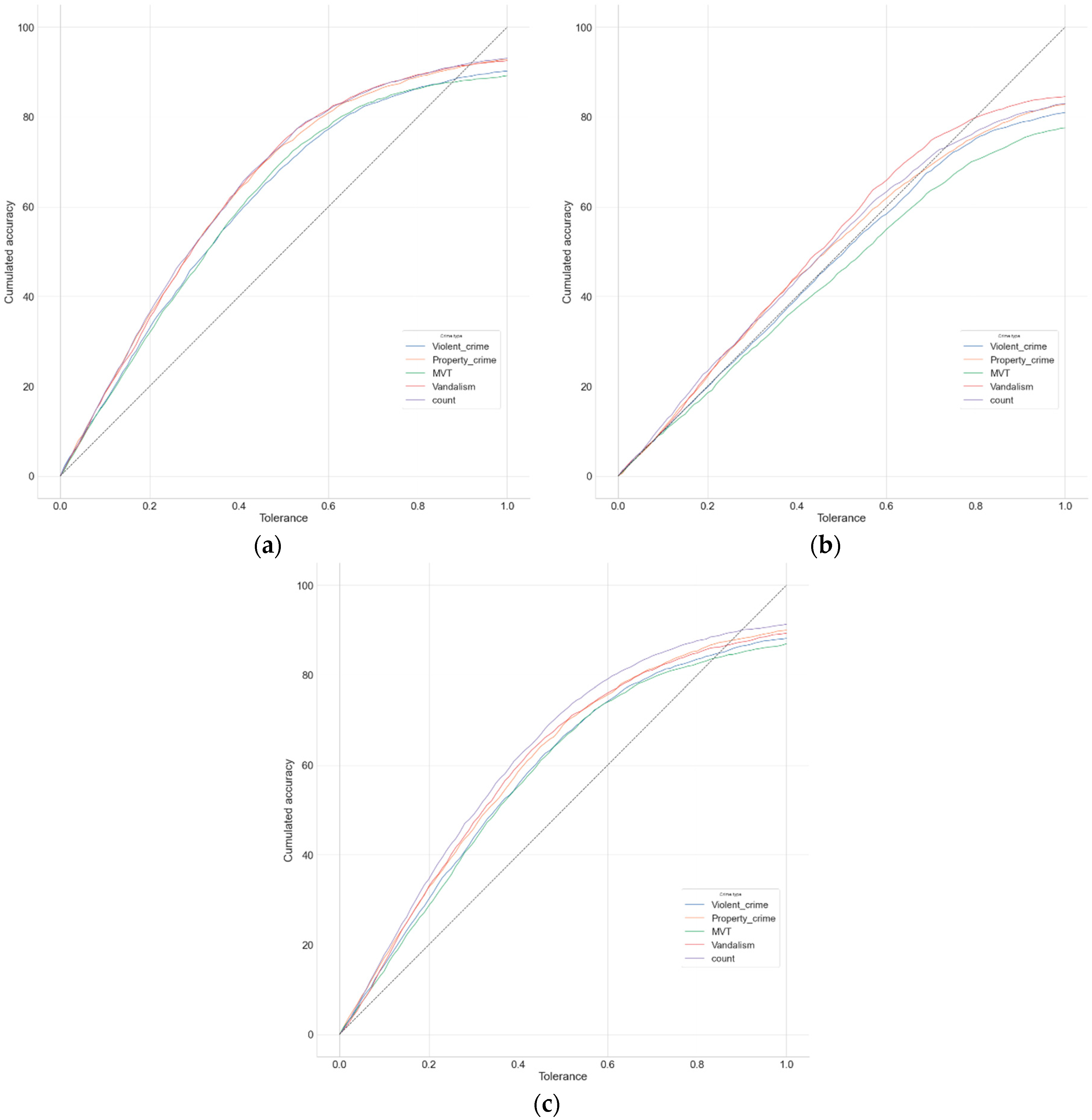
Table 6 shows the performances of three different predictive models, namely Poisson regression, deep learning, and gradient boosting. We applied these models for each crime type, in addition to the total count of crimes, using the same input dataset and in the same conditions. Then, we measured their performance using the MAE and RMSE described above, along with the relative absolute error, the R-squared, and the linear correlation between prediction and observed values. In addition to these results, the regressor error characteristics (REC) curves appear in Figure 2.

Table 6. Comparison of the performance of three predictive models using different evaluation metrics.

Crime Types	Metrics	Models
		Poisson Regression	Deep Learning	Gradient Boosting
Count	MAE	181.94	130.69	123.24
	RMSE	439.35	331.14	318.28
	RAE	102.5%	74.5%	59.7%
	R2	3.6%	45.3%	49.4%
	Pearson Corr.	41.9%	67.7%	71.9%
Violent	MAE	76.41	52.48	49.87
	RMSE	175.70	132.39	132.37
	RAE	118.78%	73.7%	62.4%
	R2	6.1%	46.7%	46.8%
	Pearson Corr.	50.3%	68.6%	70.1%
Property	MAE	114.34	86.61	79.13
	RMSE	309.25	246.30	230.73
	RAE	97.3%	78.3%	56.5%
	R2	1.2%	37.3%	44.3%
	Pearson Corr.	34.2%	62.2%	67.8%
MVT	MAE	15.54	9.35	8.70
	RMSE	37.64	23.28	23.81
	RAE	101.8%	60.3%	51.7%
	R2	1.0%	62.2%	60.5%
	Pearson Corr.	34.2%	79%	80.4%
Vandalism	MAE	28.56	20.18	18.54
	RMSE	56.25	39.04	38.19
	RAE	86.2%	62.9%	51.7%
	R2	2.8%	53.2%	55.3%
	Pearson Corr.	47.6%	73.2%	76.2%

Figure 2. Regression Error Characteristic (REC) curves for (a) the gradient boosting model, (b) the Poisson model, and (c) the deep learning model.

The gradient boosting model outperforms the other models in all the evaluated types of crime and across all metrics. It should be noted, however, that the deep learning model also yields performances close to the gradient boosting results.

In order to further evaluate the performance of these predictive models, we selected a random set of 1000 observations from the input dataset and then we compared the predicted crime occurrences of each type of crime, in addition to the total count of crime occurrences, against the ground truth, as depicted in Figure 3. On this sample of observations, the gradient boosting and the deep learning models yield competitive results compared to the Poisson regression.

Figure 3. Comparison of the predicted occurrences of crimes against the ground truth using three different models. (a) Total crime count: predictions vs. real observations; (b) violent crimes: predictions vs. real observations; (c) property crimes: predictions vs. real observations; (d) MVT: predictions vs. real observations; (e) vandalism: predictions vs. real observations.

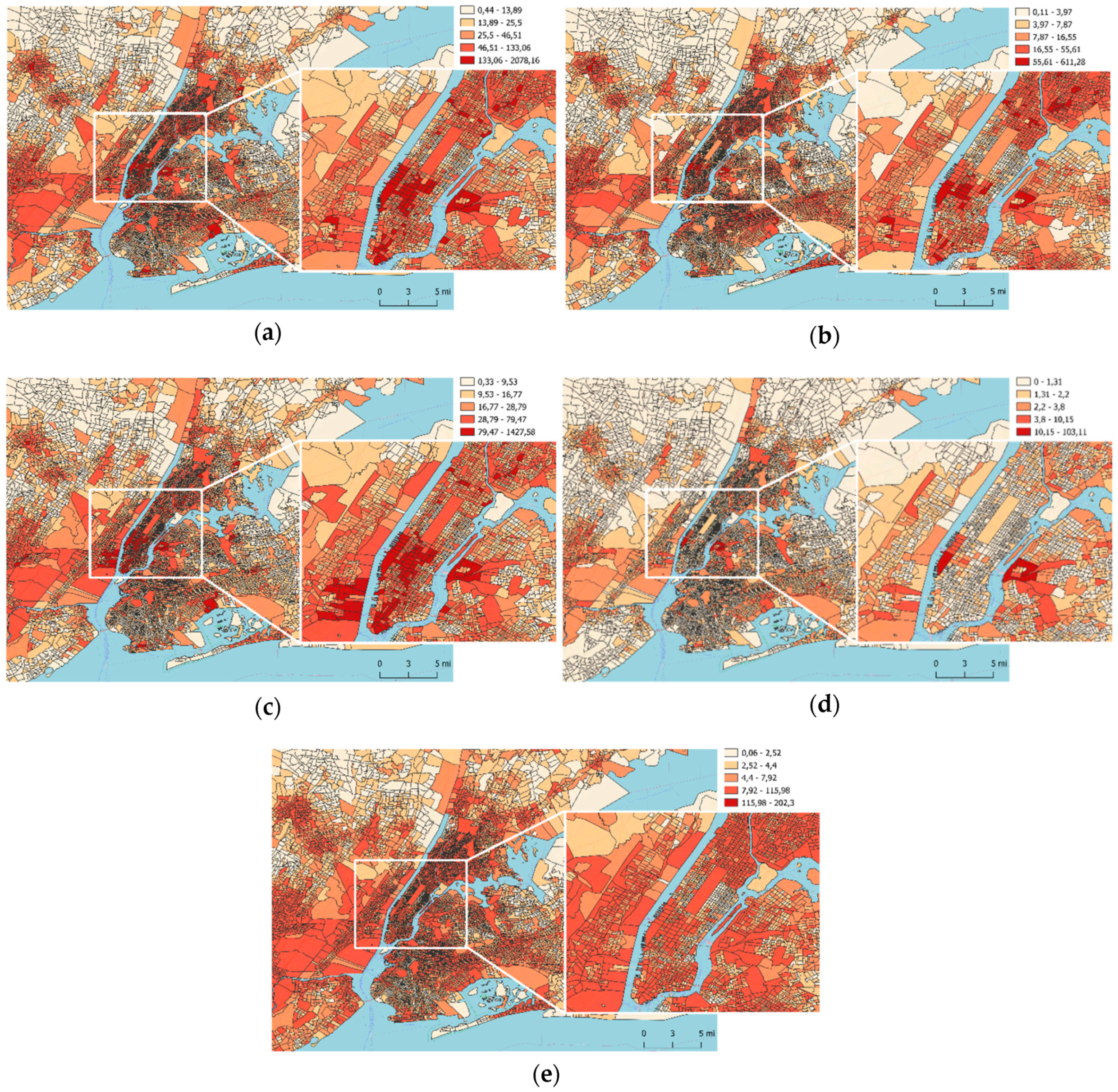
As stated before, our framework is able to provide predicted crime occurrences for all Block Groups in the contiguous U.S. The learning phase was performed on 188 identified features using the split defined p.10, used to predict crime occurrences for 11 U.S. cities across 13,897 Block Groups and for 5 years (2014–2018). The resulting model then generated predictions for crime occurrences for the same period and all U.S. Block Groups. For the sake of clarity, Figure 4 represents our findings for one year using map visualizations of the New York City area, with a focus on Manhattan.

Figure 4. Map visualizations of yearly-predicted crime occurrences in New York City. (a) Predicted total crime (count) occurrences; (b) predicted violent crime occurrences; (c) predicted property crime occurrences; (d) predicted MVT occurrences; (e) predicted vandalism acts. Categories used to generate maps (from light to dark) correspond to the first quartile, second quartile, third quartile, fourth quartile (excluding the 2 highest centiles), and the two highest centiles of crime count predictions, respectively. Basemap obtained from OpenStreetMap, and U.S. Census Block Groups delimitations were extracted from the Tiger Census Shapefiles.

4.4. Discussion

4.4.1. Prediction Results within the Training and Testing Sample

Our approach generates mean absolute errors (MAE) between 36% (vandalism) and 41% (property crime) of the targets’ means, suggesting accuracies between 59% and 64% in our ability to predict the exact count of crimes occurring in a Block Group between 2014 and 2018. This performance can appear moderate in comparison to studies using aggregated data (city, county, state) and past crimes as features that can reach up to 97% accuracy [6]. However, we believe it to be remarkable given that (1) we predict crime at a higher resolution (Census Block Groups) and (2) our approach does not use past crimes as a predictor. Our approach has the advantage of only using features available throughout the entire U.S. Its results can thus provide elements of comparison to policy makers at the national level, including in urban environments where crime data are scarce. Furthermore, our tests reveal that predicting whether an observation lies within one of the categories displayed in Figure 4 instead of the exact crime count can increase our accuracy to 75% when predicting the total count of crimes: 77% for violent crimes, 73% for property crimes, 77% for motor vehicle thefts, and 77% for vandalism acts.

Analyzing the importance of selected features in the decision process can add perspective to our results. The 30 features found to be the most important in our model appear in Table 7.

Table 7. The 30 features with the highest importance, based on the gradient boosting model.

Rank	Feature	Importance (%)
1	Land area	3.61
2	Population density	1.94
3	Total population	1.92
4	Distance to nearest Local Law Enforcement Agency	1.56
5	Number of houses built between 2000–2009 (spillover)	1.26
6	Number of individuals 25+ with an associate’s degree (spillover)	1.15
7	Fraction of people who moved in less than 4 years ago (spillover)	0.99
8	Median Female Age	0.99
9	Median Male Age	0.93
10	% Asian (spillover)	0.88
11	Population 25+ with a master’s degree (spillover)	0.86
12	Total Population with a Bachelor Degree	0.85
13	% Male (spillover)	0.84
14	No vehicle available and householder 35+ (spillover)	0.84
15	Total: some college, less than 1 year: Population 25+ (spillover)	0.84
16	Total: never married	0.84
17	% Black (spillover)	0.83
18	Year structure built: between 2000 and 2009	0.83
19	Ethnic heterogeneity index (spillover)	0.82
20	Single householder, female (spillover)	0.82
21	Fraction of households earning less than USD 10,000/year (spillover)	0.80
22	Number of households earning less than USD 10,000/year (spillover)	0.79
23	Number of individuals in poverty (18+)	0.79
24	% not in labor force (spillover)	0.77
25	Never married (female)	0.77
26	Total: Some college, 1 or more years, no degree: Population 25+	0.77
27	Total: GED or alternative credential: Population 25+	0.76
28	Total: Regular high school diploma: Population 25+ (spillover)	0.76
29	Number of Unemployed individuals	0.75
30	% Other races (spillover)	0.75
	TOTAL:	31.29

The total area covered by the Block Group, which can vary significantly (with larger Block Groups located in rural areas), is the most important predictor (3.6%), followed by population and population density. The median age (aggregating female and male) comes third, followed by the distance to the nearest local law enforcement agency. However, those features collectively explain less than 11% of the total feature importance (with the 10 most important, involving additional factors related to social mobility and education, explaining 17% of the total importance). The diversity of relatively important factors highlights the complexity of crime as a social phenomenon: an important number of features in our framework significantly improve our ability to predict crime occurrences.

Additionally, in many instances, spillover features (i.e., features describing attributes of the neighboring Block Groups) were found as more important than original features (describing attribute of a single Block Group). This is further illustrated by an important spatial autocorrelation in crimes predicted. If we consider total crime throughout the U.S., the Moran’s I (i.e., the correlation between crime in a Block Group and the average crime predicted in neighboring Block Groups) predicted by our approach is around 0.7 nationwide, and the existence of clusters is particularly clear in the case of violent crime, vandalism, and motor vehicle theft (see Figure 4b,d,e for the case of New York).

4.4.2. Prediction Results Outside of the Training and Testing Sample

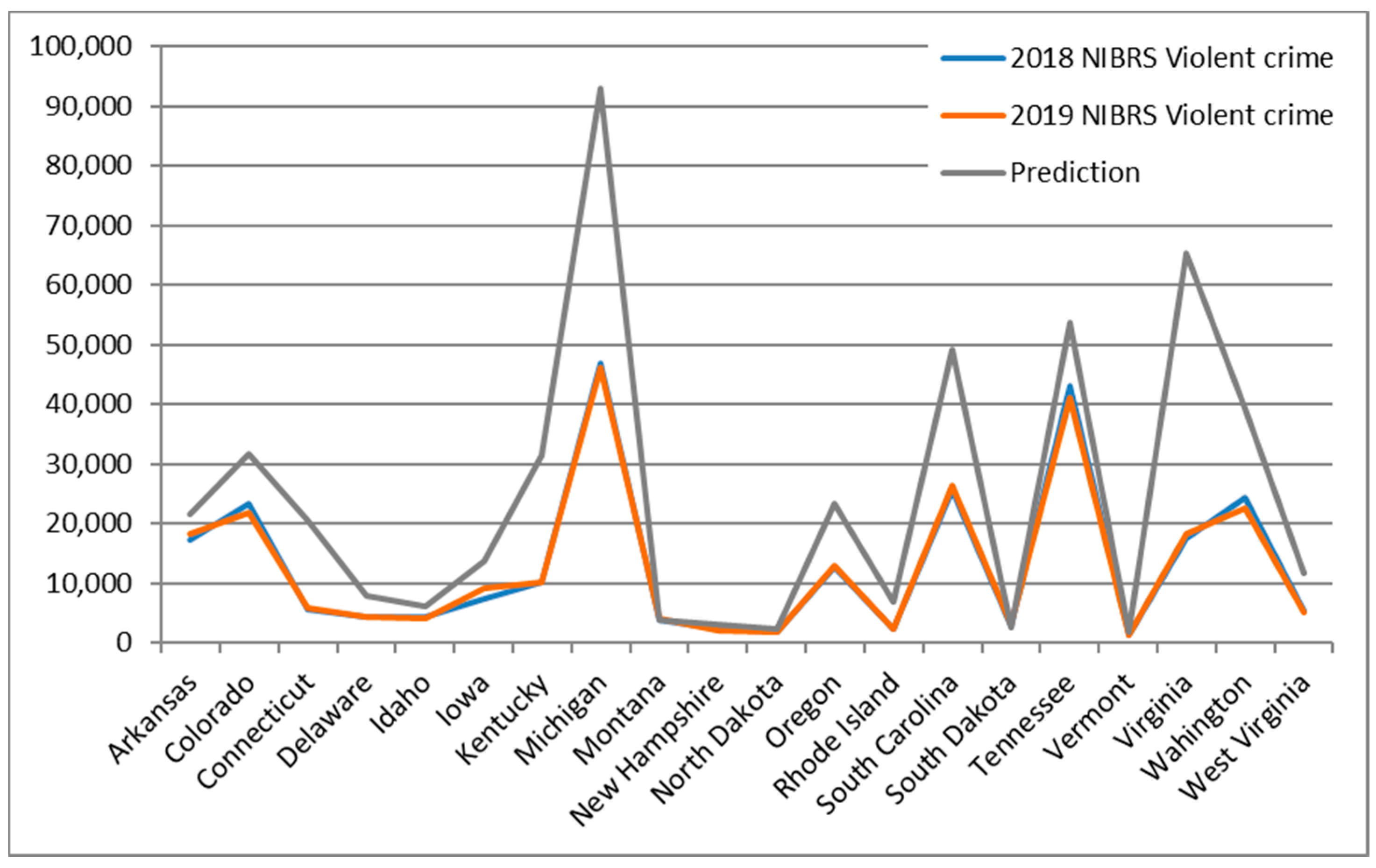
As mentioned in Section 3, our model is trained and tested based on 6.4 % of the total U.S. Block Groups. However, our predictions cover the entire contiguous U.S. Thus, a potential weakness of our model is that the validity of our predictions can be affected by differences between our sample and the total population. In order to provide an additional perspective on our results, aggregated yearly crime predictions at the state level were compared to NIBRS crime data in 17 states where enough data (i.e., where at least 90% of law enforcement agencies reported data to the NIBRS program) were available for 2018 and 2019, using the case of violent crime. Where NIBRS data covered x% of a state’s population, the NIBRS crime count estimate was multiplied by $[1+\left(1-\frac{x}{100}\right)]$. The results appear in Figure 5.

Figure 5. Comparison of the predicted crime occurrences against the NIBRS data at the state level.

At the aggregated state level, the comparison between our predictions and NIBRS data in 2019 reveals a correlation of 90.8%. Overall, the R2 of the linear regression of NIBRS data on predictions is 82.4%, suggesting that our predictions reflect the trends observed in crime data across states where it can be observed.

However, in the case of violent crime, a general trend towards crime overestimation can be noted in absolute terms. In states such as Virginia, Connecticut, and Kentucky, the overestimation is particularly high and can limit our model’s usability. These states tend to display under-average crime rates as defined by the NIBRS program (204.2, 209.6 and 217.9 crimes per 100k inhabitants, against a 383.4 U.S. average).

In contrast, predictions are close to the NIBRS data in states such as South Dakota and Montana, where the gaps between predictions and NIBRS totals represent −2% and 1% of NIBRS totals, respectively. Note that these comparisons should be analyzed with caution, due to the difference in data sources involved: our sample is based on the Open Crime Database, gathering incident data from various city-level geodatabases [11], while NIBRS data are based on the FBI Uniform Crime Report program.

Finally, if we consider each state’s rank position in terms of crime count, our model shows a satisfactory performance: the rank-order correlation between prediction and 2018 NIBRS data is 95.8%, and the maximal error is four ranks (i.e., Rhode Island is predicted to rank 14th, but found to rank 18th in the NIBRS data; Virginia is predicted to be 2nd, and found 6th among the 20 states considered). Our model successfully predicts whether a state is in the 1st, 2nd, 3rd, or 4th quartile in terms of aggregated violent crime among the 20 states considered in 60% of cases.

Overall, comparisons between model predictions and 2018 NIBRS data at the state aggregated level suggest that our model generates predictions involving significant overestimations in absolute terms (crime count predictions), but reproduces crime trends across states (as displayed by correlation and R-squared) and shows a reasonable performance in predicting a state’s rank in terms of violent crimes.

4.4.3. Limitations

Finally, a number of limitations should be stated. First, due to the methodological framework used, we can identify features of importance but not their impact (positive or negative) on crime in our model. Second, our approach is based on more than 180 features gathered from multiple different sources. Therefore, it involves a significant amount of work in terms of data processing. Third, our accuracy could be improved by adding additional types of features to the analysis. These could include point of interests (involving a significant amount of social interaction), such as bus stops [2], malls, bars, churches, or schools [79], factors related to street lights [76] and/or social networks data [90] to complement our analysis and potentially mitigate the overestimations identified in some states. Considering ambient population instead of residential population [91] is also a promising perspective for future research. In some states, Section 4.4.2 identified significant overestimations in the crime counts predicted, in spite of a reasonable relative performance. Finally, our model is trained on various urban contexts, meaning that it does not necessarily capture crime dynamics in rural settings. Consequently, predictions relative to rural areas might be more uncertain than their urban counterparts.

5. Conclusions

In this paper, we proposed an ML framework able to provide predictions for spatial crime occurrences across all U.S. Census Block Groups in the contiguous U.S. Our findings from a set of extensive experiments on real-world datasets of crimes reported in 11 U.S. cities demonstrate that the proposed framework yields accurate predictions for the different crime types considered—i.e., violent crimes, property crimes, motor vehicle thefts, vandalism acts, and total count of crime occurrences. For these crime types, our ability to predict whether crime count in a Block Group belongs to the first, second, third, or fourth quartile or the two highest centiles range between 73% and 77%. Comparing model predictions and NIBRS crime data outside of the sample used to train and test the model suggests significant a trend towards overestimations in absolute crime count predictions, particularly marked for specific states, including Virginia and Kentucky. However, the model shows a satisfactory performance in relative terms, as measured by the rank-order correlation between states predictions and NIBRS and quartile analysis.

We believe that our findings (and in particular the mentioned overestimations) could be further enhanced by considering additional features, such as social networks data, sites involving significant amounts of social interaction (malls, bars, churches, schools, etc.), land use, and streetlights. Another path to explore deeply in future research could be the subject of rural crime. Although many factors defining rural areas (such as lower population density) have indeed been taken into account by our model, differing societal frameworks might justify the use of a separate model in the future.

References

1. Clancey, G. Are We Still ‘Flying Blind?’ Crime Data and Local Crime Prevention in New South Wales. Curr. Issues Crim. Justice 2011, 22, 491–500. [Google Scholar] [CrossRef]
2. Cichosz, P. Urban Crime Risk Prediction Using Point of Interest Data. ISPRS Int. J. Geo-Inf. 2020, 9, 459. [Google Scholar] [CrossRef]
3. Inayatullah, S. The Futures of Policing: Going beyond the Thin Blue Line. Futures 2013, 49, 1–8. [Google Scholar] [CrossRef]
4. Almaw, A.; Kadam, K. Survey Paper on Crime Prediction Using Ensemble Approach. Int. J. Pure Appl. Math. 2018, 118, 133–139. [Google Scholar]
5. Prabakaran, S.; Mitra, S. Survey of Analysis of Crime Detection Techniques Using Data Mining and Machine Learning. J. Phys. Conf. Ser. 2018, 1000, 012046. [Google Scholar] [CrossRef]
6. Alves, L.G.A.; Ribeiro, H.V.; Rodrigues, F.A. Crime Prediction through Urban Metrics and Statistical Learning. Phys. A Stat. Mech. Its Appl. 2018, 505, 435–443. [Google Scholar] [CrossRef]
7. Kadar, C.; Maculan, R.; Feuerriegel, S. Public Decision Support for Low Population Density Areas: An Imbalance-Aware Hyper-Ensemble for Spatio-Temporal Crime Prediction. Decis. Support Syst. 2019, 119, 107–117. [Google Scholar] [CrossRef]
8. Lin, Y.-L.; Yen, M.-F.; Yu, L.-C. Grid-Based Crime Prediction Using Geographical Features. ISPRS Int. J. Geo-Inf. 2018, 7, 298. [Google Scholar] [CrossRef]
9. Meijer, A.; Wessels, M. Predictive Policing: Review of Benefits and Drawbacks. Int. J. Public Adm. 2019, 42, 1031–1039. [Google Scholar] [CrossRef]
10. Konkel, R.H.; Ratkowski, D.; Tapp, S.N. The Effects of Physical, Social, and Housing Disorder on Neighborhood Crime: A Contemporary Test of Broken Windows Theory. ISPRS Int. J. Geo-Inf. 2019, 8, 583. [Google Scholar] [CrossRef]
11. Ashby, M.P.J. Studying Crime and Place with the Crime Open Database: Social and Behavioural Scienes. Res. Data J. Humanit. Soc. Sci. 2018. [Google Scholar] [CrossRef]
12. Shaw, C.R.; McKay, H.D. Juvenile Delinquency and Urban Areas; University of Chicago Press: Chicago, IL, USA, 1942. [Google Scholar]
13. Pratt, T.C.; Cullen, F.T. Assessing Macro-Level Predictors and Theories of Crime: A Meta-Analysis. Crime Justice 2005, 32, 373–450. [Google Scholar] [CrossRef]
14. Bursik, R.J. Social Disorganization and Theories of Crime and Delinquency: Problems and Prospects. Criminology 1988, 26, 519–552. [Google Scholar] [CrossRef]
15. Kornhauser, R.R. Social Sources of Delinquency: An Appraisal of Analytic Models; University of Chicago Press: Chicago, IL, USA, 1978. [Google Scholar]
16. Sampson, R.; Groves, W.B. Community Structure and Crime: Testing Social-Disorganization Theory. Am. J. Sociol. 1989. [Google Scholar] [CrossRef]
17. Bursik, R.J.J.; Grasmick, H.G. Economic Deprivation and Neighborhood Crime Rates 1960–1980. Law Soc. Rev. 1993, 27, 263. [Google Scholar]
18. Sampson, R.J.; Raudenbush, S.W.; Earls, F. Neighborhoods and Violent Crime: A Multilevel Study of Collective Efficacy. Science 1997, 277, 918–924. [Google Scholar] [CrossRef] [PubMed]
19. Wilson, W.J. The Truly Disadvantaged: The Inner City, the Underclass, and Public Policy; University of Chicago Press: Chicago, IL, USA, 1987. [Google Scholar]
20. Cole, S.J. Social and Physical Neighbourhood Effects and Crime: Bringing Domains Together Through Collective Efficacy Theory. Soc. Sci. 2019, 8, 147. [Google Scholar] [CrossRef]
21. Browning, C.R. The Span of Collective Efficacy: Extending Social Disorganization Theory to Partner Violence. J. Marriage Fam. 2002, 64, 833–850. [Google Scholar] [CrossRef]
22. Morenoff, J.D.; Sampson, R.J.; Raudenbush, S.W. Neighborhood Inequality, Collective Efficacy, and the Spatial Dynamics of Urban Violence. Criminology 2001, 39, 517–558. [Google Scholar] [CrossRef]
23. Sampson, R.J.; Wikström, P.-O.H. The Social Order of Violence in Chicago and Stockholm Neighborhoods: A Comparative Inquiry. In Order, Conflict, and Violence; Shapiro, I., Kalyvas, S.N., Masoud, T., Eds.; Cambridge University Press: Cambridge, UK, 2008; pp. 97–119. [Google Scholar] [CrossRef]
24. Cohen, L.E.; Felson, M. Social Change and Crime Rate Trends: A Routine Activity Approach. Am. Sociol. Rev. 1979, 44, 588–608. [Google Scholar] [CrossRef]
25. Weisburd, D.; Groff, E.R.; Yang, S.-M. The Criminology of Place: Street Segments and Our Understanding of the Crime Problem; Oxford University Press: Oxford, UK, 2012. [Google Scholar]
26. Spano, R.; Freilich, J.D. An Assessment of the Empirical Validity and Conceptualization of Individual Level Multivariate Studies of Lifestyle/Routine Activities Theory Published from 1995 to 2005. J. Crim. Justice 2009, 37, 305–314. [Google Scholar] [CrossRef]
27. Andresen, M.A. A Spatial Analysis of Crime in Vancouver, British Columbia: A Synthesis of Social Disorganization and Routine Activity Theory. Can. Geogr./Le Géographe Can. 2006, 50, 487–502. [Google Scholar] [CrossRef]
28. Furstenberg, F.F.; Cook, T.D.; Eccles, J.; Elder, G.H.; Sameroff, A. Managing To Make It: Urban Families and Adolescent Success. Studies on Successful Adolescent Development; University of Chicago Press: Chicago, IL, USA, 2000. [Google Scholar]
29. Brisson, D.; Roll, S. The Effect of Neighborhood on Crime and Safety: A Review of the Evidence. Null 2012, 9, 333–350. [Google Scholar] [CrossRef] [PubMed]
30. Coleman, J.S. Social Capital in the Creation of Human Capital. Am. J. Sociol. 1988, 94, S95–S120. [Google Scholar] [CrossRef]
31. Putnam, R.D. Bowling Alone: The Collapse and Revival of American Community. In Bowling Alone: The Collapse and Revival of American Community; Touchstone Books/Simon & Schuster: New York, NY, USA, 2000; p. 541. [Google Scholar] [CrossRef]
32. Chiu, W.H.; Madden, P. Burglary and Income Inequality. J. Public Econ. 1998, 69, 123–141. [Google Scholar] [CrossRef]
33. Hsieh, C.-C.; Pugh, M.D. Poverty, Income Inequality, and Violent Crime: A Meta-Analysis of Recent Aggregate Data Studies. Crim. Justice Rev. 1993, 18, 182–202. [Google Scholar] [CrossRef]
34. Kelly, M. Inequality and Crime. Rev. Econ. Stat. 2000, 82, 530–539. [Google Scholar] [CrossRef]
35. Weatherburn, D. What Causes Crime? NSW Bureau of Crime Statistics and Research: Sydney, Australia, 2001.
36. Feldmeyer, B. The Effects of Racial/Ethnic Segregation on Latino and Black Homicide. Sociol. Q. 2010, 51, 600–623. [Google Scholar] [CrossRef]
37. Krivo, L.J.; Peterson, R.D.; Kuhl, D.C. Segregation, Racial Structure, and Neighborhood Violent Crime. Am. J. Sociol. 2009, 114, 1765–1802. [Google Scholar] [CrossRef]
38. Peterson, R.D.; Krivo, L.J. Divergent Social Worlds: Neighborhood Crime and the Racial-Spatial Divide; Russell Sage Foundation: New York, NY, USA, 2010. [Google Scholar]
39. Balkwell, J.W. Ethnic Inequality and the Rate of Homicide. Soc. Forces 1990, 69, 53–70. [Google Scholar] [CrossRef]
40. Blau, P.M.; Golden, R.M. Metropolitan Structure and Criminal Violence. Sociol. Q. 1986, 27, 15–26. [Google Scholar] [CrossRef]
41. Kubrin, C. Racial Heterogeneity and Crime: Measuring Static and Dynamic Effects. Res. Community Sociol. 2000, 10, 189–219. [Google Scholar]
42. Warner, B.D.; Rountree, P.W. Local Social Ties in a Community and Crime Model: Questioning the Systemic Nature of Informal Social Control. Soc. Probl. 1997, 44, 520–536. [Google Scholar] [CrossRef]
43. Schieman, S. Residential Stability and the Social Impact of Neighborhood Disadvantage: A Study of Gender-and Race-Contingent Effects. Soc. Forces 2005, 83, 1031–1064. [Google Scholar] [CrossRef]
44. Burton, V.S., Jr.; Cullen, F.T.; Evans, T.D.; Alarid, L.F.; Dunaway, R.G. Gender, Self-Control, and Crime. J. Res. Crime Delinq. 1998, 35, 123–147. [Google Scholar] [CrossRef]
45. Carrabine, E.; Iganski, P.; South, N.; Lee, M.; Plummer, K.; Turton, J.; Iganski, P.; South, N.; Lee, M.; Plummer, K.; et al. Criminology: A Sociological Introduction; Routledge: Arbington, UK, 2004. [Google Scholar] [CrossRef]
46. Chrisler, J.C.; McCreary, D.R. Handbook of Gender Research in Psychology; Springer: Berlin/Heidelberg, Germany, 2010; Volume 1. [Google Scholar]
47. Rowe, D.C.; Vazsonyi, A.T.; Flannery, D.J. Sex Differences in Crime: Do Means and within-Sex Variation Have Similar Causes? J. Res. Crime Delinq. 1995, 32, 84–100. [Google Scholar] [CrossRef]
48. Hirschi, T.; Gottfredson, M. Age and the Explanation of Crime. Am. J. Sociol. 1983, 89, 552–584. [Google Scholar] [CrossRef]
49. Farrington, D.P. Childhood Aggression and Adult Violence: Early Precursors and Later-Life Outcomes. Dev. Treat. Child. Aggress. 1991, 5, 29. [Google Scholar]
50. Flanagan, T.J.; Maguire, K. Sourcebook of Criminal Justice Statistics—1989; Department of Justice, Bureau of Justice Statistics: Washington, DC, USA, 1990.
51. Sampson, R.J.; Morenoff, J.D.; Gannon-Rowley, T. Assessing “Neighborhood Effects”: Social Processes and New Directions in Research. Annu. Rev. Sociol. 2002, 28, 443–478. [Google Scholar] [CrossRef]
52. Land, K.C.; McCall, P.L.; Cohen, L.E. Structural Covariates of Homicide Rates: Are There Any Invariances across Time and Social Space? Am. J. Sociol. 1990, 95, 922–963. [Google Scholar] [CrossRef]
53. Messner, S.F.; Rosenfeld, R.; Baumer, E.P. Dimensions of Social Capital and Rates of Criminal Homicide. Am. Sociol. Rev. 2004, 69, 882–903. [Google Scholar] [CrossRef]
54. Lo, C.C.; Zhong, H. Linking Crime Rates to Relationship Factors: The Use of Gender-Specific Data. J. Crim. Justice 2006, 34, 317–329. [Google Scholar] [CrossRef]
55. Sharkey, P.T. Navigating Dangerous Streets: The Sources and Consequences of Street Efficacy. Am. Sociol. Rev. 2006, 71, 826–846. [Google Scholar] [CrossRef]
56. McLanahan, S.; Bumpass, L. Intergenerational Consequences of Family Disruption. Am. J. Sociol. 1988, 94, 130–152. [Google Scholar] [CrossRef]
57. Messner, S.F.; Sampson, R.J. The Sex Ratio, Family Disruption, and Rates of Violent Crime: The Paradox of Demographic Structure. Soc. Forces 1991, 69, 693–713. [Google Scholar] [CrossRef]
58. Sampson, R.J. Neighborhood Family Structure and the Risk of Personal Victimization. In The Social Ecology of Crime; Springer: Berlin/Heidelberg, Germany, 1986; pp. 25–46. [Google Scholar]
59. Lyons, C.J. Community (Dis) Organization and Racially Motivated Crime. Am. J. Sociol. 2007, 113, 815–863. [Google Scholar] [CrossRef]
60. Frye, V. The Informal Social Control of Intimate Partner Violence against Women: Exploring Personal Attitudes and Perceived Neighborhood Social Cohesion. J. Community Psychol. 2007, 35, 1001–1018. [Google Scholar] [CrossRef]
61. Cantillon, D. Community Social Organization, Parents, and Peers as Mediators of Perceived Neighborhood Block Characteristics on Delinquent and Prosocial Activities. Am. J. Community Psychol. 2006, 37, 111–127. [Google Scholar] [CrossRef]
62. Bellair, P.E. Social Interaction and Community Crime: Examining the Importance of Neighbor Networks. Criminology 1997, 35, 677–704. [Google Scholar] [CrossRef]
63. Browning, C.R.; Dietz, R.D.; Feinberg, S.L. The Paradox of Social Organization: Networks, Collective Efficacy, and Violent Crime in Urban Neighborhoods. Soc. Forces 2004, 83, 503–534. [Google Scholar] [CrossRef]
64. Gibson, C.L.; Zhao, J.; Lovrich, N.P.; Gaffney, M.J. Social Integration, Individual Perceptions of Collective Efficacy, and Fear of Crime in Three Cities. Justice Q. 2002, 19, 537–564. [Google Scholar] [CrossRef]
65. Wells, L.E.; Weisheit, R.A. Patterns of Rural and Urban Crime: A County-Level Comparison. Crim. Justice Rev. 2004, 29, 1–22. [Google Scholar] [CrossRef]
66. Kaylen, M.T.; Pridemore, W.A. Social Disorganization and Crime in Rural Communities: The First Direct Test of the Systemic Model. Br. J. Criminol. 2013, 53, 905–923. [Google Scholar] [CrossRef]
67. Bouffard, L.A.; Muftić, L.R. The “Rural Mystique”: Social Disorganization and Violence beyond Urban Communities. West. Criminol. Rev. 2006, 7, 56–66. [Google Scholar]
68. Li, Y.-Y. Social Structure and Informal Social Control in Rural Communities. Int. J. Rural Criminol. 2011, 1, 63–88. [Google Scholar] [CrossRef]
69. Petee, T.A.; Kowalski, G.S. Modeling Rural Violent Crime Rates: A Test of Social Disorganization Theory. Sociol. Focus 1993, 26, 87–89. [Google Scholar] [CrossRef]
70. Osgood, D.W.; Chambers, J.M. Social Disorganization Outside the Metropolis: An Analysis of Rural Youth Violence. Criminology 2000, 38, 81–116. [Google Scholar] [CrossRef]
71. Wells, L.E.; Weisheit, R.A. Explaining Crime in Metropolitan and Non-Metropolitan Communities. Int. J. Rural Criminol. 2013, 1, 153–183. [Google Scholar] [CrossRef][Green Version]
72. Barnett, C.; Mencken, F.C. Social Disorganization Theory and the Contextual Nature of Crime in Nonmetropolitan Counties. Rural Sociol. 2002, 67, 372–393. [Google Scholar] [CrossRef]
73. Osgood, D.W.; Chambers, J.M. Community Correlates of Rural Youth Violence. Juv. Justice Bull. 2003, 1–12. Available online: https://www.ncjrs.gov/pdffiles1/ojjdp/193591.pdf (accessed on 29 October 2020).
74. Ward, K.C.; Kirchner, E.E.; Thompson, A.J. Social Disorganization and Rural/Urban Crime Rates: A County Level Comparison of Contributing Factors. Int. J. Rural. Criminol. 2018, 4, 43–65. [Google Scholar] [CrossRef]
75. Kaylen, M.; Pridemore, W.A.; Roche, S.P. The Impact of Changing Demographic Composition on Aggravated Assault Victimization during the Great American Crime Decline: A Counterfactual Analysis of Rates in Urban, Suburban, and Rural Areas. Crim. Justice Rev. 2017, 42, 291–314. [Google Scholar] [CrossRef]
76. Kang, H.-W.; Kang, H.-B. Prediction of Crime Occurrence from Multi-Modal Data Using Deep Learning. PLoS ONE 2017, 12, e0176244. [Google Scholar] [CrossRef] [PubMed]
77. Huang, C.; Zhang, J.; Zheng, Y.; Chawla, N.V. DeepCrime: Attentive Hierarchical Recurrent Networks for Crime Prediction. In Proceedings of the 27th ACM International Conference on Information and Knowledge Management, CIKM ’18; Association for Computing Machinery: Torino, Italy, 2018; pp. 1423–1432. [Google Scholar] [CrossRef]
78. Marchant, R.; Haan, S.; Clancey, G.; Cripps, S. Applying Machine Learning to Criminology: Semi-Parametric Spatial-Demographic Bayesian Regression. Secur. Inform. 2018, 7, 1. [Google Scholar] [CrossRef]
79. Ingilevich, V.; Ivanov, S. Crime Rate Prediction in the Urban Environment Using Social Factors. Procedia Comput. Sci. 2018, 136, 472–478. [Google Scholar] [CrossRef]
80. US Census Bureau. 2014–2018 ACS 5-year Estimates. Available online: https://www.census.gov/programs-surveys/acs/technical-documentation/table-and-geography-changes/2018/5-year.html (accessed on 18 August 2020).
81. Fick, S.E.; Hijmans, R.J. WorldClim 2: New 1-Km Spatial Resolution Climate Surfaces for Global Land Areas. Int. J. Climatol. 2017, 37, 4302–4315. [Google Scholar] [CrossRef]
82. Breiman, L.; Friedman, J.; Stone, C.J.; Olshen, R.A. Classification and Regression Trees; Routledge & CRC Press: Abingdon, UK, 1984. [Google Scholar]
83. Pedregosa, F.; Varoquaux, G.; Gramfort, A.; Michel, V.; Thirion, B.; Grisel, O.; Blondel, M.; Prettenhofer, P.; Weiss, R.; Dubourg, V.; et al. Scikit-Learn: Machine Learning in Python. J. Mach. Learn. Res. 2011, 12, 2825–2830. [Google Scholar]
84. Virtanen, P.; Gommers, R.; Oliphant, T.E.; Haberland, M.; Reddy, T.; Cournapeau, D.; Burovski, E.; Peterson, P.; Weckesser, W.; Bright, J.; et al. SciPy 1.0--Fundamental Algorithms for Scientific Computing in Python. Nat. Methods 2020, 17, 261–272. [Google Scholar] [CrossRef]
85. Armitage, R.; Monchuk, L.; Rogerson, M. It Looks Good, but What Is It like to Live There? Exploring the Impact of Innovative Housing Design on Crime. Eur. J. Crim. Policy Res. 2011, 17, 29–54. [Google Scholar] [CrossRef]
86. Mouatassim, Y.; Ezzahid, E.H. Poisson Regression and Zero-Inflated Poisson Regression: Application to Private Health Insurance Data. Eur. Actuar. J. 2012, 2, 187–204. [Google Scholar] [CrossRef]
87. Fallah, N.; Gu, H.; Mohammad, K.; Seyyedsalehi, S.A.; Nourijelyani, K.; Eshraghian, M.R. Nonlinear Poisson Regression Using Neural Networks: A Simulation Study. Neural Comput. Appl. 2009, 18, 939. [Google Scholar] [CrossRef]
88. Friedman, J.H. Greedy Function Approximation: A Gradient Boosting Machine. Ann. Stat. 2001, 29, 1189–1232. [Google Scholar] [CrossRef]
89. Zhang, Z. Parameter Estimation Techniques: A Tutorial with Application to Conic Fitting; Research Report RR-2676; INRIA: Sophia Antipolis, France, 1995; pp. 59–76. [Google Scholar]
90. Bogomolov, A.; Lepri, B.; Staiano, J.; Oliver, N.; Pianesi, F.; Pentland, A. Once Upon a Crime: Towards Crime Prediction from Demographics and Mobile Data. In Proceedings of the 16th International Conference on Multimodal Interaction, ICMI ’14, Istanbul, Turkey, 12–16 November 2014; Association for Computing Machinery: New York, NY, USA, 2014; pp. 427–434. [Google Scholar] [CrossRef]
91. He, L.; Páez, A.; Jiao, J.; An, P.; Lu, C.; Mao, W.; Long, D. Ambient Population and Larceny-Theft: A Spatial Analysis Using Mobile Phone Data. Isprs Int. J. Geo-Inf. 2020, 9, 342. [Google Scholar] [CrossRef]
Publisher’s Note: MDPI stays neutral with regard to jurisdictional claims in published maps and institutional affiliations.
Article Metrics
Citations
Article Access Statistics
Multiple requests from the same IP address are counted as one view.