Article

Retrieval of Leaf Area Index Using Sentinel-2 Imagery in a Mixed Mediterranean Forest Area

by
Irene Chrysafis
1,
Georgios Korakis
1,
Apostolos P. Kyriazopoulos
1 and
Giorgos Mallinis
2,*
1
Department of Forestry and Management of the Environment and Natural Resources, Democritus University of Thrace, GR 68200 Orestiada, Greece
2
School of Rural and Surveying Engineering, Aristotle University of Thessaloniki, GR 54124 Thessaloniki, Greece
*
Author to whom correspondence should be addressed.
ISPRS Int. J. Geo-Inf. 2020, 9(11), 622; https://doi.org/10.3390/ijgi9110622
Submission received: 18 September 2020 / Revised: 7 October 2020 / Accepted: 22 October 2020 / Published: 24 October 2020

Abstract

:
Leaf area index (LAI) is a crucial biophysical indicator for assessing and monitoring the structure and functions of forest ecosystems. Improvements in remote sensing instrumental characteristics and the availability of more efficient statistical algorithms, elevate the potential for more accurate models of vegetation biophysical properties including LAI. The aim of this study was to assess the spectral information of Sentinel-2 MSI satellite imagery for the retrieval of LAI over a mixed forest ecosystem located in northwest Greece. Forty-eight field plots were visited for the collection of ground LAI measurements using an ACCUPAR LP-80: PAR & LAI Ceptometer. Spectral bands and spectral indices were used for LAI model development using the Gaussian processes regression (GPR) algorithm. A variable selection procedure was applied to improve the model’s prediction accuracy, and variable importance was investigated for identifying the most informative variables. The model resulting from spectral indices’ variables selection produced the most precise predictions of LAI with a coefficient of determination of 0.854. Shortwave infrared bands and the normalized canopy index (NCI) were identified as the most important features for LAI prediction.

Graphical Abstract

1. Introduction

Leaf area index (LAI), commonly defined as the amount of leaf area (m2) in a canopy per unit of ground area (m2) [1,2], is a critical biophysical indicator recognized as an essential climate variable (ECV). LAI is applicable in evaluating land ecosystem condition and functions, as well as observing various characteristics of global ecosystems [3]. It can also be applied for the evaluation of the photosynthetic capacity of vegetation as a function of available leaf area [4]. The total amount of leaf area is an important vegetation parameter that can be used to model and quantify the role of vegetation cover to many Earth’s surface processes, such as primary productivity, rainfall interception, and carbon flux [5]. Thus, LAI can be used as a tool for adapting and implementing more sustainable forest management practices [6].
Direct field measurements such as point contact sampling, litterfall traps, or destructive sampling (area harvest) are considered to be the most accurate approach to estimate LAI. However, these processes are labor-intensive and are often constrained by site accessibility, logistical, staff-related and financial factors [7]. Improved indirect, non-destructive field-based techniques such as the indirect point quadrat, allometric and canopy gap fraction analysis through terrestrial sensors, and have an increased cost-efficiency of the traditional in situ approach. However, ground measurements cannot provide LAI information over large areas and extended temporal periods [8].
At the present time, airborne and satellite, passive and active sensors are used for the rapid, spatial explicit retrieval of LAI [9]. Satellite sensors assist the potential to retrieve LAI values from local to global scales, relying on the specific spectral attributes of green leaves (i.e., strong absorption in the visible and high reflectance in the near infrared) compared with other land surface materials [5].
Currently, LAI estimating methods based on optical remote sensing include the development of empirical relationships between LAI and spectral/spatial information, biophysical modeling (inversion of radiative transfer models simulating canopy reflectance), and hybrid inversion methods [10,11]. Empirical approaches (parametric or non-parametric models) are set up on the association between texture or spectral features and field LAI values defined over sample plots. In the second approach (i.e., biophysical modeling), LAI is estimated through a reverse physical model using spectral reflectance as the input variable and LAI as the model’s output. Finally, the hybrid inversion approach integrates statistical and physical models [12,13]. Compared to the statistical models, the last two approaches are considered more accurate, generalizing well across a wider area extent, however, they are more time and data demanding during the training phase [14,15].
The most common approach for LAI estimation through remote sensing data relies upon the use of spectral vegetation indices, and it is a relatively simple and computationally efficient approach [11,15,16]. Vegetation indices serving as proxy indicators of the vegetation’s surface reflectance which can be used in order to reduce the dimensionality and redundancy of spectral information, as well as confounding variables such as scene illumination, soil background, topography or atmospheric effects [5,17]. Nevertheless, the statistical relationships between remotely sensed LAI and spectral indices are ecosystem dependent and do not typically generalize well across different ecosystems [16,18].
Until recently, Landsat imagery was the most frequent source of information for LAI, due to its spatial resolution, large area coverage, and free availability from the end of 2008 [11]. The launch of Sentinel-2A on 2015, providing a high revisit time and a spatial resolution imagery up to 10 m, also at no-cost, increased the analysis accuracy of biophysical parameters such as LAI which has been anticipated due its higher spatial/spectral resolution and higher revisit frequency [4]. In particular, Sentinel-2, apart from six bands that are comparable to Landsat-8, offers three bands in the red-edge part of the spectrum, met at 705, 740 and 783 nm. These additional bands located in the sharp-edge between the red absorption maximum and the near-infrared reflectance, respond to canopy reflectance as resulting from the multiple scattering among leaf layers [5,15]. In addition, spectral information from the red-edge region of the spectrum is less affected by biophysical attributes such as canopy structure and leaf spectral properties, solar zenith angle irradiance, and other atmospheric effects [19]. However, the improvement of LAI retrieval through the exploitation of spectral information available in the red-edge position of the reflectance spectrum is still open to research, since several studies presented controversy results [5,15].
Along with the advances in sensor characteristics, new approaches have been introduced for statistical model development, providing a more robust framework to model complex dynamics. The majority of the studies developing LAI prediction models over forest environments rely on the use of simple and multiple regression-based (i.e., linear, log-linear or exponential) models [5,11]. However, conventional regression methods might be insufficient for multiple independent predictors, such as multiple vegetation indices [12], because of its weakness to handle high-dimensional nonlinear relationships, multi-collinearity limitations, and normal distribution requirement [20], raising the need for enhanced modeling approaches.
Statistical machine learning methods including nonlinear and linear, non-parametric models such as support vector regression (SVR) [20,21,22], neural networks (NN) [20,23,24], partial least squares regression (PLSR) [23,25], random forest (RF) [22,26,27], and Gaussian process regression (GPR) [27,28,29] are modeling alternatives that have been applied to build predictive models of LAI [30] with high-dimensional characteristic parameters [12].
Meyer et al. [5] developed simple and multiple linear regression models for LAI estimation in a temperate forest in the southeastern Germany, using Landsat-8 and Sentinel-2 data. Omner et al. [20] compared SVM and NN regression models for the LAI retrieval of endangered tree species in South Africa, using WorldView imagery. SVM regression was also employed by Durbha et al. [21] to estimate LAI from multiangle imaging spectroradiometer in an agricultural area in France. Wang et al. [22] estimated the LAI of grassland in Oklahoma, United States, using Sentinel-1, Sentinel-2, and Landsat data in SVM and RF models. Cohrs et al. [16] used SVM classification to enhance the linear models of LAI-2200C data and the spectral information of Sentinel-2, in a pine plantation. Kial et al. [25] employed the PLSR algorithm to predict LAI in a grassland area, using hyperspectral data. Houborg et al. [26] assessed LAI in an agricultural area, suggesting a hybrid model on the base of decision tree regression algorithms. Campos-Taberner et al. [27] examined crops’ LAI retrieval using GRP and PROSAIL model with Landsat and SPOT5 satellite data. Verrelst et al. [28] developed GRP models for LAI estimations, using a field hyperspectral dataset in agricultural area. Verrelst et al. [29] tested a range of parametric, non-parametric and physical retrieval methods for LAI estimation in different crop types, using Sentinel-2 imagery.
Nevertheless, the evaluation of statistical machine learning regression approaches to improve correlations between LAI and spectral reflectance over forest areas is still an open challenge [16], since studies were conducted in different biomes, the chosen algorithms are configured per biome, and the non-direct measurements of LAI are influenced by canopy structure [2]. To the best of our knowledge, the correlation of in situ LAI values of mixed forest with spectral values produced by Sentinel-2 imagery, using GPR algorithm, remains investigating in the Mediterranean environment.
Specifically, Gaussian processes have become popular in Earth science and the remote sensing field [31,32] and present encouraging results in estimating biophysical variables [27,28,29,31]. Several studies’ findings support GRP advantages such as model stability and computation efficiency [33,34]. Comparative studies where statistical methods were evaluated for LAI prediction [29], demonstrate GPR’s efficiency on processing time as well as on performance accuracy. Moreover, the GP technique provides an insight in the model evaluating the relevance of variables according to the automatic relevance determination (ARD) and indicates the relative contribution of different predictors in model development [35]. Given its advantages for biophysical parameter prediction, GRP appeared to be a first choice to explore the spectral information for LAI estimation.
In this framework, the aim of this study was to examine the utility of the Sentinel-2 optical images for LAI retrieval in a heterogeneous forest ecosystem in the Mediterranean area, through empirical statistical relationships built upon a GPR machine learning algorithm. Specific objectives were to evaluate both the original bands and spectral indices models for LAI prediction and to enhance LAI models using the variable selection approach and identifying the most informative spectral features.

2. Materials and Methods
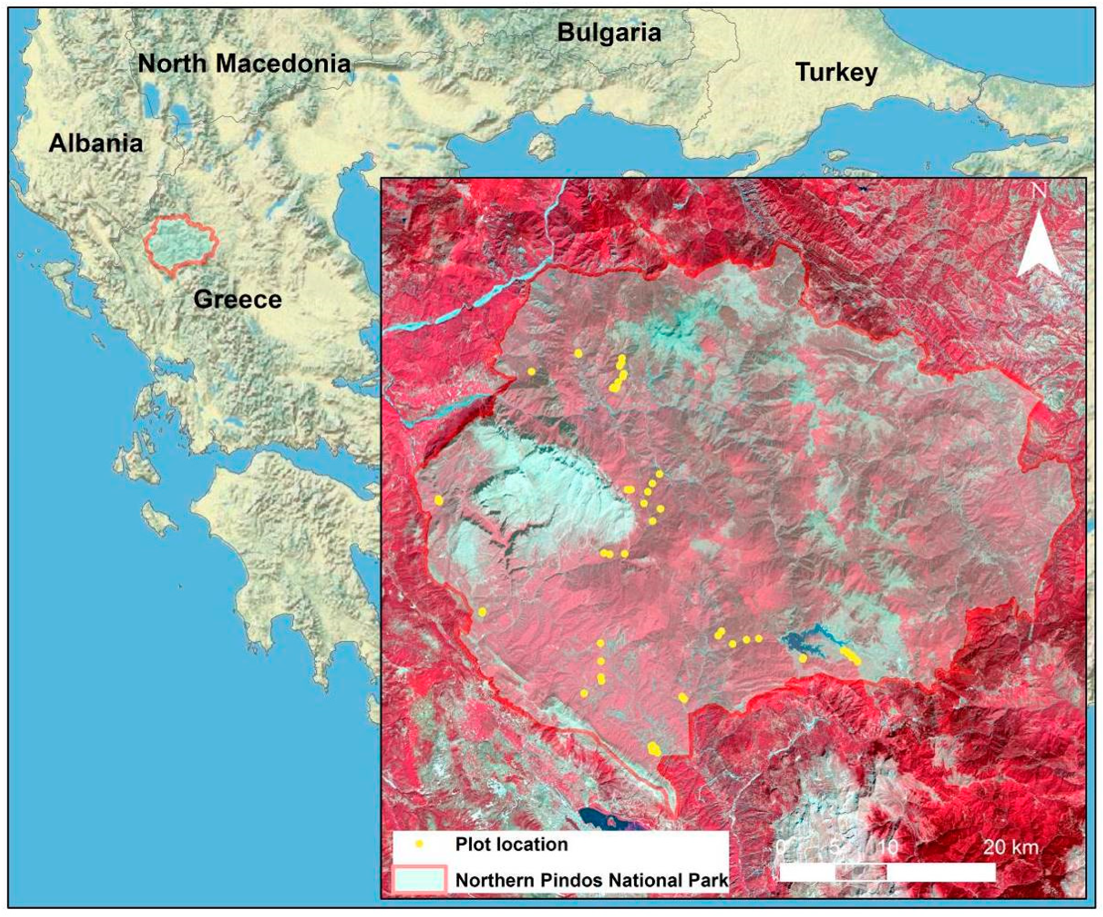
2.1. Study Area

The forest ecosystem under investigation is the Northern Pindos National Park, which is one of the largest protected terrestrial areas in Greece. The Park is located in Northwestern Greece and covers a total area 1969 sq. km. The region is characterized by a montane climate which varies in aspect and elevation. The annual precipitation ranges between 1000 and 1800 mm and the monthly temperatures average from 0.9 to 21.4 Celsius.
Northern Pindos National Park has an outstanding diversity of flora and fauna and the woodland covers a unique aesthetic landscape. Lower and middle altitudes are covered by oaks (Q. macedonica, Q. cerris, Q. pubescens, Quercus frainetto), and other mixed or pure stands of deciduous tree species (Ostrya carpinifolia, Carpinus orientalis, Carpinus betulus, Fraxinus ornus). At higher altitudes, two conifers Pinus nigra and Abies borissii regis are found. Up to 1800 m, beech forest (Fagus sylvatica) extends on the northern slopes, and Bosnian pine (Pinus leucodermis) covers the verge of the mountain slope. Above 1800 m, sub-alpine grasslands reach the peaks and often are dotted with Balkan pines (Pinus peuce). In the treeless alpine meadows, only certain types of scrubs are found.

2.2. Field Data

Field data were collected during August 2018. The set of ground data was constituted by 48 elementary sampling units (ESU) (Figure 1), where biophysical parameters were measured. Each ESU has a size equal to a pixel size (20 × 20 m) and were located among various forest types.
Canopy measurements were made with a portable photosynthetically active radiation meter ACCUPAR LP-80: PAR & LAI Ceptometer. The AccuPAR LP-80, facilitating non-destructive LAI measurements, consists of a linear array of 80 independent photosynthetically active radiation (PAR) sensors. The indirect field measurements with LP-80 AccuPAR Ceptometer consider the amount of light energy transmitted by a plant canopy and calculate LAI using a simplified version of the Norman–Jarvis radiation transmission and scattering model [36]. In each ESU, we collected above canopy measurements in nearby, unshaded open field, followed by six individual sensor retrievals below canopy, which were used to obtain a statistical mean of each ESU. The average LAI measures for broadleaved and coniferous species was 5.01 and 1.89, respectively.

2.3. Remote Sensing Data Acquisition and Preprocessing

The remotely sensing data employed in this study consist of a geometrically and atmospherically corrected at bottom-of-atmosphere (BoA) reflectance, and Sentinel-2 MSI (Level-2A) cloud-free image acquired on 25 August 2018. Sentinel imagery was available for download at no-cost via Sentinels Scientific Data Hub website (https://scihub.copernicus.eu/).
For the analysis, we retained 10 out of the 13 original spectral bands of the image (the 60 m spatial resolution bands were excluded), covering the visible to the shortwave infrared (SWIR) reflectance spectrum. The 10 m bands were resampled to 20 m to be compatible with the ESU size. Finally, three vegetation indices: normalized difference vegetation index (NDVI) [37], non-linear index (NLI) [38], and the normalized canopy index (NCI) [39], as well as their modified counterparts considering the red-edge and near-infrared regions of the spectrum [40,41], were estimated to generate the second feature set. In the second dataset, we also included the tasseled cap features (TCFs) [42] calculated upon the original spectral bands (Table 1).

2.4. Statistical Analysis

In the present study, a Gaussian process specified parametrically for regression problems was performed to determine the associations among field biophysical LAI measurements and spectral data. The Gaussian process is a Bayesian non-parametric algorithm, which could be considered as a generalization of a Gaussian (normal) probability distribution [43] extended to infinite dimensionality [44]. In contrast to other regression algorithms, the GPR algorithm does not define a conditional mean function but instead detects a befitting covariance between observations [45]. The GPR consists of a kernel method approach which can provide further advantages such as conditional, statistical information for the predicted variable. This extracted knowledge allows the interpretability as well as the flexibility of GPR models.
The GPR algorithm was used as implemented in the kernlab package [46] within the R environment software [47]. To assess the quality of the model, a 10-fold cross validation on the training data was performed. The determination coefficient (R2) and root mean square error (RMSE) were calculated to access the accuracy of the models. In general, the higher R2 values and the lower RMSE, the more accurate the model is. RMSE formula is:
R M S E = 1 n i = 1 n ( Y i ^ Y i ) 2
where n represents the number of predictions, Y ^ i is the prediction produced for observation i, and Y represents the observed values which are the inputs to the equation.
Initially, two GPR models (spectral bands and spectral indices) were developed using the full set of variables. In the next step, the importance of the individual predictors was estimated using permutation importance analysis. Permutation importance method figures the change in model’s performance before and after permuting the values of each variable and contrasts this to the predictions made on full dataset [48]. Using backward elimination selection technique [49] and gradually removing the least contributing variables, we established an adequate set of features as input for the new models.
Subsequently, the minimal subset of predictors producing the lowest RMSE and the best coefficient of determination (R2) for the LAI model were selected. The permutation importance analysis process was applied within R environment software (R Development Core Team, 2014) using ‘mlr’ package [48].

3. Results

Two GRP models for LAI prediction were built, considering the original ten spectral bands and the full set of spectral indices (Table 1). The accuracy of the spectral indices model was slightly better (R2 = 0.825 RMSE = 1.415) than that of the spectral bands model (R2 = 0.811 RMSE = 1.646) (Figure 2).
In the subsequent step of the analysis, we ranked the individual variables according to their importance on the model’s prediction performance. Figure 3 shows the permutation importance rankings for spectral bands and for the 16 spectral indices.
The most important variables in the spectral bands model were the SWIR (B11 and B12) and near infrared narrow band (NIRn1-B8A). The most important variables included in the spectral indices model were the NCI, the wetness (WET) and the modified NDVI index based on red-edge bands B5 and B6 (NDVI_RE1 and NDVI_RE2).
Figure 4 presents the results after the backward elimination and variable selection process. The highest performance for the spectral bands model was attained using seven spectral bands (R2 = 0.824 RMSE = 1.628). The variable selection procedure simplified the spectral indices model. The spectral indices model reached the highest accuracy (R2 = 0.854 and RMSE = 1.234) using five input variables (NCI2, NCI1, WET, NDVI_RE1, NDVI_RE2).
Finally, we produced LAI maps (Figure 5) based on the best developed models considering spectral bands and the spectral indices model.

4. Discussion

This study investigated the utility of Sentinel-2 spectral information for the estimation of the LAI over Northern Pindos National Park in Greece, using a GPR algorithm. As previous studies [29,50] have also indicated, the GPR technique provides a satisfactory accuracy of LAI estimates, efficiently handling a multi-dimensional dataset. In addition, GPR models generated through 10-fold cross validation on the training data reveal the most relevant variables to LAI in ranking order presenting an insight in the relation of LAI values with vegetation spectral response. The developed ranking list and the backward elimination process, pruning the least promising variables facilitated the development of less complex and computationally lighter model with less independent variables. and slightly improved accuracy.
The GPR model based on the original full dataset of spectral indices has shown marginally better performance than the model developed upon the spectral bands. The same pattern was also presented by the models after the variable selection procedure. Spectral indices models, using five spectral indices (NDVI, NLI, WET and the modified NLI_RE1, NLI_RE2) slightly outperformed the best spectral bands model of the seven spectral bands. In the Korhonen et al. [51] study, indices models present lower but adequate predictive accuracy compared to the individual band’s models, for the assessment of biophysical variables. In Verrelst et al.’s [33] study where CHRIS hyperspectral satellite images were used, the Gaussian Process model of four or more well chosen bands outperformed vegetation indices for the assessment of vegetation biophysical parameters. However, the measurement of LAI values in these previous studies referred to different biomes affecting the relationship with spectral response. It has to be also noted that even though several studies examined the relation between Earth observation data with LAI, the fact that different techniques and methods for LAI measures were applied in the field, may render them not comparable to one another.
Based on spectral bands’ importance rank order, SWIR (B11 and B12), NIRn2 (B8A), and NIR (B8) bands were found to be more proper for LAI assessment. Previous studies also found a strong correlation between SWIR bands with LAI [51,52]. Reflectance on the SWIR and NIR part of spectrum is noted to be affected by soil and vegetation attributes and thus can be useful for LAI estimation [53]. Moreover, the NIR as well the SWIR band has a capacity to sense plant components through combatively deep layers of vegetation [26,54]. In particular, the significance of the SWIR spectral band introduced by its relation to canopy reflectance and water content seems promising for the efficient estimation of LAI mostly in closed canopy forests [52]. The first narrow NIR B7 (NIRn1) and the second red-edge B6 (RE2) bands also appear to contribute importantly to LAI evaluation, as they are recognized indicators of plant chlorophyll content [55]. These bands located over the transition spectral zone which is characterized by chlorophyll absorption to leaf scattering, thus a positive change of leaf chlorophyll content implies reflectance changes from low in red-edge region to very high in the NIR [56].
Regarding the spectral indices importance rank order, the results were not entirely unexpected. NDVI is a very common index for LAI assessment across a wide range of ecosystems [51,52,57,58,59,60]. NDVI boosts the contrast between vegetation and soil but it minimizes the influence rising by illumination conditions [61]. In addition, NDVI is associated with well known limitations of saturation at intermediate levels of LAI [26]. The importance of NDVI for LAI estimation becomes weaker while LAI is increasing beyond a species-dependent threshold, which is commonly around mid-LAI values [57,62].
The modified versions of NDVI derived from the red-edge and near-infrared narrow bands are also among the high important variables. Twele et al. [63], who evaluated LAI in a tropical environment, found that the performance of indices using narrowband indices was better than that of broadband indices. Red edge has also been also by previous studies as a valuable variable for the assessment of LAI [51,55] due to its detection strength of canopy depth under dense canopy and high biomass status [64,65]. Meyer et al. [5] also indicated that vegetation indices developed on near-infrared bands were most highly correlated with LAI.
Furthermore, indices and TCFs have been suggested to avoid the saturation problem and enhance the predictive accuracies regarding forest LAI. Schönert et al. [66] confirmed the great abilities of TCFs for the estimation of crop LAI, using RapidEye imagery. The index of wetness, as also its terms reveals, gages the moisture content of the vegetation or soil by abstracting the sum of the visible and near infrared band from the longer infrared bands [67]. The wetness feature is sensitive to canopy moisture, thus as the amount of canopy increases, the wetness values rise until maximum canopy cover is achieved [67].
Moreover, the NCI index, which was calculated from the SWIR and green band, was presented as the most significant variable for LAI estimation. The importance of NCI for LAI assessment is linked to the green band’s sensitivity to chlorophyll and on SWIR sensitivity to moisture. In a dry rangeland ecosystem, Barati et al. [68] detected that NCI presented low prediction accuracy for biophysical parameters, compared to other vegetation indices. Vescovo et al. [39] found that NCI showed stronger correlation to LAI when phytomass levels were relatively high in a grassland environment. Consequently, according to these previous studies, the correlation strength of NCI with LAI depends on the biomass level. This fact is aligned with the results of our study where NCI is among the top ranking important variables for LAI estimation in a Mediterranean forest ecosystem.
All in all, the GPR algorithm, the variable selection technique, and the Sentinel-2 MSI spectral data seem appealing for LAI assessment over mixed Mediterranean forests. The achieved results could assist the efficient selection of proper Sentinel-2 MSI bands and spectral indices for LAI retrieval, in a regional setting approach and under an operational monitoring framework.
However, additional studies are required to establish the relation between the specific forest ecosystem attributes and biophysical parameters using optical remote sensing data, since environmental conditions affect the spectral response. Previous research has also highlighted the importance of the understory vegetation, species diversity, and surface moisture for modeling the LAI and spectral information linkage [69].

5. Conclusions

Remote sensing-based LAI measurements could be used to monitor forest ecosystems response to the pressures induced by various drivers of change, and to indicate early warning signs regarding forest sustainability risks. In this paper, we evaluated the utility of Sentinel-2 MSI satellite imagery for estimating LAI in a heterogenous Mediterranean forest. Furthermore, we compared the effectiveness of spectral indices and the spectral band to model LAI using the GPR algorithm and we identified the most relevant informative variables for monitoring and mapping LAI.
The results of the present study can be summarized as follows:
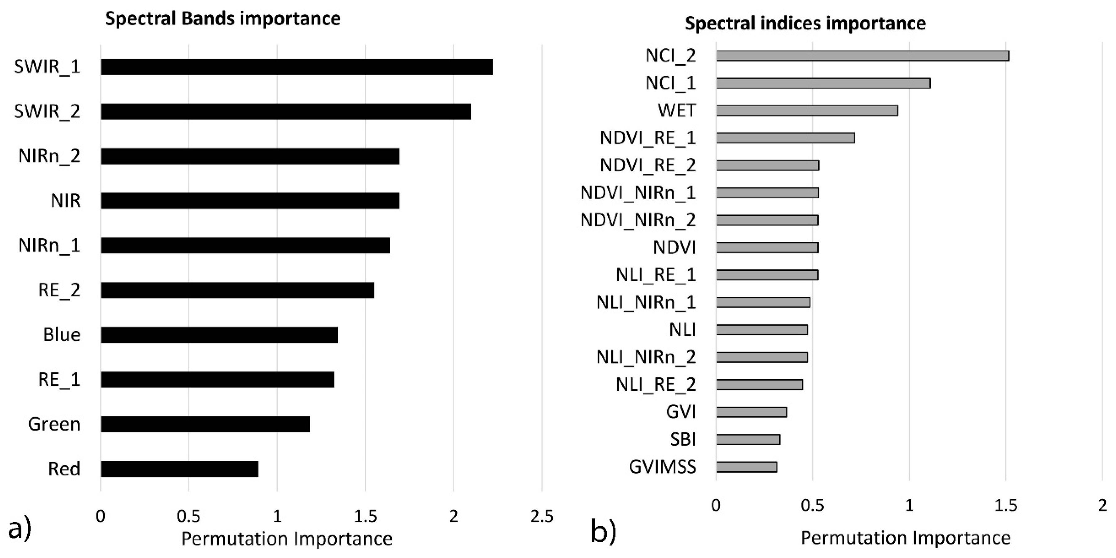
GRP algorithm seems promising for LAI estimation and LAI models’ interpretation through variables’ permutation importance rankings;
Although SWIR bands have been designed for atmospheric correction applications and supposed to be of mirror significance for biophysical parameter estimation, GPR revealed spectral information in SWIR bands which is proven to be beneficial for the assessment of biophysical parameter such as LAI;
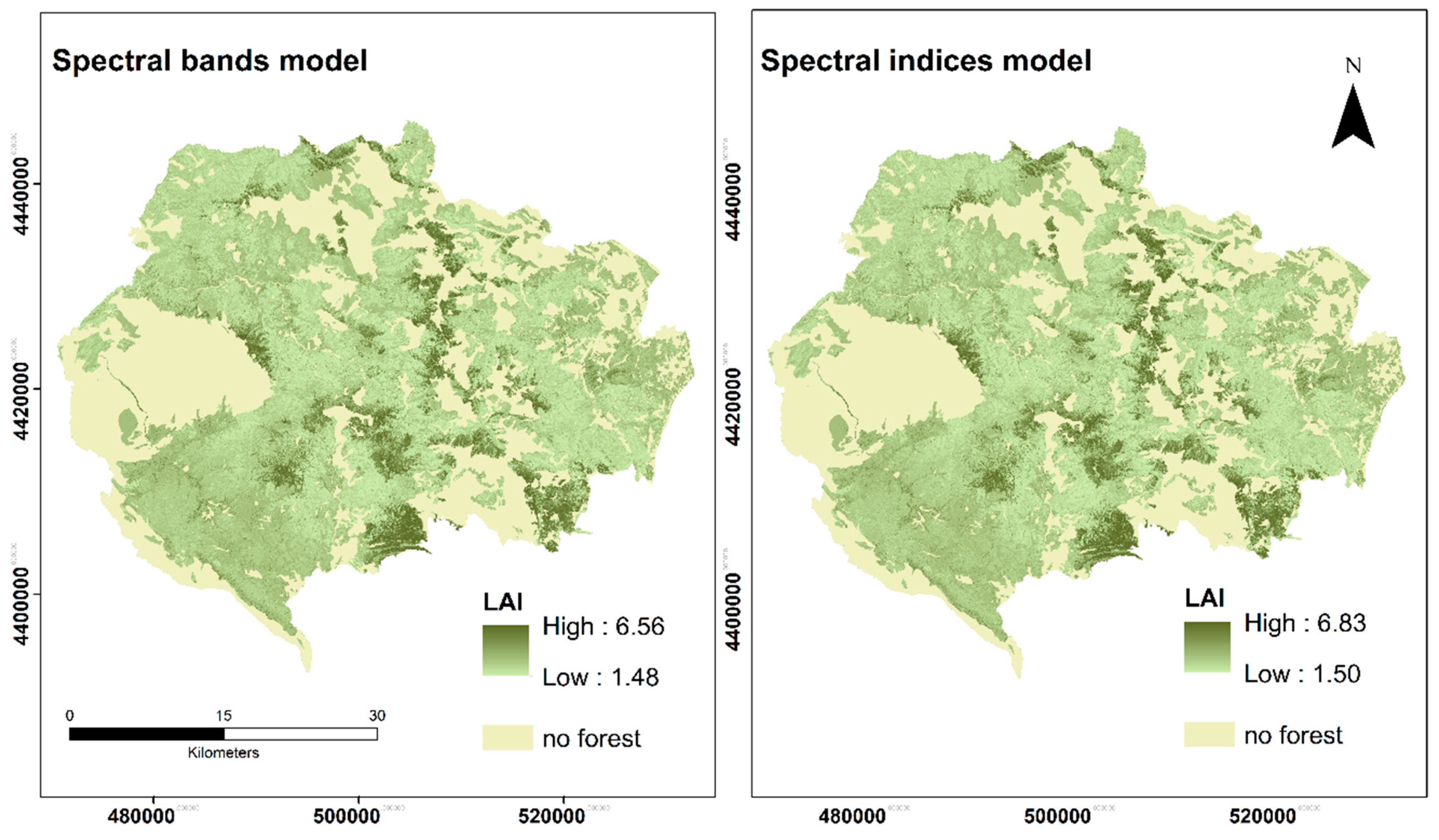
LAI over a heterogeneous Mediterranean forest can be mapped at a high predictive accuracy using five spectral indices (NCI2, NCI1, WET, NDVI_RE1, NDVI_RE2). NCI, red-edge NDVI, and TCFs wetness indices have been proven to be important predictors for forest LAI modeling.
Overall, the outcomes of this research provide proof of the potential of Sentinel-2 MSI spectral resolution for LAI assessment in Mediterranean forests. However, additional sampling efforts, extended over several growing seasons, could contribute in the verifying the robustness of our findings.

Author Contributions

Conceptualization, G.M.; methodology, I.C. and G.M.; investigation, G.M., I.C., G.K.; data analysis, I.C.; writing—original draft preparation, I.C. and G.M.; review and editing, I.C., G.M., G.K., A.P.K.; supervision, G.M. All authors have read and agreed to the published version of the manuscript.

Funding

This research was funded by the project “Conservation and sustainable capitalization of biodiversity in forested areas-BIOPROSPECT” (Reg. No: BMP1/2.1/2336/2017), implemented within the framework of INTERREG V-A COOPERATION PROGRAMME BALKAN MEDITERRANEAN 2014–2020 programme, co-funded by the European Union and national funds of the participating countries.

Acknowledgments

The Sentinel-2 MSI data were available from the European Space Agency at no-cost. The authors are grateful to Athanasios Stampoulidis and the staff of the Northern Pindos National Park Management Body for their help during field sampling activities.

Conflicts of Interest

The authors declare no conflict of interest.

References

  1. Asner, G.P.; Scurlock, J.M.O.; Hicke, J.A. Global synthesis of leaf area index observations: Implications for ecological and remote sensing studies. Glob. Ecol. Biogeogr. 2003, 12, 191–205. [Google Scholar] [CrossRef] [Green Version]
  2. Yan, G.; Hu, R.; Luo, J.; Weiss, M.; Jiang, H.; Mu, X.; Xie, D.; Zhang, W. Review of indirect optical measurements of leaf area index: Recent advances, challenges, and perspectives. Agric. For. Meteorol. 2019, 265, 390–411. [Google Scholar] [CrossRef]
  3. Dash, J.; Ogutu, B.O. Recent advances in space-borne optical remote sensing systems for monitoring global terrestrial ecosystems. Prog. Phys. Geogr. Earth Environ. 2016, 40, 322–351. [Google Scholar] [CrossRef]
  4. Brede, B.; Verrelst, J.; Gastellu-Etchegorry, J.-P.; Clevers, J.G.P.W.; Goudzwaard, L.; den Ouden, J.; Verbesselt, J.; Herold, M. Assessment of Workflow Feature Selection on Forest LAI Prediction with Sentinel-2A MSI, Landsat 7 ETM+ and Landsat 8 OLI. Remote Sens. 2020, 12, 915. [Google Scholar] [CrossRef] [Green Version]
  5. Meyer, L.H.; Heurich, M.; Beudert, B.; Premier, J.; Pflugmacher, D. Comparison of Landsat-8 and Sentinel-2 Data for Estimation of Leaf Area Index in Temperate Forests. Remote Sens. 2019, 11, 1160. [Google Scholar] [CrossRef] [Green Version]
  6. Pope, G.; Treitz, P. Leaf Area Index (LAI) estimation in boreal mixedwood forest of Ontario, Canada using Light detection and ranging (LiDAR) and worldview-2 imagery. Remote Sens. 2013, 5, 5040–5063. [Google Scholar] [CrossRef] [Green Version]
  7. Gower, S.T.; Kucharik, C.J.; Norman, J.M. Direct and Indirect Estimation of Leaf Area Index, fAPAR, and Net Primary Production of Terrestrial Ecosystems. Remote Sens. Environ. 1999, 70, 29–51. [Google Scholar] [CrossRef]
  8. Brown, L.A.; Ogutu, B.O.; Dash, J. Estimating Forest Leaf Area Index and Canopy Chlorophyll Content with Sentinel-2: An Evaluation of Two Hybrid Retrieval Algorithms. Remote Sens. 2019, 11, 1752. [Google Scholar] [CrossRef] [Green Version]
  9. Zheng, G.; Moskal, L.M. Retrieving Leaf Area Index (LAI) Using Remote Sensing: Theories, Methods and Sensors. Sensors 2009, 9, 2719–2745. [Google Scholar] [CrossRef] [Green Version]
  10. Fang, H.; Liang, S. Leaf Area Index Models. In Reference Module in Earth Systems and Environmental Sciences; Elsevier: Amsterdam, The Netherlands, 2014; ISBN 978-0-12-409548-9. [Google Scholar]
  11. Song, C. Optical remote sensing of forest leaf area index and biomass. Prog. Phys. Geogr. 2012, 37, 98–113. [Google Scholar] [CrossRef]
  12. Liu, K.; Zhou, Q.; Wu, W.; Xia, T.; Tang, H. Estimating the crop leaf area index using hyperspectral remote sensing. J. Integr. Agric. 2016, 15, 475–491. [Google Scholar] [CrossRef] [Green Version]
  13. Liang, L.; Qin, Z.; Zhao, S.; Di, L.; Zhang, C.; Deng, M.; Lin, H.; Zhang, L.; Wang, L.; Liu, Z. Estimating crop chlorophyll content with hyperspectral vegetation indices and the hybrid inversion method. Int. J. Remote Sens. 2016, 37, 2923–2949. [Google Scholar] [CrossRef]
  14. Kimes, D.S.; Knyazikhin, Y.; Privette, J.L.; Abuelgasim, A.A.; Gao, F. Inversion methods for physically-based models. Remote Sens. Rev. 2000, 18, 381–439. [Google Scholar] [CrossRef]
  15. Sun, Y.; Qin, Q.; Ren, H.; Zhang, T.; Chen, S. Red-Edge Band Vegetation Indices for Leaf Area Index Estimation From Sentinel-2/MSI Imagery. IEEE Trans. Geosci. Remote Sens. 2020, 58, 826–840. [Google Scholar] [CrossRef]
  16. Cohrs, C.W.; Cook, R.L.; Gray, J.M.; Albaugh, T.J. Sentinel-2 Leaf Area Index Estimation for Pine Plantations in the Southeastern United States. Remote Sens. 2020, 12, 1406. [Google Scholar] [CrossRef]
  17. Siachalou, S.; Mallinis, G.; Tsakiri-Strati, M. Analysis of Time-Series Spectral Index Data to Enhance Crop Identification Over a Mediterranean Rural Landscape. IEEE Geosci. Remote Sens. Lett. 2017, 14, 1508–1512. [Google Scholar] [CrossRef]
  18. Kalacska, M.; Sanchez-Azofeifa, G.A.; Caelli, T.; Rivard, B.; Boerlage, B. Estimating leaf area index from satellite imagery using Bayesian networks. IEEE Trans. Geosci. Remote Sens. 2005, 43, 1866–1873. [Google Scholar] [CrossRef]
  19. Pu, R.; Gong, P.; Biging, G.S.; Larrieu, M.R. Extraction of red edge optical parameters from Hyperion data for estimation of forest leaf area index. IEEE Trans. Geosci. Remote Sens. 2003, 41, 916–921. [Google Scholar]
  20. Omer, G.; Mutanga, O.; Abdel-Rahman, E.M.; Adam, E. Empirical prediction of leaf area index (LAI) of endangered tree species in intact and fragmented indigenous forests ecosystems using WorldView-2 data and two robust machine learning algorithms. Remote Sens. 2016, 8, 324. [Google Scholar] [CrossRef] [Green Version]
  21. Durbha, S.S.; King, R.L.; Younan, N.H. Support vector machines regression for retrieval of leaf area index from multiangle imaging spectroradiometer. Remote Sens. Environ. 2007, 107, 348–361. [Google Scholar] [CrossRef]
  22. Wang, J.; Xiao, X.; Bajgain, R.; Starks, P.; Steiner, J.; Doughty, R.B.; Chang, Q. Estimating leaf area index and aboveground biomass of grazing pastures using Sentinel-1, Sentinel-2 and Landsat images. ISPRS J. Photogramm. Remote Sens. 2019, 154, 189–201. [Google Scholar] [CrossRef] [Green Version]
  23. Wang, L.; Chang, Q.; Yang, J.; Zhang, X.; Li, F. Estimation of paddy rice leaf area index using machine learning methods based on hyperspectral data from multi-year experiments. PLoS ONE 2018, 13, e0207624. [Google Scholar] [CrossRef] [PubMed] [Green Version]
  24. Xiao, Z.; Liang, S.; Wang, T.; Jiang, B. Retrieval of leaf area index (LAI) and fraction of absorbed photosynthetically active radiation (FAPAR) from VIIRS time-series data. Remote Sens. 2016, 8, 351. [Google Scholar] [CrossRef] [Green Version]
  25. Kiala, Z.; Odindi, J.; Mutanga, O. Potential of interval partial least square regression in estimating leaf area index. S. Afr. J. Sci. 2017, 113, 1–9. [Google Scholar] [CrossRef]
  26. Houborg, R.; McCabe, M.F. A hybrid training approach for leaf area index estimation via Cubist and random forests machine-learning. ISPRS J. Photogramm. Remote Sens. 2018, 135, 173–188. [Google Scholar] [CrossRef]
  27. Campos-Taberner, M.; García-Haro, F.J.; Camps-Valls, G.; Grau-Muedra, G.; Nutini, F.; Crema, A.; Boschetti, M. Multitemporal and multiresolution leaf area index retrieval for operational local rice crop monitoring. Remote Sens. Environ. 2016, 187, 102–118. [Google Scholar] [CrossRef]
  28. Verrelst, J.; Rivera, J.P.; Gitelson, A.; Delegido, J.; Moreno, J.; Camps-Valls, G. Spectral band selection for vegetation properties retrieval using Gaussian processes regression. Int. J. Appl. Earth Obs. Geoinf. 2016, 52, 554–567. [Google Scholar] [CrossRef]
  29. Verrelst, J.; Rivera, J.P.; Veroustraete, F.; Muñoz-Marí, J.; Clevers, J.G.P.W.; Camps-Valls, G.; Moreno, J. Experimental Sentinel-2 LAI estimation using parametric, non-parametric and physical retrieval methods—A comparison. ISPRS J. Photogramm. Remote Sens. 2015, 108, 260–272. [Google Scholar] [CrossRef]
  30. Ali, A.M.; Darvishzadeh, R.; Skidmore, A.; Gara, T.W.; Heurich, M. Machine learning methods’ performance in radiative transfer model inversion to retrieve plant traits from Sentinel-2 data of a mixed mountain forest. Int. J. Digit. Earth 2020, 1–15. [Google Scholar] [CrossRef]
  31. Svendsen, D.H.; Morales-Álvarez, P.; Ruescas, A.B.; Molina, R.; Camps-Valls, G. Deep Gaussian processes for biogeophysical parameter retrieval and model inversion. ISPRS J. Photogramm. Remote Sens. 2020, 166, 68–81. [Google Scholar] [CrossRef]
  32. Camps-Valls, G.; Sejdinovic, D.; Runge, J.; Reichstein, M. A perspective on Gaussian processes for Earth observation. Natl. Sci. Rev. 2019, 6, 616–618. [Google Scholar] [CrossRef] [Green Version]
  33. Verrelst, J.; Alonso, L.; Camps-valls, G.; Member, S.; Delegido, J.; Moreno, J. Retrieval of Vegetation Biophysical Parameters Using Gaussian Process Techniques. IEEE Trans. Geosci. Remote Sens. 2012, 50, 1832–1843. [Google Scholar] [CrossRef]
  34. Pasolli, L.; Melgani, F.; Blanzieri, E. Estimating Biophysical Parameters from remotely sensed imagery with gaussian processes. In Proceedings of the IGARSS 2008 IEEE International Geoscience and Remote Sensing Symposium, Boston, MA, USA, 7–11 July 2008; pp. 851–854. [Google Scholar]
  35. Camps-Valls, G.; Verrelst, J.; Munoz-Mari, J.; Laparra, V.; Mateo-Jimenez, F.; Gomez-Dans, J. A Survey on Gaussian Processes for Earth-Observation Data Analysis: A Comprehensive Investigation. IEEE Geosci. Remote Sens. Mag. 2016, 4, 58–78. [Google Scholar] [CrossRef] [Green Version]
  36. Pokovai, K.; Fodor, N. Adjusting Ceptometer Data to Improve Leaf Area Index Measurements. Agronomy 2019, 9, 866. [Google Scholar] [CrossRef] [Green Version]
  37. Rouse, J.W.; Haas, R.H.; Schell, J.A.; Deering, D.W. Monitoring the vernal advancement and retrogradation (green wave effect) of natural vegetation. In Final Report, RSC 1978–4, Texas A M Univ Coll Station Texas; NASA: Washington, DC, USA, 1973. [Google Scholar]
  38. Goel, N.S.; Qin, W. Influences of canopy architecture on relationships between various vegetation indices and LAI and FPAR: A computer simulation. Remote Sens. Rev. 1994, 10, 309–347. [Google Scholar] [CrossRef]
  39. Vescovo, L.; Gianelle, D. Using the MIR bands in vegetation indices for the estimation of grassland biophysical parameters from satellite remote sensing in the Alps region of Trentino (Italy). Adv. Space Res. 2008, 41, 1764–1772. [Google Scholar] [CrossRef]
  40. Chrysafis, I.; Mallinis, G.; Tsakiri, M.; Patias, P. Evaluation of single-date and multi-seasonal spatial and spectral information of Sentinel-2 imagery to assess growing stock volume of a Mediterranean forest. Int. J. Appl. Earth Obs. Geoinf. 2019, 77, 1–14. [Google Scholar] [CrossRef]
  41. Chrysafis, I.; Mallinis, G.; Siachalou, S.; Patias, P. Assessing the relationships between growing stock volume and Sentinel-2 imagery in a Mediterranean forest ecosystem. Remote Sens. Lett. 2017, 8, 508–517. [Google Scholar] [CrossRef]
  42. Henrich, V.; Jung, A.; Götze, C.; Sandow, C.; Thürkow, D.; Gläßer, C. Development of an online indices database: Motivation, concept and implementation. In Proceedings of the 6th EARSeL Imaging Spectroscopy SIG Workshop Innovative Tool for Scientific and Commercial Environment Applications, Tel Aviv, Israel, 16–18 March 2009. [Google Scholar]
  43. Kocijan, J.; Murray-Smith, R.; Rasmussen, C.E.; Likar, B. Predictive control with Gaussian process models. In Proceedings of the IEEE Region 8 EUROCON 2003. Computer as a Tool, Ljubljana, Slovenia, 22–24 September 2003. [Google Scholar]
  44. Ebden, M. Gaussian Processes: A Quick Introduction. arXiv 2015, arXiv:1505.02965. [Google Scholar]
  45. Mehdipour, P.; Navidi, I.; Parsaeian, M.; Mohammadi, Y.; Moradi Lakeh, M.; Rezaei Darzi, E.; Nourijelyani, K.; Farzadfar, F. Application of Gaussian Process Regression (GPR) in estimating under-five mortality levels and trends in Iran 1990–2013, study protocol. Arch. Iran. Med. 2014, 17, 189–192. [Google Scholar]
  46. Karatzoglou, A.; Smola, A.; Hornik, K.; Zeileis, A. kernlab-An S4 Package for Kernel Methods in R. J. Stat. Softw. 2004, 11, 1–20. [Google Scholar] [CrossRef] [Green Version]
  47. R Development Core Team R. A Language and Environment for Statistical Computing. R Found. Stat. Comput. 2014, 1, 409. [Google Scholar]
  48. Bischl, B.; Lang, M.; Kotthoff, L.; Schiffner, J.; Richter, J.; Studerus, E.; Casalicchio, G.; Jones, Z.M. mlr: Machine Learning in R. J. Mach. Learn. Res. 2016, 17, 1–5. [Google Scholar]
  49. Polak, P.; Karlić, R.; Koren, A.; Thurman, R.; Sandstrom, R.; Lawrence, M.S.; Reynolds, A.; Rynes, E.; Vlahoviček, K.; Stamatoyannopoulos, J.A.; et al. Cell-of-origin chromatin organization shapes the mutational landscape of cancer. Nature 2015, 518, 360–364. [Google Scholar] [CrossRef] [PubMed]
  50. Campos-Taberner, M.; García-Haro, F.J.; Busetto, L.; Ranghetti, L.; Martínez, B.; Gilabert, M.A.; Camps-Valls, G.; Camacho, F.; Boschetti, M. A critical comparison of remote sensing Leaf Area Index estimates over rice-cultivated areas: From Sentinel-2 and Landsat-7/8 to MODIS, GEOV1 and EUMETSAT polar system. Remote Sens. 2018, 10, 763. [Google Scholar] [CrossRef] [Green Version]
  51. Korhonen, L.; Hadi; Packalen, P.; Rautiainen, M. Comparison of Sentinel-2 and Landsat 8 in the estimation of boreal forest canopy cover and leaf area index. Remote Sens. Environ. 2017, 195, 259–274. [Google Scholar] [CrossRef]
  52. Lee, K.S.; Park, Y.I.; Kim, S.H.; Park, J.H.; Woo, C.S.; Jang, K.C. Remote sensing estimation of forest LAI in close canopy situation. Int. Arch. Photogramm. Remote Sens. Spat. Inf. Sci. -ISPRS Arch. 2004, 35. [Google Scholar]
  53. Bannari, A.; Pacheco, A.; Staenz, K.; McNairn, H.; Omari, K. Estimating and mapping crop residues cover on agricultural lands using hyperspectral and IKONOS data. Remote Sens. Environ. 2006, 104, 447–459. [Google Scholar] [CrossRef]
  54. Lillesaeter, O. Spectral reflectance of partly transmitting leaves: Laboratory measurements and mathematical modeling. Remote Sens. Environ. 1982, 12, 247–254. [Google Scholar] [CrossRef]
  55. Filella, I.; Penuelas, J. The red edge position and shape as indicator of plant chlorophyll content, biomass and hydric status. Int. J. Remote Sens. 1994, 15, 1459–1470. [Google Scholar] [CrossRef]
  56. Delegido, J.; Verrelst, J.; Meza, C.M.; Rivera, J.P.; Alonso, L.; Moreno, J. A red-edge spectral index for remote sensing estimation of green LAI over agroecosystems. Eur. J. Agron. 2013, 46, 42–52. [Google Scholar] [CrossRef]
  57. Davi, H.; Soudani, K.; Deckx, T.; Dufrene, E.; Le Dantec, V.; François, C. Estimation of forest leaf area index from SPOT imagery using NDVI distribution over forest stands. Int. J. Remote Sens. 2006, 27, 885–902. [Google Scholar] [CrossRef]
  58. Gong, P.; Pu, R.; Biging, G.S.; Larrieu, M.R. Estimation of forest leaf area index using vegetation indices derived from Hyperion hyperspectral data. IEEE Trans. Geosci. Remote Sens. 2003, 41, 1355–1362. [Google Scholar] [CrossRef] [Green Version]
  59. Onojeghuo, A.O.; Blackburn, G.A. Understanding the multi-seasonal spectral and biophysical characteristics of reedbed habitats in the UK. Geospat. Inf. Sci. 2016, 19, 233–244. [Google Scholar] [CrossRef] [Green Version]
  60. Houborg, R.; McCabe, M.F. Daily retrieval of NDVI and LAI at 3 m resolution via the fusion of CubeSat, Landsat, and MODIS data. Remote Sens. 2018, 10, 890. [Google Scholar] [CrossRef] [Green Version]
  61. Baret, F.; Guyot, G. Potentials and limits of vegetation indices for LAI and APAR assessment. Remote Sens. Environ. 1991, 35, 161–173. [Google Scholar] [CrossRef]
  62. Wang, F.; Huang, J.; Tang, Y.; Wang, X. New Vegetation Index and Its Application in Estimating Leaf Area Index of Rice. Rice Sci. 2007, 14, 195–203. [Google Scholar] [CrossRef]
  63. Twele, A.; Erasmi, S.; Kappas, M. Spatially Explicit Estimation of Leaf Area Index Using EO-1 Hyperion and Landsat ETM+ Data: Implications of Spectral Bandwidth and Shortwave Infrared Data on Prediction Accuracy in a Tropical Montane Environment. GISci. Remote Sens. 2008, 45, 229–248. [Google Scholar] [CrossRef]
  64. Ciganda, V.S.; Gitelson, A.A.; Schepers, J. How deep does a remote sensor sense? Expression of chlorophyll content in a maize canopy. Remote Sens. Environ. 2012, 126, 240–247. [Google Scholar] [CrossRef]
  65. Feng, W.; Wu, Y.; He, L.; Ren, X.; Wang, Y.; Hou, G.; Wang, Y.; Liu, W.; Guo, T. An optimized non-linear vegetation index for estimating leaf area index in winter wheat. Precis. Agric. 2019, 20, 1157–1176. [Google Scholar] [CrossRef] [Green Version]
  66. Schönert, M.; Zillmann, E.; Weichelt, H.; Eitel, J.U.H.; Magney, T.S.; Lilienthal, H.; Siegmann, B.; Jarmer, T. The tasseled cap transformation for RapidEye data and the estimation of vital and senescent crop parameters. Int. Arch. Photogramm. Remote Sens. Spat. Inf. Sci. ISPRS Arch. 2015, 40, 101–108. [Google Scholar] [CrossRef] [Green Version]
  67. Lea, R.D.; Cowell, C.M.; Supervisor, T. A Comparison of Forest Change Detection Methods and Implications for Forest Management. Master’s Thesis, University of Missouri-Columbia, Columbia, MO, USA, 2005. [Google Scholar]
  68. Barati, S.; Rayegani, B.; Saati, M.; Sharifi, A.; Nasri, M. Comparison the accuracies of different spectral indices for estimation of vegetation cover fraction in sparse vegetated areas. Egypt. J. Remote Sens. Space Sci. 2011, 14, 49–56. [Google Scholar] [CrossRef] [Green Version]
  69. Eklundh, L.; Hall, K.; Eriksson, H.; Ardö, J.; Pilesjö, P. Investigating the use of landsat thematic mapper data for estimation of forest leaf area index in southern Sweden. Can. J. Remote Sens. 2003, 29, 349–362. [Google Scholar] [CrossRef] [Green Version]
Figure 1. Study area and field plot location overlaid on a Sentinel-2 image (red: near infrared 2; green: red; blue: green).
Ijgi 09 00622 g001
Figure 2. The relationship between the observed and predicted values of (a) the spectral bands model and (b) the spectral indices model on the full dataset.
Ijgi 09 00622 g002
Figure 3. The most important predictor variables in rank order, using the permutation importance of (a) spectral bands and (b) spectral indices datasets.
Ijgi 09 00622 g003
Figure 4. (a) The optimal predictive variable selection using the backward elimination process. (b) Relationships between the predictive and actual LAI values, using the best spectral bands and spectral indices model. Points represent measurements at the ESU level, dashed lines represent a 1:1 relationship.
Ijgi 09 00622 g004
Figure 5. Leaf area index (LAI) maps based on Sentinel-2 (left) spectral bands and (right) spectral indices best prediction models.
Ijgi 09 00622 g005
Table 1. Spectral Variables used in the present study.
Sentinel-2 Spectral BandsSentinel-2 Spectral Indices
B2—BlueBlueNon-linear index NLI   = NIR 2 Red NIR 2 + Red
B3—GreenGreenNon-linear index red-edge 1 NLI RE 1 = RE 1 2 Red RE 1 2 + Red
B4—RedRedNon-linear index red-edge 2 NLI RE 2 = RE 2 2 Red RE 2 2 + Red
B5—Red Edge 1RE1Non-linear index near-infrared 1 NLI NIR n 1 = NIR n 1 2 Red NIR n 1 2 + Red
B6—Red Edge 2RE2Non-linear index near-infrared 2 NLI NIR n 2 = NIR n 2 2 Red NIR n 2 2 + Red
B7—Near Infrared narrow 1NIRn1Normalized difference vegetation index N D V I = N I R R e d N I R + R e d
B8—Near Infrared NIRNDVI red-edge 1 N D V I = R E 1 R e d R E 1 + R e d
B8a—Near Infrared narrow 2NIRn2NDVI red-edge 2 NDVI RE 2 = RE 2 Red RE 2 + Red
B11—Short Wave InfraRed 1SWIR 1NDVI near-infrared 1 NDVI NIR n 1 = NIR n 1 Red NIR n 1 + Red
B12—Short Wave InfraRed 2SWIR 2NDVI near-infrared 2 NDVI NIR n 2 = NIR n 2 Red NIR n 2 + Red
Normalized canopy index 1 NCI 1 = SWIR 1 Green SWIR 1 + Green
Normalized canopy index 2 NCI 2 = SWIR 2 Green SWIR 2 + Green
Tasseled Cap Features (TCFs)
Wetness WET = 0.1509 × Blue + 0.1973 × Green + 0.3279 × Red + 0.3406 × NIR 0.7112 × SWIR 1 0.4572 × SWIR 2
Vegetation GVI = 02848 × Blue 0.2435 × Green 0.5436 × Red + 0.7243 × NIR + 0.084 × SWIR 1 0.18 × SWIR 2
Brightness SBI   = 0.3037 × Blue + 0.2793 × Green + 0.4743 × Red + 0.5585 × NIR + 0.5082 × SWIR 1 + 0.1863 × SWIR 2
Green vegetation index MSS GVIMSS   = 0.283 × Green 0.66 × Red + 0.577 × RE 2 + 0.388 × NIR
Publisher’s Note: MDPI stays neutral with regard to jurisdictional claims in published maps and institutional affiliations.

