Workflow of Digital Field Mapping and Drone-Aided Survey for the Identification and Characterization of Capable Faults: The Case of a Normal Fault System in the Monte Nerone Area (Northern Apennines, Italy)

Abstract

Field work on the search and characterization of ground effects of a historical earthquake (i.e., the Cagli earthquake in 1781) was carried out using terrestrial and aerial digital tools. The method of capturing, organizing, storing, and elaborating digital data is described herein, proposing a possible workflow starting from pre-field project organization, through reiteration of field and intermediate laboratory work, to final interpretation and synthesis. The case of one of the most important seismic events in the area of the northern Umbria–Marche Apennines provided the opportunity to test the method with both postgraduate students and researchers. The main result of this work was the mapping of a capable normal fault system with a great number of observations, as well as a large amount of data, from difficult outcrop areas. A GIS map and a three-dimensional (3D) model, with the integration of subsurface data (i.e., seismic profiles and recent earthquake distribution information), allowed for a new interpretation of an extensional tectonic regime of this Apennines sector, similar to one of the southernmost areas of central Italy where recent earthquakes occurred on 2016.

1. Introduction

The research and mapping of faults and ground deformation are fundamental for seismic characterization of tectonically active areas. To this end, a lot of work has been carried out in various regions around the world, such as in Italy after the occurrence of the latest earthquakes (i.e., in L’Aquila in 2009, in central Italy in 2016, and in Ischia in 2017). Geologists and geophysicists use digital devices and tools to minimize time and errors, thus increasing the accuracy of data and observations [1,2,3,4,5,6,7,8,9,10]. Indeed, these methods have been applied to active fault characterization of recent seismic events, that is, events that occurred a few years prior to the characterization (i.e., in L’Aquila in 2009 and in central Italy in 2016), where traces of the co-seismic effects are still evident and well preserved.

In this study, we applied digital survey methods to investigate an area where a historical seismic event occurred. On 3 June 1781, a strong earthquake (6.5 Mw) [11] affected the northern sector of the Umbria–Marche Apennines [12,13]. The disaster generated by this event was reported in many archival documents at the time [14]. Despite the importance of the occurrence of similar seismic events, very little is known about the tectonic and structural features related to the 1781 event, even though some hypotheses regarding its kinematics have been formulated [15,16].

To the best of the authors’ knowledge, no field studies of this scope have been carried out previously. After more than two centuries, most of the ground deformation features would have been disturbed or completely destroyed by vegetation growth, natural erosion, and anthropic activities. In such cases, it is extremely difficult to find explicit evidence to unequivocally link outcropping faults to an earthquake event. However, being a populated area, the characterization of an event that could reoccur in the future is crucial for the safety and economy of this seismically active Apennine sector.

1.1. Tectonic Lineaments

The Umbro–Marche Apennines are located in the outer part of the orogenic chain of northern Apennines (Figure 1). The rotation of the Sardinian–Corsica block toward the Adriatic foreland created a thrust belt chain of tectonic units and thrust systems that have been migrating since Oligocene to Pliocene–Quaternary times from the inner Tyrrhenian side to the external Adriatic side [17,18]. The building of the orogenic chain was followed by a progressive extensional phase always in the NE–SW direction and always in the same direction [19]. Therefore, in the Tyrrhenian Tuscan–Umbrian sector, the compressive structures are cut by subsequent normal faults, while in the Adriatic region, a compression regime persists; the Apennines watershed represents the boundary between extensional and compressional regimes [20].

More recently, some authors believe that the extensional regime is not confined in the west of the Apennine watershed, and that evidence of this extensional tectonics can even be found toward the east [21,22,23]. Moreover, a low-angle normal fault (LANF) [24,25] dipping eastward, toward the foreland, has been interpreted in deep seismic profiles [18]. Therefore, the seismic events recorded in this area could be related to this fault [26,27].

These tectonic structures are potentially active, as indicated by several authors [28,29,30]. In this context, the aim of this research was to investigate faults capable of generating seismic events comparable to that of the 1781 earthquake with the highest estimated magnitude in this area.

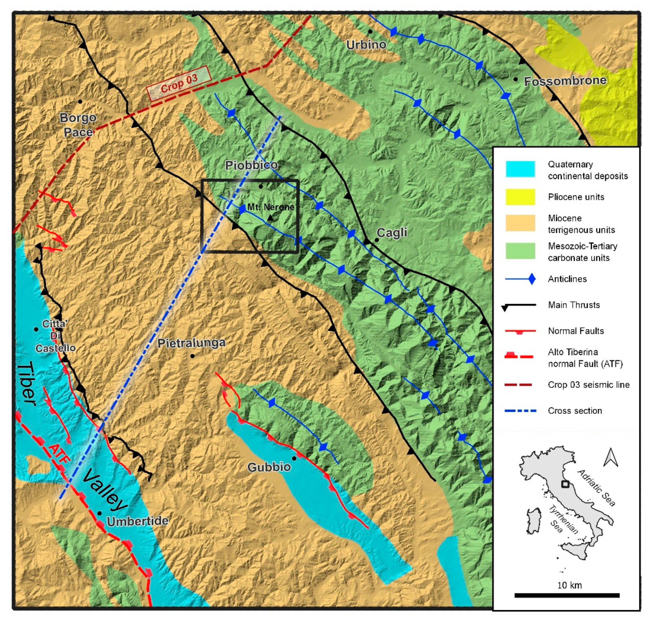
1.2. Geological Settings of the Study Area

The study area was part of the inner sector of the Umbro–Marche Apennines (Pesaro and Urbino Province, northern Marche), in the area of Monte Nerone and its southeastward extension (Figure 2). Here, a carbonate succession ranges from the Lower Jurassic to Oligocene outcrops [31]. It was deposited in a basin at the edge of the African platform during the transition from the Liassic rifting to drifting and the development of the passive margin [32]. Upsection, the increase in the terrigenous fine sediment content in the succession (Scaglie group) represents a transition toward the succession of a mainly turbiditic complex of Miocenic foredeep [33,34].

The local geological structure is an anticlinorium with an emi-wavelength of 5–6 km and a longitudinal extension of more than 30 km. This anticlinorium is oriented NW–SE, consistent with the typical fold-and-thrust structure orientation in the northern Apennines.

The anticlinorium is dissected by a set of WNW–ESE trending faults, possibly with normal movements. Less pervasive ENE–WSW-oriented faults, limited to the western portion of the mapped area, exibit transcurrent movements. The longitudinal extent of the faults, of both WNW–ESE and ENE–WSW trends, is reduced by approximately 1 km, while there is no obvious, unequivocal aggregation of these fault segments into larger structures.

1.3. Aims

This article describes and proposes a methodological workflow for the characterization of an active fault system including (i) field research based on digital ground and aerial surveys, (ii) laboratory analyses, and (iii) data interpretation and synthesis (Figure 3).

We demonstrate that the usage of digital tools combined with a suitable method can be very helpful and accurate for capturing data, assessing and analyzing them, and reaching an acceptable synthesis. In order to grow their consciousness and to test a new digital method workflow, we also involved students of an MSc Geology program during their curricula courses and final project.

After providing some geological remarks, we move on to discussing the methodological results.

2. Tools

Field mapping of the study area was carried out using digital methods on land and aerial photogrammetric survey methods. The hardware and software used were divided into terrestrial and aerial categories. In addition to these, the laboratory analysis and synthesis tools are presented below.

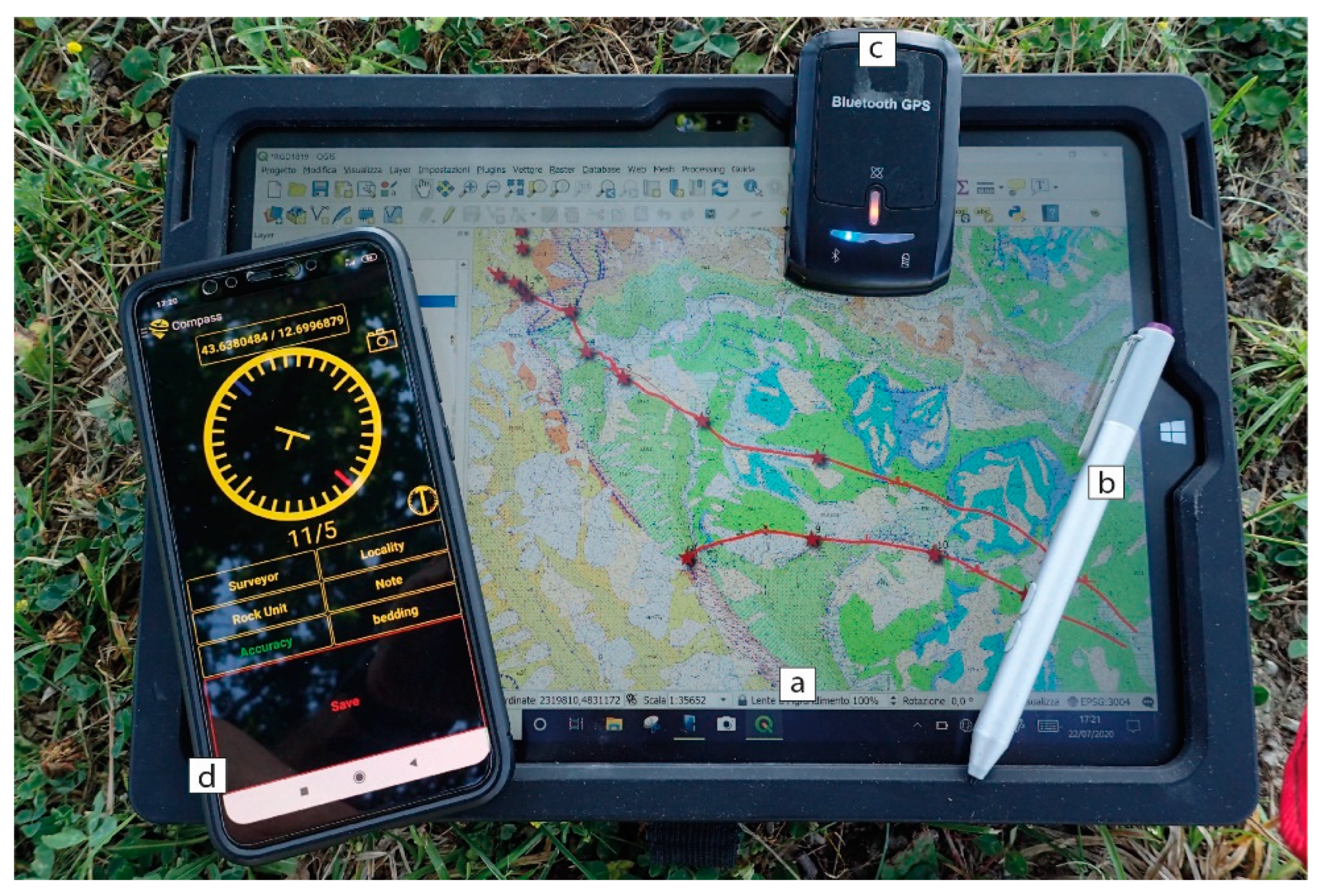
2.1. Digital Field Mapping

Geologists are used to working with a pen-on-paper system; therefore, we wanted to adopt and modernize this useful habit by switching paper to a screen and changing the pen/pencil to a digital stylus. The hardware equipment used for the ground survey were: (i) a tablet PC (Surface 3 Pro, OS Windows 10; Figure 4a) with a stylus as an input device (Figure 4b) and a built-in camera (the tablet PC was ruggedized using a plastic and rubber cover with wrist ergonomic support); (ii) a small 51-channel Bluetooth GPS receiver and an SIRF antenna with the NMEA protocol and EGNOS correction (Figure 4c); and (iii) an Android smartphone with built-in GPS and a camera (Figure 4d).

The software tools used were: (i) QGIS 3 [35], an open-source GIS software, coupled with a full set of geological plug-ins, such as BeePen [36] for rapid annotation, BeePic for picture georeferencing, BeeJou for Windows Journal file georeferencing, BeeDip [37] for direct import/export of structural data from the homonym Android app, DirectionalSlope [38] to perform morphology analysis on DEM, and qgSurf [39,40] to calculate the fault plane/DEM intersection; (ii) Windows Journal as a field book for taking notes and sketching; and (iii) the BeeDip Android app for collecting structural georeferenced orientation data (i.e., bed dip, fault surface, and lineation measurements) and oriented pictures.

The ground field work was done in a similar way as the pen-on-paper method using the stylus on the screen of the tablet. We used many raster base maps of the Marche region at the scale of 1:10,000, such as topographic [41] and geologic maps [42], as well as aerial orthorectified images organized in layers. Some vector layers were prepared for collecting data such as bedding measurements, fault geometry, and kinematic data on outcrops. We also assembled some input data using Qt Designer [43]. Moreover, we collected information in the same way as a field book using Windows Journal (free software for Windows) [44] by writing down notes and drawing sketches. Other layers were added for elaborations of fault system traces, geological units, etc., that allow drawing of the geological maps.

2.2. UAV (Unnamed Aerial Vehicle) Survey

The aerial survey was carried out using DJI Inspire 1 v2.0 [45] equipped with a 12-megapixel camera (CMOS Sony Exmor 1/2.3 sensor), which is able to capture clear and bright pictures (Figure 5a). The geometry drone frame provides good wind resistance, an important characteristic in mountainous areas. The flights were planned and controlled using two different software products: (i) UgCS [46] with the function of keeping the drone at the same altitude above the ground during the flight, pre-loading a DEM or using Google Earth [47] (Figure 5b) and (ii) PiX4D [48], mainly used for vertical surveys and allows to pre-set horizontal and vertical shooting positions (Figure 5c).

The photographs (20 gigabytes) captured during the survey were subsequently processed with Agisoft Metashape [49] (Figure 5d). This software allows the creation of three-dimensional (3D) virtual outcrops starting from a photo sequence taken with an 80% overlap. The processes consist of importing images, aligning photos (after recognizing the same ground points), creating a dense cloud, creating a mesh, and adding texture to the mesh. Therefore, we obtained a DEM wrapped by georeferenced photos to create a virtual outcrop.

2.3. Three Dimensional Modeling

We also imported the drone survey DEM into Rhinoceros [50] in a digital terrain model, where we could draw the mapped fault trace and then visualize the 3D fault plane.

Data from the maps, sections, and point clouds (from the drone survey) were collected using Move software [51] and a detailed 3D model was designed for the studied area. This model was then applied to a larger section of the Umbria–Marche Apennines to define the possible relationships between crustal structures.

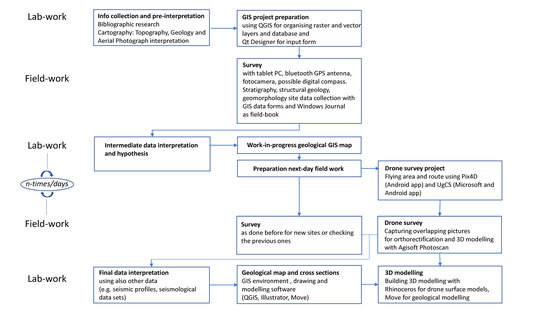
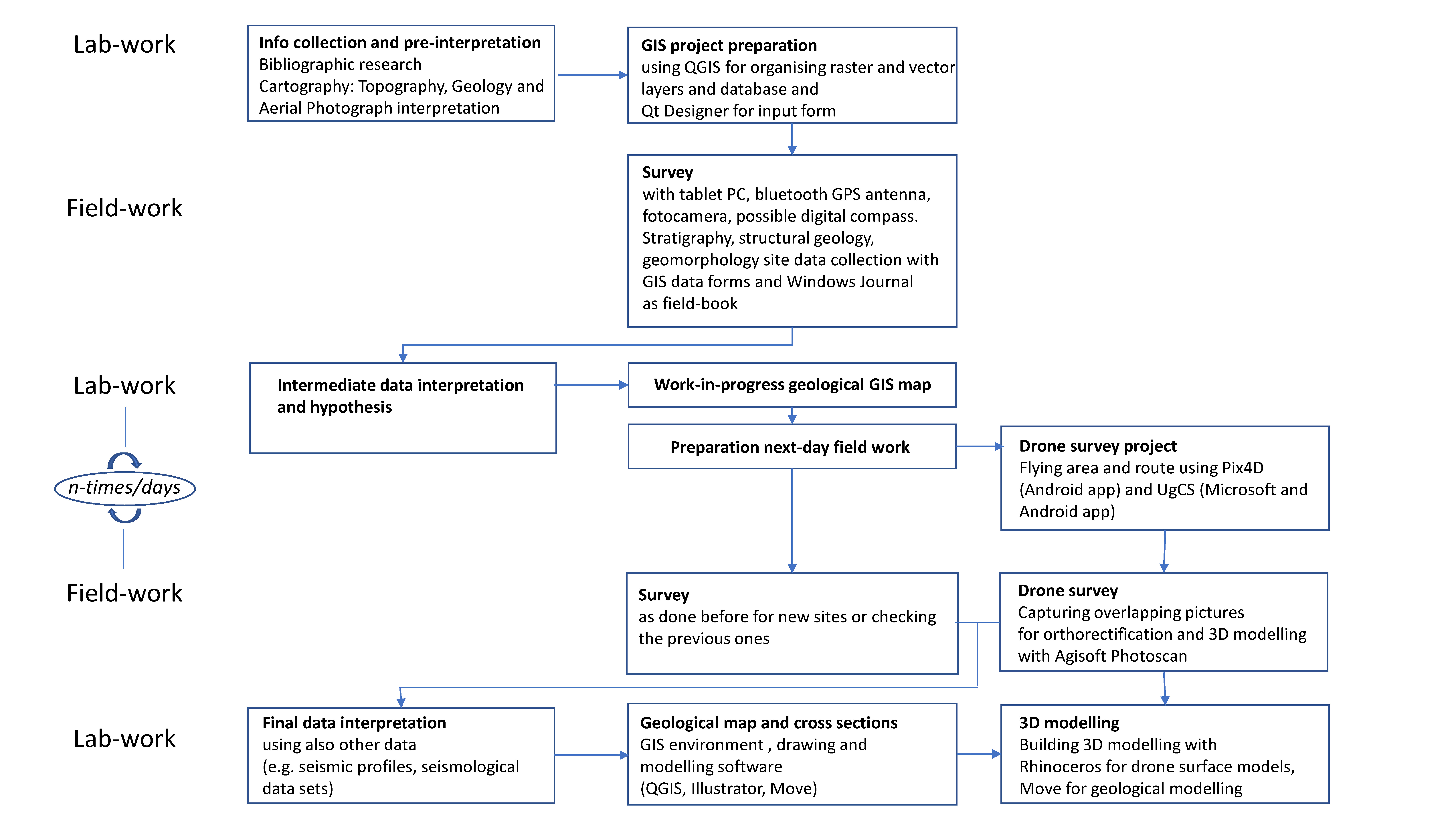
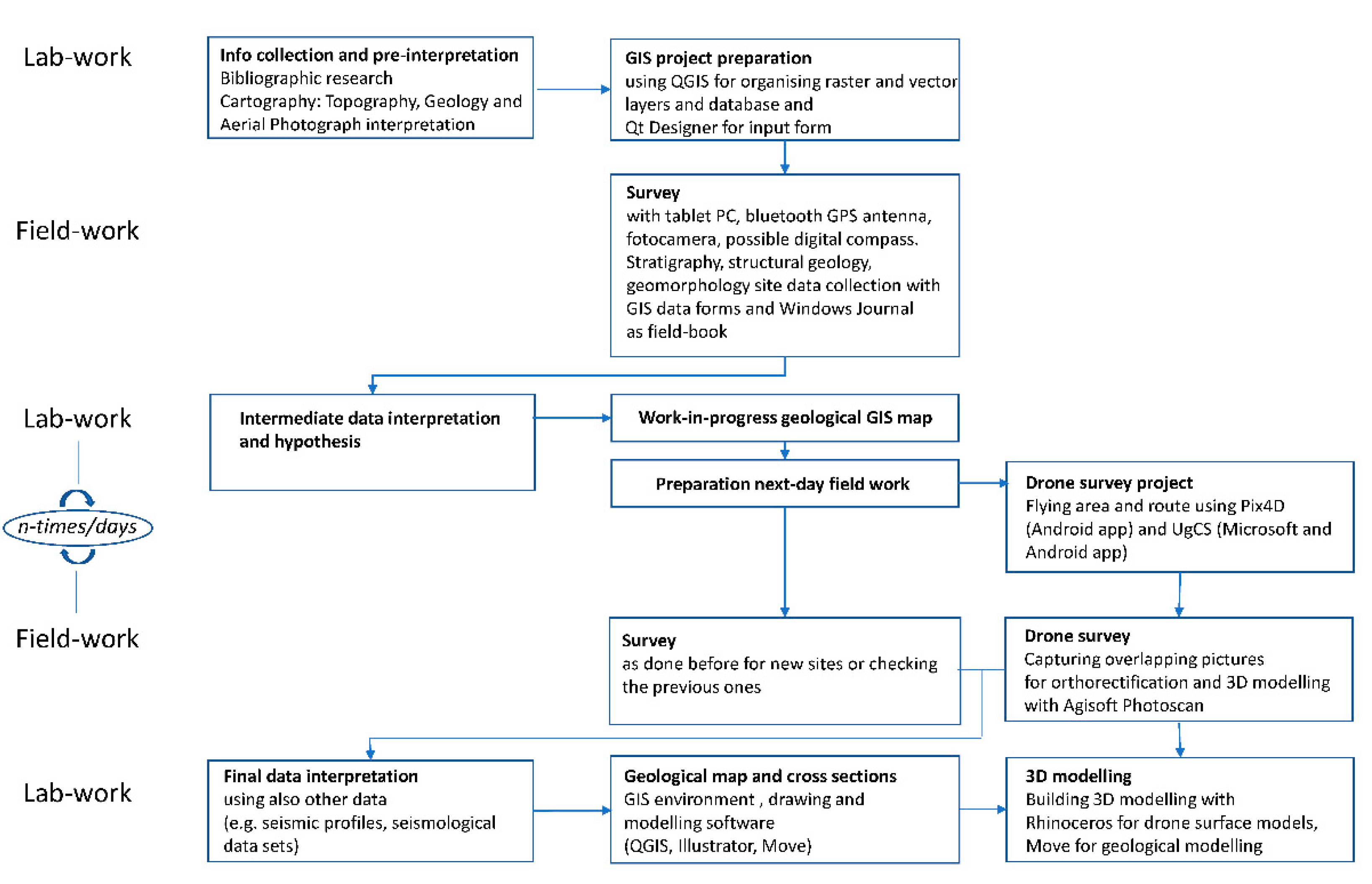
3. Methods and Workflow

The traditional mapping method of using paper maps involves several “indoor” and “outdoor” steps to be carried out properly. We wanted the digital mapping method described in this article to follow the same steps in terms of changing tools and needing more digital knowledge. For this reason, we proposed a workflow (Figure 3) that allows defining the various phases (repetitively in some cases) of digital work, both in the field and in the laboratory.

3.1. Laboratory Work

Before performing field work, the campaign needed to be carefully planned. To start, bibliography and cartography research was carried out, and all relevant papers that included our study area or were of a similar topic were read. Moreover, maps of different cartographic styles were collected:

• Topographic maps, in this case, the Marche region technical map (C.T.R) [41] at the scale of 1:10,000. This map is quite new and detailed, and is available in GeoTIFF format (georeferenced raster format) [52];
• Geological maps from the same agency (Marche region geological map at the 1:10,000 scale) [53], which distribute raster (GeoTIFF) and vector (Shapefile format) formats at the same scale as the C.T.R.;
• Scanned and georeferenced raster maps of recent aerial photographs.

These data, together with the study of aerial photos and landscape shapes (topography and DTM), were very useful for a first interpretation of the lineations that could pertain to a system of recent faults.

In addition to the visual interpretation of aerial photos and topographic maps, we used tools such as the QGIS DirectionalSlope plug-in [38] to consolidate the first interpretations with a morphological analysis tool, also using a DEM at 20 m [54].

Once the data and maps were collected, a GIS project was created with layers for all the different maps. To be able to read this amalgamation better, the white background was replaced by a transparent one (i.e., in the C.T.R.). Furthermore, the following new vector layers were created for data and note collection:

• Bed attitudes (points)—for dip data collected in the field;
• Fault data (points)—measurements on the fault surfaces, kinematic indicators, etc.;
• Outcrops (polygons)—for drawing geological units, facies, or guide layers;
• Annotation faults (lines)—for drawing tectonic lineaments;
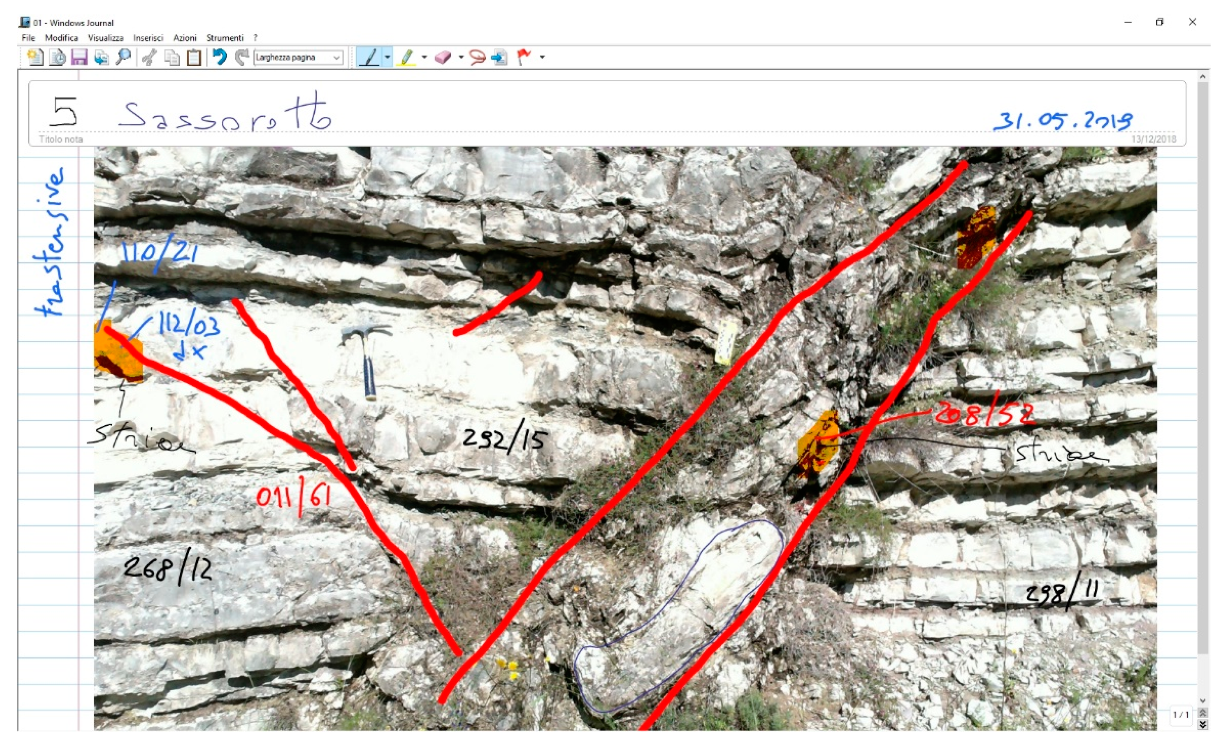
• Field book (points)—for entering information collected in the “field book” using Windows Journal [44].

To make it easier to collect data in the field, input forms were created using Qt Designer [43] and linked to the GIS layers (Figure 6a). After this process, the next step could be conducted, i.e., the field survey, taking into consideration that any part of the project could be changed or improved at any time.

3.2. Field Work

This step was carried out in collaboration with postgraduate students during their digital survey field camp, which lasted a week. All data were collected using a tablet PC, to which a small GPS antenna was connected via Bluetooth (Figure 4c). Using these tools, data were collected to (i) improve the geological cartography already available (e.g., detailing the stratigraphy of the terrigenous lithofacies); (ii) check the spatial arrangement of the faults interpreted in the laboratory; and (iii) collect new data on outcropping faults.

The pre-set data entry form for storing “structured” data (Figure 6a) and the Windows Journal digital “field book” that allowed us to write with the stylus on the screen were fundamental to frame the hypotheses (i.e., models and schematic sections) and to sketch outcrops (Figure 6b). In this application, cameras (integrated in the tablet and personal camera) proved to be very useful to capture and import photos to the Windows Journal page, allowing us to draw and write notes.

The QGIS plug-ins created in the lab were very useful. BeePen allowed us to quickly write notes and to draw (e.g., fault traces) with the stylus on the screen in the same way as the classic method, i.e., pen-on-paper (Figure 6c).

A new app, namely, BeeDip (Figure 6d), which is still under development, was tested for the gathering and georeferencing of structural data (i.e., surfaces and lineations). This app has an open-source license for smartphones with an Android operating system. Here, the geological map was imported from the GIS project, and the map was split into tiles for daily work. Dip and lineation data were then imported into the GIS project, as well as the georeferenced photos. Export from and import into the GIS project were possible, thanks to the GeoPackage interchange file format (.gpkg) that allows management in a SQLite database of the vector features, tile matrix sets of imagery, and raster maps at various scales and with various attributes (non-spatial data) and extensions [55].

3.3. Intermediate Laboratory Work

Every evening, after field work, the data were analyzed to formulate new working hypotheses and to organize field work for the next day. This intermediate phase was repeated with the students throughout the field camp and subsequently during individual work.

In this phase, the data collected by the working groups of students were validated and merged into one common GIS project. This step improved the interpretation using a new summary geological map, which made it possible to almost immediately review the initial interpretation of the fault traces on the topography, as well as to update strategies and methods of data collection. Sometimes, data entry forms were revised and corrected based on the needs that arose during the field work.

The information collected in panoramic photos is very useful, even when taken remotely in inaccessible areas. That was why, we started using drones in our data collection procedure. This was possible, thanks to two of the students who had a drone pilot license and training in aero-photogrammetry. Various software applications were used to prepare the flight plans. In particular, UgCS [46] software was very useful, since it allows planning of flights that follow irregular mountain topography. The flights, with swipes and times, were planned on a laptop (Windows operative system) and exported to the homonymous app on the Android smartphone to be used to conduct the field work.

3.4. Continuing the Field Work

The intermediate phases of field and indoor work led to improvements in the interpretation and working method, and to the identification of other measuring stations along the fault traces. Any sites for which the interpretation was uncertain or data were not sufficient or convincing were re-checked. During these days, several aero-photogrammetric shooting missions using drones were completed, both by using the pre-set flight plans and by flying “freehand” in areas where it was still difficult to shoot important details (e.g., nickpoints inside creeks).

3.5. Final Laboratory Data Elaboration and Interpretation

The alternating field/laboratory work method resulted in a final map and reasonable interpretation of the investigated faults. The DTM and the ortho-photographic reconstruction of flights using Agisoft Metashape (Figure 5d) contributed to the final interpretation, through the structure-from-motion algorithm (SfM) [56,57,58,59]. The outputs were then imported into GIS and visualized in Rhinoceros, where some portions of the faults were drawn on surfaces in a 3D environment (Figure 7).

The final interpretation included other data, such as seismic lines [60] and data from the National Institute of Geophysics and Vulcanology (INGV) earthquake catalog [61]. In this way, in addition to the GIS geological map, it was possible to create a 3D geological model and cross-sections with Move software [51]. This suite allowed us to integrate and visualize all of our data for a more comprehensive understanding.

4. Examples of the Laboratory Preparation, Field Mapping, and Final Interpretation Work

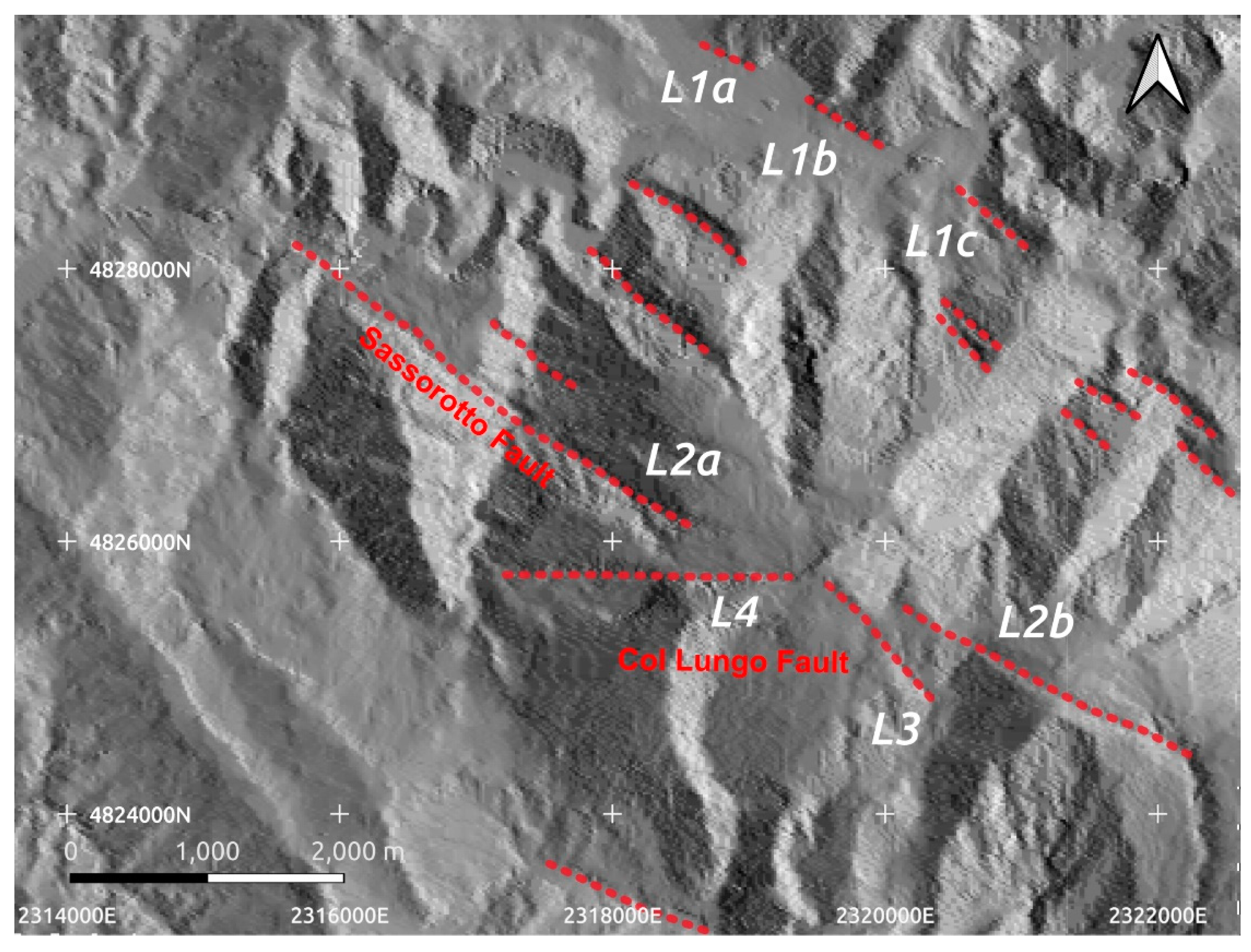
4.1. Initial Laboratory Work: Morphological Lineament Analysis

In order to supplement the cartographic information with topography-derived lineament orientations, we performed a set of analyses on the directional slopes as derived from a 20-m resolution DEM. The analyses were performed in QGIS using the DirectionalSlope plug-in. The directional range was from 0° to 350°, in increments of 10°. Obviously, the 180°–350° maps inversely mirrored the 0°–170° maps.

A visual assessment of the potential lineaments was performed, and the most interesting map was considered as the one related to the N080° orientation, highlighting the lineaments with a NW–SE orientation. The potential lineaments were manually digitized when related to the anticlinorium structure, avoiding as much as possible, in this first phase, the influence of other types of information (i.e., geological maps and remote sensing images). The results are presented in Figure 8, with the majority of mapped lineaments showing a WNW–ESE trend, with the exception of one E–W lineament (L4) and one NW–SE lineament to the south of Monte Nerone (L3).

Near the northeastern margin of the mapped zone was a set of three aligned lineaments (L1a–c in Figure 8), separated by alluvial sediments, that possibly constituted an unmapped, single ENE–WSW normal fault which occurred along the northern boundary of a small basin. If so, the mapped fault extended at least 3 km. Other lineaments with the same orientation occurred in the northern part of the mapped area, but had limited longitudinal extents of approximately 1 km or less. They corresponded to abrupt lithological changes of stratigraphic or possibly tectonic nature and were not mapped as faults.

A more prominent lineament (L2a; 3.6 km) was almost aligned with another one (L2b; 2.4 km), while being separated by a 1.6-km gap. Interestingly, the L2a segment ended where a mapped E–W fault might offset this segment. The L2b segment was also mapped as an undefined lineament in the geological map. Another developed lineament was an E–W lineament in the center of the mapped area (L4), with a longitudinal extent of 2 km.

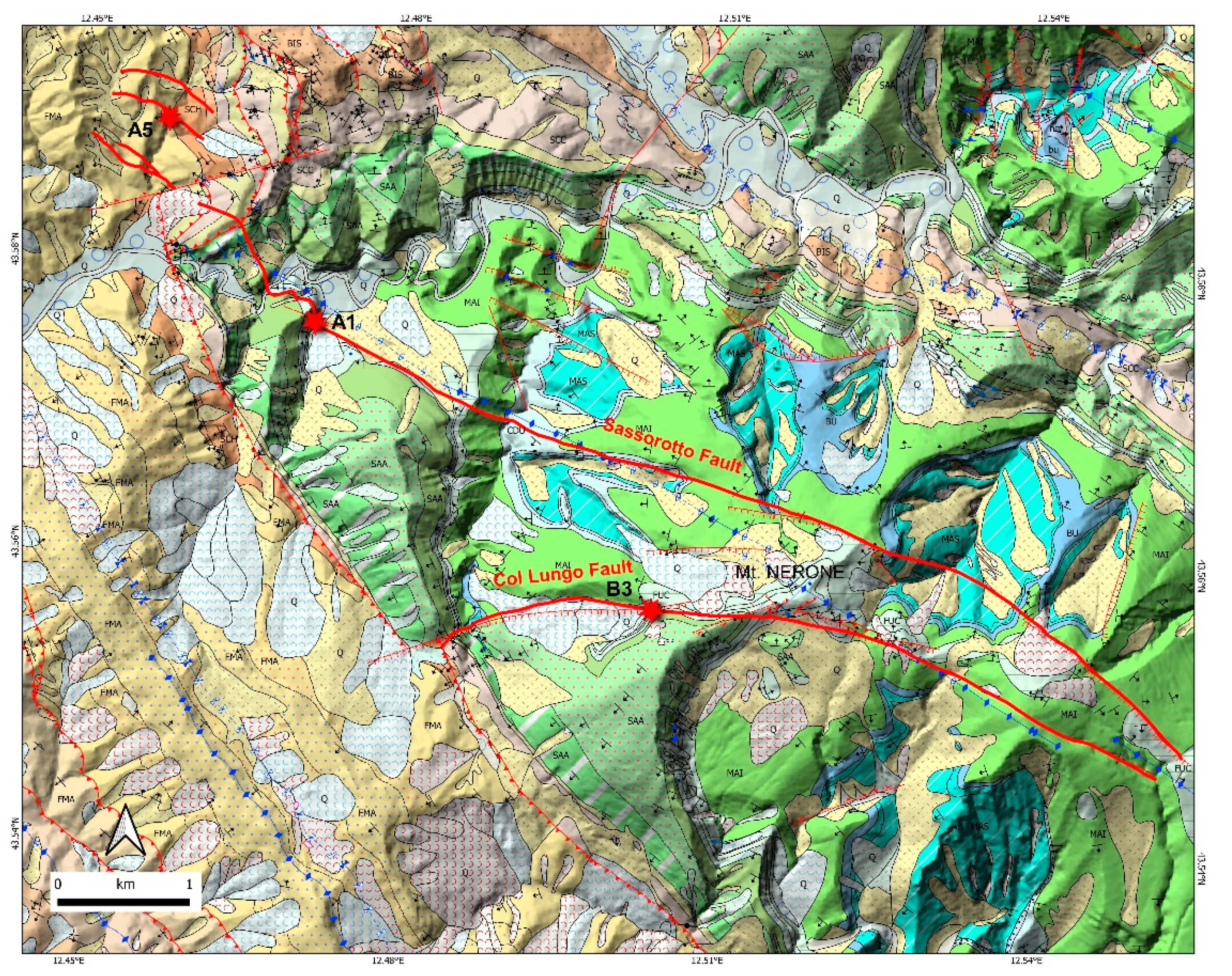
4.2. Field Work: Survey and Measurement Sites

The geological survey was carried out after interpretation and analysis of the aerial imagery and maps. We chose some measurement sites (Figure 2), where we collected data on the outcrops along the alignment of the interpreted fault trace. Two main faults were mapped (Figure 2), showing that even the fault system could be more complex.

• Sassorotto fault: The main fault cutting the crest of Monte Nerone and continuing SE (even if less evident); toward the NW, it reaches the Biscubio valley and continues toward Monte Vicino, affecting the Miocene terrigenous turbidites of the Marnoso Arenacea Formation.
• Col Lungo fault: A minor fault that shows important evidence of recent extensional activity from La Valle Agriturist, through the Col Lungo escarpment, to the road at the top of Monte Nerone and continuing with further morphological evidence to La Montagnola and beyond, toward the SE.

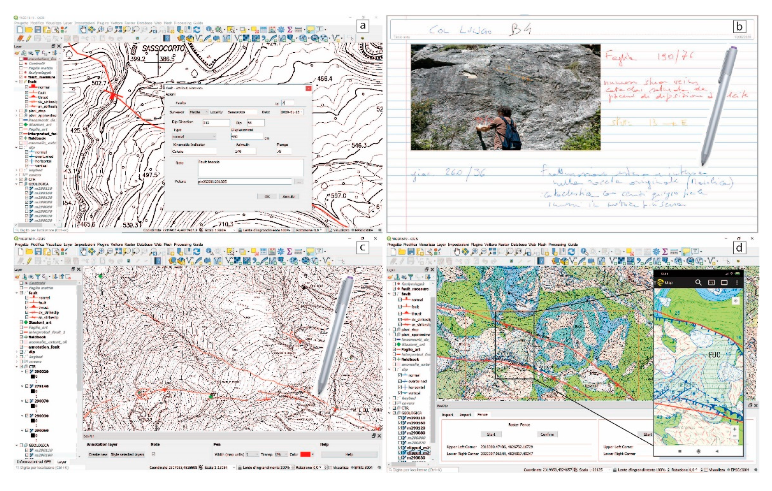
4.2.1. Site A1—Sassorotto (Field Mapping)

This site, which the fault was named after, is located quite close to the main Apecchiese road and it is easy to access. A continuous outcrop of the Scaglia Bianca Formation is well-exposed along a historical and almost forsaken path beyond a closed barrier. The fault shows a brecciated zone that is half a meter thick, with surface dipping to the SW. Some other conjugate minor antithetic and synthetic faults can be observed (Figure 9). The stratigraphic succession could indicate that the movement is normal, but it does not allow measurement of the actual displacement, which is not less than 4 m.

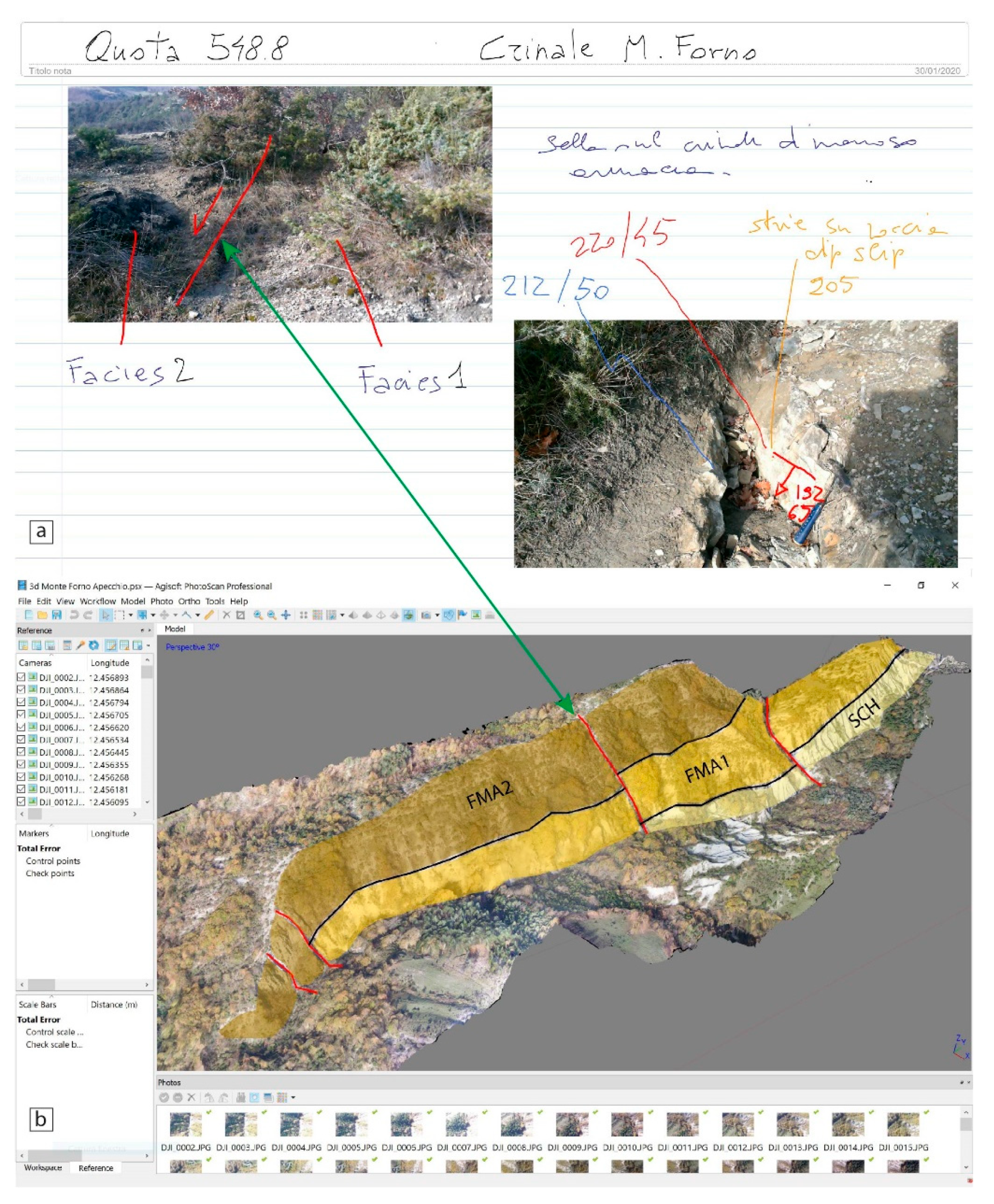
4.2.2. Site A5—Monte Forno (Field Mapping)

Along the stream near the small village of Monte Forno, the outcrops show Miocene terrigenous deposits starting (bottom to top) with the Schlier (SCH) Formation and continuing with the turbidites of Marnoso Arenacea (FMA) with a typical thickening upward succession. The fault traces are more rambling because of the mechanical response of these marly sediments. Three main normal faults dipping to the SW can be mapped. These quite recent faults cut a very incised valley and some step along the stream bed.

Here, the survey was carried out using all of the available tools. Following field mapping with the tablet, GPS, and mobile GIS (Figure 10a), the drone flight captured georeferenced pictures for the following orthorectification and more detailed georeferenced DTM. This also allowed for a more detailed 3D interpretation and mapping (Figure 10b).

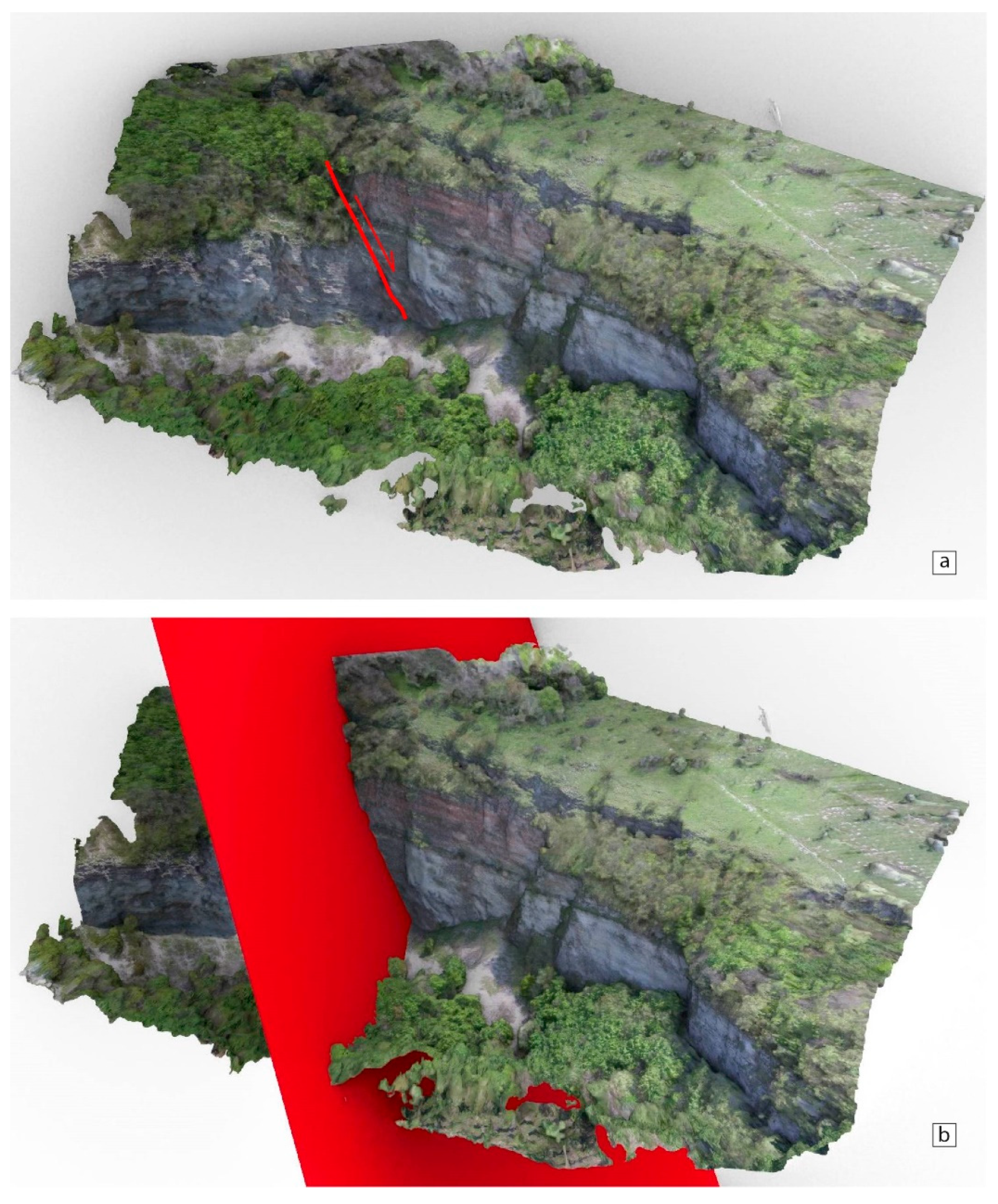
4.2.3. Site B3—Col Lungo (UAV Survey)

This large outcrop is visible from the road, descending from the top of Monte Nerone to the village of Serravalle. It is located at a site difficult to reach in some parts. Moreover, a large part of the outcropping succession is dissected and the cliffs are very close to falling down, posing notable risks for surveyors. Under these circumstances, the UAV flight was helpful for capturing the fault outcropping in the northern sector of the outcrop, where the Maiolica Formation constitutes the footwall of the fault and the Scaglia Bianca and Scaglia Rossa formations are on the hanging wall.

The drone photos were combined into a DTM, from which a 3D fault surface was built to obtain orientation data (Figure 7).

4.3. Intermediate Laboratory Work: Analyses of Fault Attitudes

We attempted to check a possible interconnection between the main faults in the central part of the studied region by using a Python plug-in in QGIS for the delineation of planar surface intersections with DEMs, namely, the plane–DEM intersection module of the qgSurf plug-in [39,40]. This plug-in calculates the intersecting points between a plane defined by its dip direction and plunge using the provided DEM.

By means of trial-and-error, we found a mean plane attitude that fit quite well with the tentative fault segments, as mapped in the Marche region geological map (Figure 11). It honored the A1 location, neared the A3 stop, and approximated quite well the mapped fault segments in the geological map.

The mean plane had a dip direction of 205° and a plunge of 55°, not that dissimilar to the fault plane measured at the A3 stop (212°/38°). In the case of fault B, we had to use two slightly different attitudes: one with an attitude of 173°/55° in the western sector (B4–B5 segments), while for the more developed eastern section, a better fit was provided by an attitude of 196°/47°.

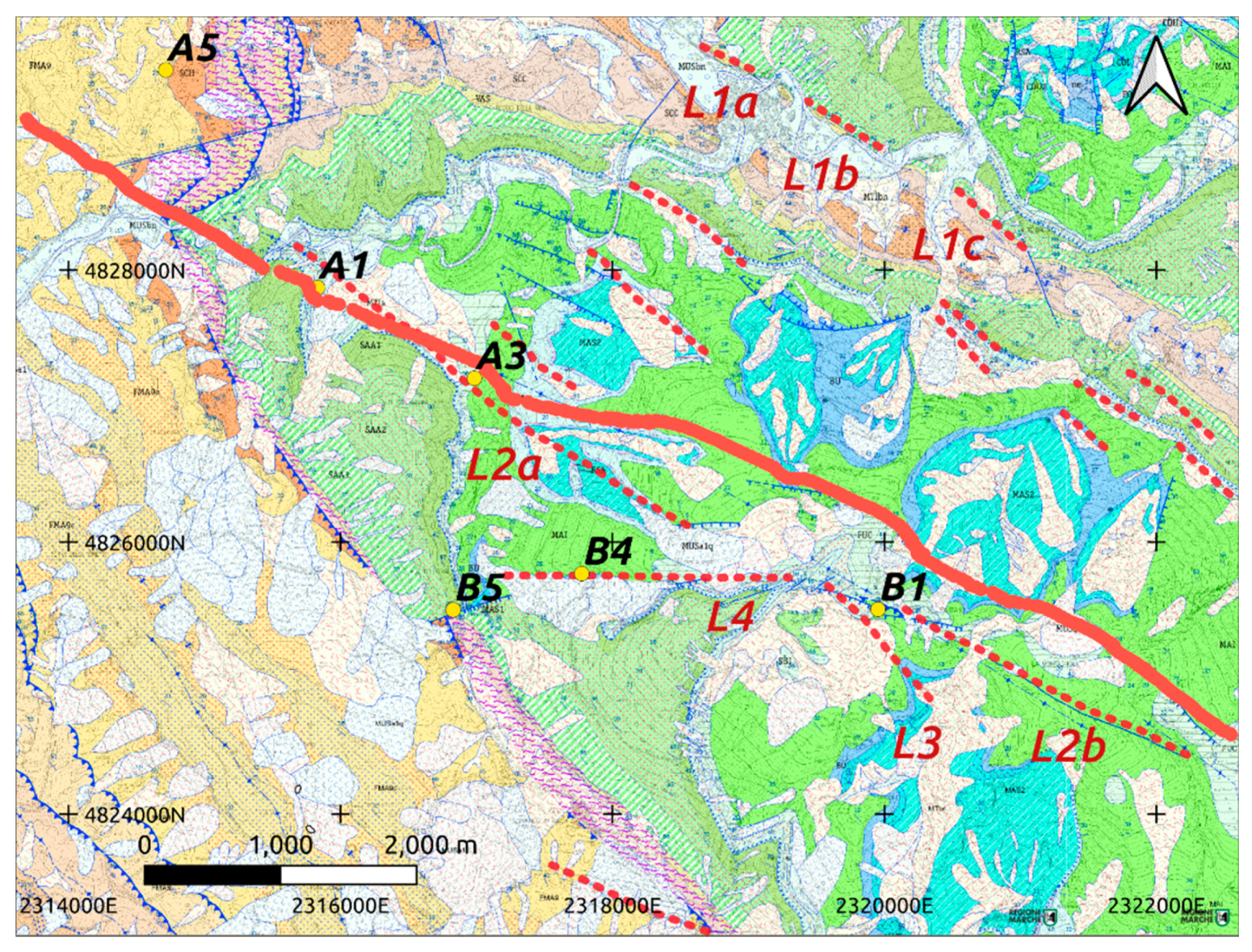
5. GIS Elaboration of the Geological Map

The data collected digitally within the GIS project led to the creation of a new (possibly seismogenic) fault map (Figure 2), in which faults related to an extensional system were reported for the first time. The local elements of these faults were already mapped in the last geological regional map (scale 1:10,000), but they were not interpreted as a system cutting the ridge, the whole Monte Nerone NW flank, also extending toward the terrestrial syntectonic deposits of the Marnoso Arenacea or Sandstone of Monte Vicino formations [62].

The subdivision into facies easily recognizable in the ditch of the Monte Forno outcrops (Figure 10b) made possible a first interpretation of the faults, even though the fault surfaces were not visible. In detail, from bottom to top, the three facies are: Pelitic facies without arenitic levels (Schlier Formation), whose contact with the oldest formations of the Scaglie Group is tectonized; pelitic facies with thin arenitic levels (Marnoso Arenacea; FMA1 in Figure 10b); pelitic–arenitic facies with medium and thick arenitic levels (Monte Vicino Sandstones; FMA2 in Figure 10b). Moreover, the analysis of the DTM allowed for the identification of uneven morphology with abrupt non-eroded counter-slopes even along the ridge, this leading to the hypothesis of very recent morphogenesis.

6. Combining Other Data

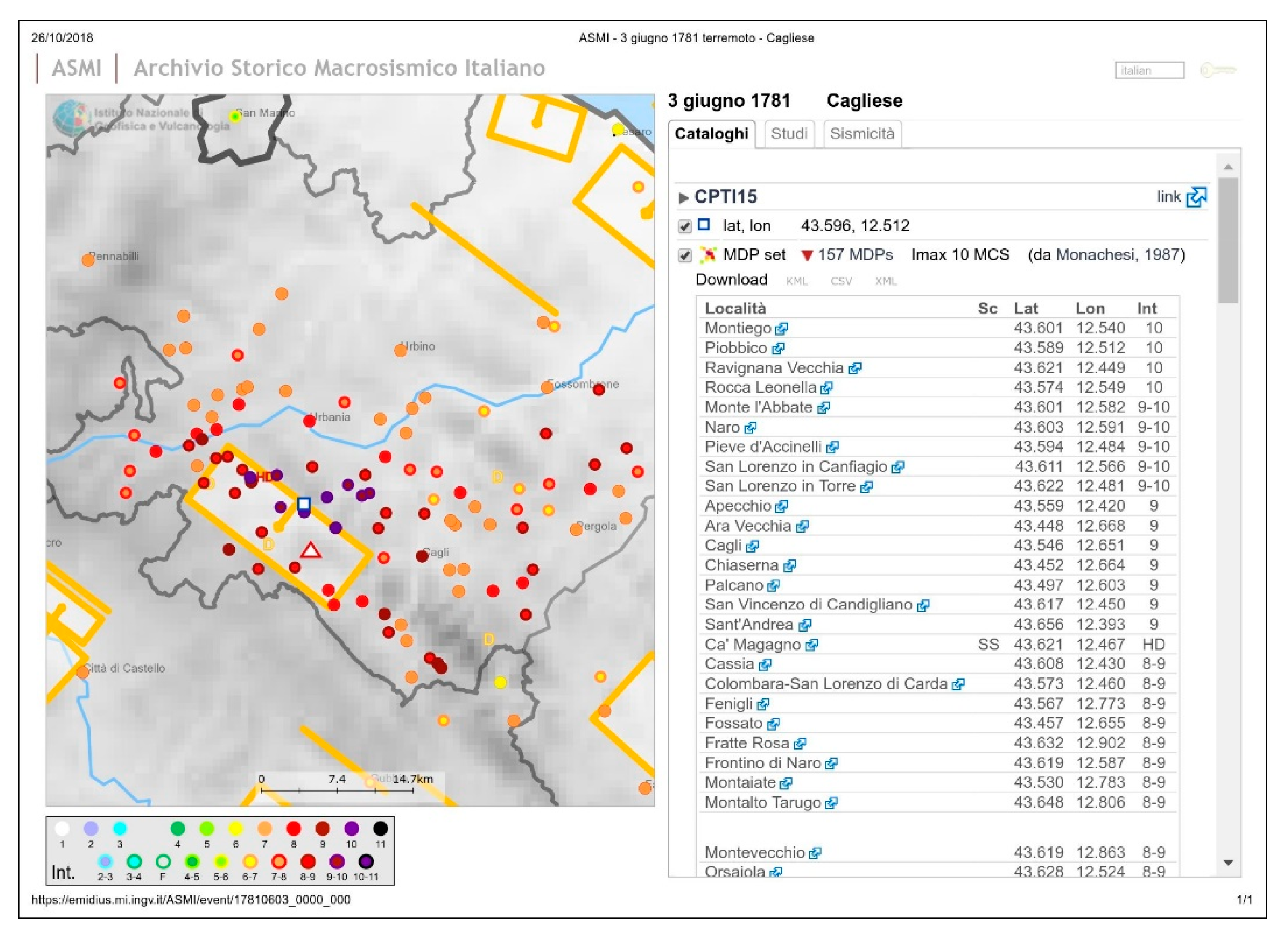
6.1. Historical Seismicity

Research was carried out by integrating the available data in the INGV catalog with those of the Italian Historical Macroseismic Archive [63] and the Parametric Catalogue of Italian Earthquakes [64,65].

Among the historical events of the area between Umbria, Marche, Tuscany, and Romagna are some well-known events, such as the 1781 Cagli earthquake [12,13] and others of less reliable sources but reported in catalogs [66], such as the event on 17 April 1725 in the Monte Cardamagna area, according to the chronicles of the time. These events, although with uncertain locations and intensities, constitute an important indicator of the historical seismic activity of the area (Figure 12).

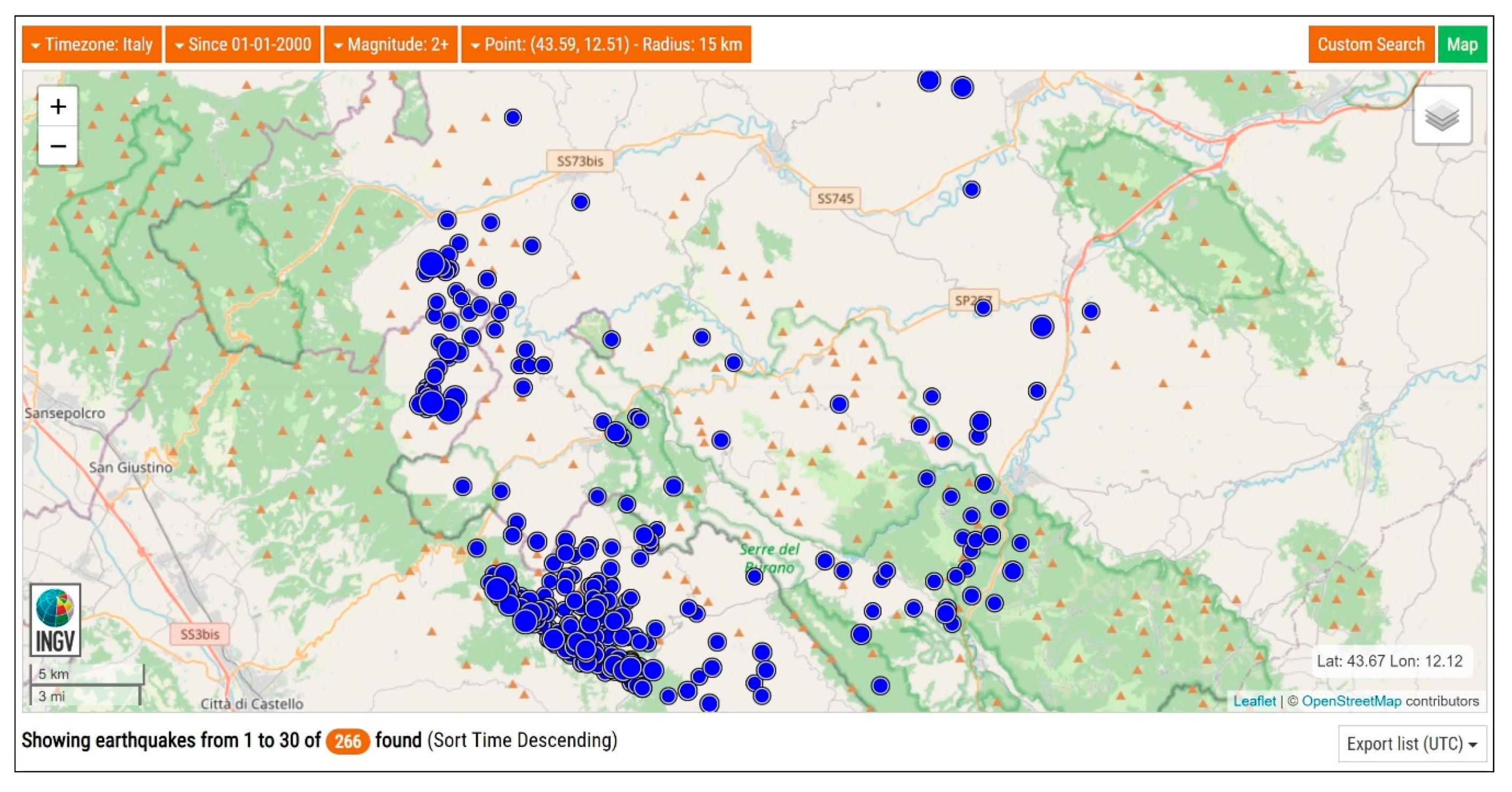
6.2. Instrumental Seismicity

The very recent seismicity instrumentally recorded in this area provided a large dataset that helped to define the geometry of the structures at depth.

On the INGV website (ISIDe Working Group, 2007) [61], it is possible to query and download information in various formats on earthquakes that have occurred worldwide, almost in real time. The parameters provided are: the location of the hypocenter (geographical coordinates in the WGS84 system and depth in kilometers above sea level), the estimated Richter magnitude (local magnitude (ML) for earthquakes with M > 2.0 and, if possible, the moment magnitude (Mw)), and the time of origin (date and time in the Italian and Coordinated Universal Time (UTC) time zones).

Through a customized search, seismic events were identified that occurred at any depth, within 15 km of Piobbico, and during the last 20 years (Figure 13). This dataset was downloaded in text format and imported into the Move work environment and visualized as a cloud of points, where each point represented a single event, geolocated in depth.

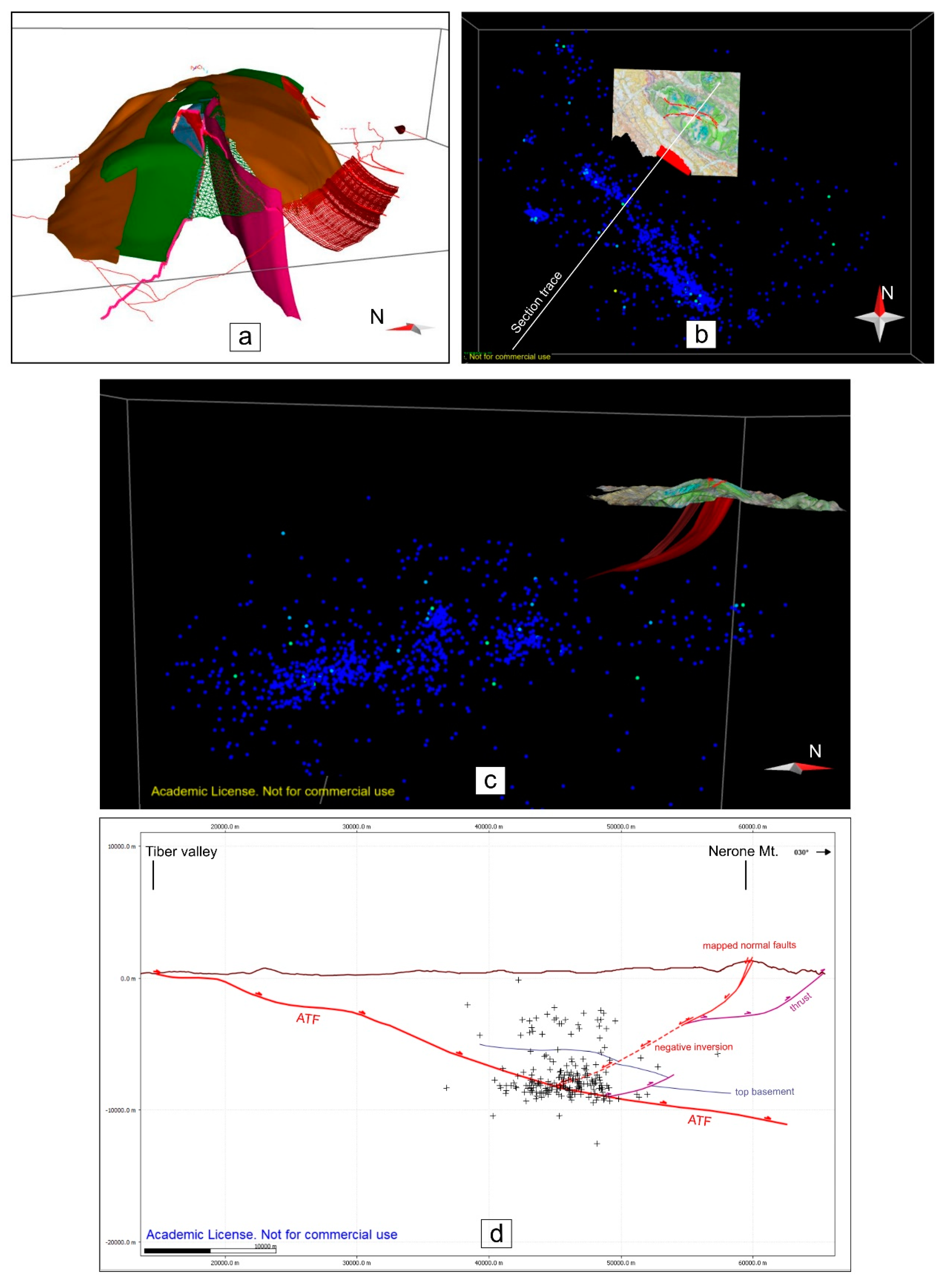
7. Three Dimensional Modeling

The geological map with traces of the interpreted fault surfaces was imported into the Move three-dimensional environment. Here, the first 3D geological model was built using the cartographic and new field data (Figure 14a) with well-known procedures [67,68,69]. This model was then improved with the information from the new DTM derived from the drone flight. In particular, in some areas (i.e., Sassorotto, Monte Forno, and Col Lungo) from the DTMs built with Rhinoceros, it was possible to extrapolate the surfaces of the faults in three dimensions (Figure 7).

The model of this sector of Monte Nerone and the surrounding areas made it possible to reinterpret the relationships and offsets of the faults, even at shallow depth (approximately 1 km). Additionally, the integration with the available commercial seismic sections and CROP 03 (see Figure 1) [18] allowed us to extend the model in depth, thus improving the interpretation of the relationships between the studied faults and other well-known regional faults, such as the Alto Tiberina fault (ATF in Figure 1) [25,70].

To support our hypotheses, the hypocenters of instrumental and historical earthquakes were added to the three-dimensional model (Figure 14b,c) and into a regional geological section (Figure 14d).

8. Results and Discussion

New results for geological investigation and interpretation, the importance of which lies in the possibility of identifying very recent and capable structures, will be discussed below.

However, as already expressed, the aim of this work was to define a workflow, adaptable even to other geological and territorial contexts. Therefore, we will discuss in depth the results on the detection, cartography, and modeling methods that can be applied in similar situations and for similar purposes.

8.1. Geological Results

• This study and the data collected led to a different interpretation than that reported in the literature (e.g., [20,71]). The results indeed highlighted the presence of a system of recent normal faults with respect to thrust and fold structures. The Sassorotto and Col Lungo faults showed irrefutable stratigraphic and structural evidence of extension. This system of shallow faults is very similar to those detected and mapped in the areas of the earthquakes in central Italy in 2009 and 2016 [5,72,73,74].
• Surface and deep reflection seismic data (CROP 03; [18,75]) crossing the mountain belt very close to the study area and the distribution of the epicenters [61] provide indications similar to those reported by various authors [3,27,28,29,76,77,78,79] for the southernmost areas shaken by recent earthquakes. In our case, the evidence of normal faulting on the surface could be related to deep stretching, with negative inversion of thrusts, as demonstrated in areas further south [80,81,82,83]. The interpretation that places the extensional regime now east of the Apennines watershed, toward the Adriatic, is also supported by evidence reported by several authors in neighboring areas [21,22,23,84,85].

In the study area, the extensional tectonics are also highlighted by geomorphological evidence, such as anomalies of the hydrographic network [86,87], inversion of the relief [88] and “young” complex ridges with counterslopes, and breakages of the slope itself. Although still in a preliminary phase of study, the collected data suggested a very recent, certainly Quaternary age faulting.

If so, the mapped faults might be capable of large earthquakes, and therefore, may be the source of the 1781 Cagli earthquake centered in this region. This system of faults can be considered capable, as defined by the Italian National Institute for Environmental Protection and Research (ISPRA) [89] and the International Atomic Energy Agency (IAEA) [90,91].

8.2. Methodological Results

• The availability of inexpensive and now very popular tools allows everyone to work “digitally” in the field. Until a few years ago, tools such as tablet PCs were much more expensive [92], and their characteristics were somewhat limiting (performance, light readability, weight, etc.). For this study, normal tablet PCs (not ruggedized) were used, since the working conditions on the ground were not adverse (e.g., no rain or dust) and the covers used kept them safe from small falls. A normal tablet costs 4–5 times less than that of a ruggedized one and has a lower weight making it easier to carry in the field.
• The use of an external GPS receiver is a limitation, but only if the tablet and receiver are carried by different people. In this case, the Bluetooth connection could become disconnected and the software would thus not receive the necessary signal. To avoid this problem, a small pocket receiver weighing less than 100 g could be used to receive signals from different satellite constellations. Here, we used a cheap 51-channel receiver, which performs with high cartographic accuracy.
• The drones used were all common and affordable, capable of adequate flight times and extendable working times with additional batteries, and light weight to improve the transport possibilities. Drone operation is controlled by country laws and regulations that evolve fairly quickly in the attempt to adapt to technological innovations. Currently, in Italy, it is possible to use a drone with weight less than 300 g without particular restrictions. The drones we used were driven by students with a valid flight license and with the appropriate insurance, even if the areas flown over were mostly or completely uninhabited. Since drone flights allow the possibility to take very accurate photogrammetric images and extremely detailed DEM, such a digital survey method is an instrument of great potential.
• The integrated terrestrial and airborne digital survey systems enabled us to collect data from different observation points, a very important fact in the context of geological observations where it is important to switch from macro- to micro-scale and to different angles. The gathered data were organized on digital platforms as they were collected. This strategy provides some advantages such as the elimination of mistakes related to transcription and changes of scale [93]. An example is the case of the survey in the Monte Forno area, where the interpretative synthesis of both stratigraphy and tectonics was improved. The observations and mapping of the outcropping lithofacies enabled a first interpretation, even if the fault planes were not visible.

The survey along the ridge on the right hydrographic was managed with a tablet PC and a compass, even if the meaning of the data was not immediately clear (e.g., lateral changes of lithofacies). With the drone panoramic images, it was possible to determine that these lateral changes could be related to faults that displaced the hanging wall to the SW. The detailed DTM created with the drone pictures made it possible to highlight along the ridge along an uneven morphology, with abrupt counterslopes along the fault planes. In an inaccessible riverbed, this DTM also highlighted the presence of small waterfalls and nickpoints, exactly in correspondence with the interpreted faults. Therefore, it is possible to hypothesize very recent morphogenesis related to recent tectonic activity.

• The chance to work both in the field and in the laboratory with a single GIS software, such as QGIS desktop [35], without switching between different software and formats, is an advantage in terms of the time and the risk of introducing errors.
• To carry out a digital survey, appropriate tools are required that are suitable for field work. Here, new tools were created to be integrated with QGIS. The plug-ins described in the previous chapter were derived from the need for an easy method that is compatible with GIS, and that is also close to the traditional method of field work, i.e., pencils and paper maps. BeePen [36] and BeeJou, tools for quickly taking notes and georeferencing Windows Journal files, were conceived and created to take advantage of stylus and ink technology [94]. Moreover, the idea of a digital compass interacting directly and simply with the QGIS software led to the development (now at an advanced stage) of BeeDip [37], which is both an Android app for collecting structural data and a plug-in that allows the input and output exchange of data and maps between QGIS and the smartphone compass.
• The flexibility of the system in the organization of collected data allows changes/additions during the work. This becomes useful when new hypotheses are developed, when the area is not well-known, or when working in teams of geologists with different experiences and skills. In our case, this flexibility allowed to rearrange the project, using models that evolved during the work, contributing to the final synthesis. This feature, combined with the possibility of storing ideas, hypotheses, and validations in a temporal sequence, allows georeferencing of the analytical and deductive thinking that the geologist makes during field work and in the laboratory.
• The availability of well-organized digital data (tables, sheets, geolocation, etc.) allows a simpler, faster, and more correct import into cartographic and multidimensional modeling software. In addition to the classic geological maps, this method allows a more comprehensible overall synthesis, together with validation of the conclusions. In fact, in a three-dimensional model, for example, the shape and position of the fault tip lines must be defined as much as possible, while on geological maps they often end with uncertain dashed lines. Furthermore, it is possible to view geological/thematic themes on different cartographic bases as traditional topographic maps and aerial and/or satellite images, on digital cartographic (e.g., Google Maps and Open Street Maps) and modeling (e.g., Google Earth) platforms available online.
• The possibilities defined in the previous point, however, are the result of an interaction between different software, such as GIS, databases, modeling software, and web applications. The benefits of digital data exchange, therefore, are often in conflict with the different logic, tools, and procedures typical of any software. This can be a limitation in terms of both the time and efficiency lost among the various steps and processes. In some cases, the data collected and organized in GIS tables have to undergo transformations and reorganizations in order to become available in other software (e.g., Move), resulting in long working times and the possibility of introducing errors. Often, only familiarity and skill in the use of these software lead to workflow design and data organization from the beginning and contribute to the final synthesis.

References

1. Bemis, S.P.; Micklethwaite, S.; Turner, D.; James, M.R.; Akciz, S.; Thiele, S.T.; Bangash, H.A. Ground-based and UAV-Based photogrammetry: A multi-scale, high-resolution mapping tool for structural geology and paleoseismology. J. Struct. Geol. 2014, 69, 163–178. [Google Scholar] [CrossRef]
2. Menichetti, M.; Piacentini, D.; De Donatis, M.; Roccheggiani, M.; Tamburini, A.; Tirincanti, E. Virtual outcrop and 3D structural analysis of Monte Vettore extensional active faults. In Proceedings of the 2016 Sessione Speciale Amatrice, GNGTS, Lecce, Italy, 22–24 November 2016. [Google Scholar]
3. Pucci, S.; Martini, P.M.D.; Civico, R.; Villani, F.; Nappi, R.; Ricci, T.; Azzaro, R.; Brunori, C.A.; Caciagli, M.; Cinti, F.R.; et al. Coseismic ruptures of the 24 August 2016, Mw 6.0 Amatrice earthquake (central Italy). Geophys. Res. Lett. 2017, 44, 2138–2147. [Google Scholar] [CrossRef]
4. Wilkinson, M.W.; McCaffrey, K.J.W.; Jones, R.R.; Roberts, G.P.; Holdsworth, R.E.; Gregory, L.C.; Walters, R.J.; Wedmore, L.; Goodall, H.; Iezzi, F. Near-field fault slip of the 2016 Vettore M w 6.6 earthquake (Central Italy) measured using low-cost GNSS. Sci. Rep. 2017, 7, 4612. [Google Scholar] [CrossRef] [PubMed]
5. Civico, R.; Pucci, S.; Villani, F.; Pizzimenti, L.; Martini, P.M.D.; Nappi, R.; Open EMERGEO Working Group. Surface ruptures following the 30 October 2016 Mw 6.5 Norcia earthquake, central Italy. J. Maps 2018, 14, 151–160. [Google Scholar] [CrossRef] [Green Version]
6. Gori, S.; Falcucci, E.; Galadini, F.; Zimmaro, P.; Pizzi, A.; Kayen, R.E.; Lingwall, B.N.; Moro, M.; Saroli, M.; Fubelli, G.; et al. Surface Faulting Caused by the 2016 Central Italy Seismic Sequence: Field Mapping and LiDAR/UAV Imaging. Earthq. Spectra 2018, 34, 1585–1610. [Google Scholar] [CrossRef]
7. Nappi, R.; Alessio, G.; Gaudiosi, G.; Nave, R.; Marotta, E.; Siniscalchi, V.; Civico, R.; Pizzimenti, L.; Peluso, R.; Belviso, P.; et al. The 21 August 2017 Md 4.0 Casamicciola Earthquake: First Evidence of Coseismic Normal Surface Faulting at the Ischia Volcanic Island. Seismol. Res. Lett. 2018, 89, 1323–1334. [Google Scholar] [CrossRef]
8. De Donatis, M.; Pappafico, G.F.; Romeo, R.W. A Field Data Acquisition Method and Tools for Hazard Evaluation of Earthquake-Induced Landslides with Open Source Mobile GIS. ISPRS Int. J. Geo-Inf. 2019, 8, 91. [Google Scholar] [CrossRef] [Green Version]
9. Vignaroli, G.; Mancini, M.; Bucci, F.; Cardinali, M.; Cavinato, G.P.; Moscatelli, M.; Putignano, M.L.; Sirianni, P.; Santangelo, M.; Ardizzone, F.; et al. Geology of the central part of the Amatrice Basin (Central Apennines, Italy). J. Maps 2019, 15, 193–202. [Google Scholar] [CrossRef] [Green Version]
10. Cirillo, D. Digital Field Mapping and Drone-Aided Survey for Structural Geological Data Collection and Seismic Hazard Assessment: Case of the 2016 Central Italy Earthquakes. Appl. Sci. 2020, 10, 5233. [Google Scholar] [CrossRef]
11. Rovida, A.; Locati, M.; Camassi, R.; Lolli, B.; Gasperini, P. Catalogo Parametrico dei Terremoti Italiani (CPTI15), versione 2.0; Istituto Nazionale di Geofisica e Vulcanologia (INGV): Rome, Italy, 2019; p. 4760 earthquakes. [Google Scholar] [CrossRef]
12. Baratta, M. Sul Terremoto di Cagli del 3 giugno 1781. Mem. Della Soc. Geogr. Ital. 1896, 5, 363–383. [Google Scholar]
13. Monachesi, G. Revisione della Sismicità di Riferimento per i Comuni di Esanatoglia (MC), Cerreto d’Esi e Serra San Quirico (AN); Osservatorio Geofisico Sperimentale: Macerata, Italy, 1987; p. 240. [Google Scholar]
14. Presciutti, G.; Presciutti, M.; Dromedari, G. Il Terremoto di Cagli del 3 Giugno 1781. Cronache dagli archivi; Youcanprint Self-Publishing Series; Youcanprint: Lecce, Italy, 2017; p. 84. ISBN 978-88-926-5298-9. [Google Scholar]
15. ISIDe Working Group. Lista Terremoti Aggiornata in Tempo Reale INGV Osservatorio Nazionale Terremoti. Available online: http://iside.rm.ingv.it/ (accessed on 13 August 2020).
16. Petricca, P.; Carminati, E.; Doglioni, C. The Decollement Depth of Active Thrust Faults in Italy: Implications on Potential Earthquake Magnitude. Tectonics 2019, 38, 3990–4009. [Google Scholar] [CrossRef]
17. Lavecchia, G.; Minelli, G.; Pialli, G. The Umbria-Marche arcuate fold belt (Italy). Tectonophysics 1988, 146, 125–137. [Google Scholar] [CrossRef]
18. Barchi, M.R.; Minelli, G.; Pialli, G. The CROP 03 profile; a synthesis of results on deep structures of the Northern Apennines. Mem. Soc. Geol. Ital. 1998, 52, 383–400. [Google Scholar]
19. Malinverno, A.; Ryan, W.B.F. Extension in the Tyrrhenian Sea and shortening in the Apennines as result of arc migration driven by sinking of the lithosphere. Tectonics 1986, 5, 227–245. [Google Scholar] [CrossRef]
20. Signorini, R. Un carattere strutturale frequente in Italia centrale. Boll. Della Soc. Geol. Ital. 1946, 65, 17–21. [Google Scholar]
21. Barchi, M.; Menichetti, M.; Pialli, G.; Merangola, S.; Tosti, S.; Minelli, G. Struttura della ruga marchigiana esterna nel settore di M. S. Vicino-M. Canfaito. Boll. Soc. Geol. Ital. 1996, 115, 625–648. [Google Scholar]
22. Savelli, D.; De Donatis, M.; Mazzoli, S.; Nesci, O.; Tramontana, M.; Veneri, F. Evidence for Quaternary faulting in the Metauro River basin (northern Marche Apennines). Boll. Soc. Geol. Ital. 2002, 1, 937–941. [Google Scholar]
23. Borraccini, F.; De Donatis, M.; Di Bucci, D.; Mazzoli, S.; Megna, A.; Nesci, O.; Santini, S.; Savelli, D.; Tramontana, M. Quaternary Tectonics of the Northern Marche Region, and implications for active deformation in the outer Northern Apennines. Studi Geol. Camerti Nuova Serie 2004, 39–44. [Google Scholar] [CrossRef]
24. Collettini, C.; De Paola, N.; Holdsworth, R.E.; Barchi, M.R. The development and behaviour of low-angle normal faults during Cenozoic asymmetric extension in the Northern Apennines, Italy. J. Struct. Geol. 2006, 28, 333–352. [Google Scholar] [CrossRef]
25. Mirabella, F.; Brozzetti, F.; Lupattelli, A.; Barchi, M.R. Tectonic evolution of a low-angle extensional fault system from restored cross-sections in the Northern Apennines (Italy). Tectonics 2011, 30. [Google Scholar] [CrossRef]
26. Chiaraluce, L.; Chiarabba, C.; Collettini, C.; Piccinini, D.; Cocco, M. Architecture and mechanics of an active low-angle normal fault: Alto Tiberina Fault, northern Apennines, Italy. J. Geophys. Res. Solid Earth 2007, 112. [Google Scholar] [CrossRef]
27. Carannante, S.; Monachesi, G.; Cattaneo, M.; Amato, A.; Chiarabba, C. Deep structure and tectonics of the northern-central Apennines as seen by regional-scale tomography and 3-D located earthquakes. J. Geophys. Res. Solid Earth 2013, 118, 5391–5403. [Google Scholar] [CrossRef]
28. Chiarabba, C.; Jovane, L.; DiStefano, R. A new view of Italian seismicity using 20 years of instrumental recordings. Tectonophysics 2005, 395, 251–268. [Google Scholar] [CrossRef]
29. De Luca, G.; Cattaneo, M.; Monachesi, G.; Amato, A. Seismicity in Central and Northern Apennines integrating the Italian national and regional networks. Tectonophysics 2009, 476, 121–135. [Google Scholar] [CrossRef]
30. Mantovani, E.; Viti, M.; Babbucci, D.; Tamburelli, C.; Vannucchi, A.; Falciani, F.; Cenni, N. Assetto Tettonico e Potenzialità Sismogenetica dell’Appennino Tosco-Umbro-Marchigiano; Università di Siena: Siena, Italy, 2014. [Google Scholar]
31. Centamore, E.; Micarelli, A. Stratigrafia. In L’ambiente Fisico delle Marche Series; Regione Marche—Giunta Regionale, Assessorato Urbanistica e Ambiente; SELCA: Florence, Italy, 1991; p. 58. [Google Scholar]
32. Alvarez, W. The Mountains of Saint Francis; W.W. Norton and Company: New York, NY, USA, 2009; ISBN 978-0-393-06185-7. [Google Scholar]
33. Centamore, E.; Jacobacci, A.; Malferrari, N.; Martelli, G.; Pieruccini, U. Note Illustrative della Carta Geologica D’Italia Scala 1:50000—Foglio 290-Cagli 1972; Commissione Italiana di Stratigrafia: Florence, Italy, 1972. [Google Scholar]
34. Ricci Lucchi, F. Turbidites and foreland basins: An Apenninic perspective. Mar. Pet. Geol. 2003, 20, 727–732. [Google Scholar] [CrossRef]
35. QGIS Development Team QGIS Geographic Information System; Open Source Geospatial Foundation: 2019. Available online: https://qgis.org/it/site/ (accessed on 14 August 2020).
36. Alberti, M. BeePen, Python Plugin for QGIS. 2019. Available online: https://github.com/mauroalberti/beePen (accessed on 14 August 2020).
37. Cortellucci, D. Beedip, Python Plugin for QGIS. 2019. Available online: https://github.com/Dodoveloper/beedip (accessed on 14 August 2020).
38. Alberti, M. DirectionaSlope, Python Plugin for QGIS. 2020. Available online: https://github.com/mauroalberti/directionalslope (accessed on 14 August 2020).
39. Alberti, M. GIS analysis of geological surfaces orientations: The qgSurf plugin for QGIS. PeerJ 2019. [Google Scholar] [CrossRef]
40. Alberti, M. qgSurf, Plugin for QGIS. 2020. Available online: https://github.com/mauroalberti/qgSurf (accessed on 14 August 2020).
41. Regione Marche > Regione Utile > Paesaggio Territorio Urbanistica Genio Civile > Cartografia e informazioni territoriali > Repertorio > Carta Tecnica Numerica 1:10000. Available online: https://www.regione.marche.it/Regione-Utile/Paesaggio-Territorio-Urbanistica/Cartografia/Repertorio/Cartatecnicanumerica110000 (accessed on 13 August 2020).
42. Carta Geologica Regionale 1:10000-Geotiff. Available online: https://www.regione.marche.it/Regione-Utile/Paesaggio-Territorio-Urbanistica-Genio-Civile/Cartografia-e-informazioni-territoriali/Repertorio/Carta-geologica-regionale-110000/Carta-geologica-regionale-110000-Geotiff (accessed on 13 August 2020).
43. Qt Designer Software Version 4.8.6, Digia Plc and/or its Subsidiary(-ies) Programmers. Digia Plc. 2014. Available online: https://www.qt.io/design?utm_campaign=Navigation%202019&utm_source=Nav%202019 (accessed on 14 August 2020).
44. Windows Journal Software for Windows 7; Microsoft Corporation. Available online: https://support.microsoft.com/en-us/help/3162655/windows-journal-application-for-windows (accessed on 14 August 2020).
45. DJI Inspire 1. Available online: https://www.dji.com/it/inspire-1/info#specs (accessed on 14 August 2020).
46. SPH Engineering Ground Station Software | UgCS PC Mission Planning. Available online: https://www.ugcs.com/ (accessed on 14 August 2020).
47. Google Earth Pro Software, Version 7.3.3.7786 (64-bit); Google LLC Programmer. 2020. Available online: https://www.google.it/earth/download/gep/agree.html (accessed on 14 August 2020).
48. Pix4D, S.A. Professional Photogrammetry and Drone Mapping Software. Available online: https://www.pix4d.com/ (accessed on 14 August 2020).
49. Agisoft LLC Agisoft Metashape Software, Version 1.6.4. 2020. Available online: https://www.agisoft.com/ (accessed on 14 August 2020).
50. Rhinoceros 3D Software, Version 6.0; Robert McNeel and Associates: Seattle, WA, USA, 2010.
51. Midland Valley Exploration/Petex Ltd. MOVE Suite. Available online: http://www.petex.com/products/move-suite/ (accessed on 15 August 2020).
52. OGC GeoTIFF Standard | OGC. Available online: https://www.ogc.org/standards/geotiff (accessed on 14 August 2020).
53. Regione Marche > Regione Utile > Paesaggio Territorio Urbanistica Genio Civile > Cartografia e informazioni territoriali > Repertorio > Carta geologica regionale 1:10000. Available online: https://www.regione.marche.it/Regione-Utile/Paesaggio-Territorio-Urbanistica/Cartografia/Repertorio/Cartageologicaregionale10000 (accessed on 14 August 2020).
54. Geoportale Nazionale—Ministero dell’Ambiente e della Tutela del Territorio e del Mare DTM 20 Metri. Available online: http://wms.pcn.minambiente.it/wcs/dtm_20m?service=wcs&request=getCapabilities (accessed on 14 August 2020).
55. GeoPackage Encoding Standard | OGC. Available online: https://www.ogc.org/standards/geopackage (accessed on 14 August 2020).
56. Ullman, S.; Brenner, S. The interpretation of structure from motion. Proc. R. Soc. Lond. Ser. B Biol. Sci. 1979, 203, 405–426. [Google Scholar] [CrossRef]
57. Schönberger, J.L.; Frahm, J.M. Structure-from-motion revisited. In Proceedings of the 2016 IEEE Conference on Computer Vision and Pattern Recognition (CVPR), Las Vegas, NV, USA, 27–30 June 2016; pp. 4104–4113. [Google Scholar]
58. Westoby, M.J.; Brasington, J.; Glasser, N.F.; Hambrey, M.J.; Reynolds, J.M. ‘Structure-from-Motion’ photogrammetry: A low-cost, effective tool for geoscience applications. Geomorphology 2012, 179, 300–314. [Google Scholar] [CrossRef] [Green Version]
59. Johnson, K.; Nissen, E.; Saripalli, S.; Arrowsmith, J.R.; McGarey, P.; Scharer, K.; Williams, P.; Blisniuk, K. Rapid mapping of ultrafine fault zone topography with structure from motion. Geosphere 2014, 10, 969–986. [Google Scholar] [CrossRef]
60. ViDEPI Project. Available online: https://www.videpi.com/videpi/videpi.asp (accessed on 14 August 2020).
61. ISIDe Working Group. Italian Seismological Instrumental and Parametric Database (ISIDe); Istituto Nazionale di Geofisica e Vulcanologia (INGV): Rome, Italy, 2007. [Google Scholar]
62. Centamore, E.; Chiocchini, U.; Micarelli, A. Analisi dell’evoluzione tettonico-sedimentaria dei «Bacini Minori» torbiditici del Miocene medio-superiore nell’Appennino Umbro-Marchigiano e Laziale-Abruzzese 3) Le Arenarie di M. Vicino, un modello di conoide sottomarina affogata (Marche Settentrionali). Studi Geol. Camerti 1977, 3, 7–56. [Google Scholar]
63. Rovida, A.; Locati, M.; Antonucci, A.; Camassi, R. Italian Archive of Historical Earthquake Data (ASMI); Istituto Nazionale di Geofisica e Vulcanologia (INGV): Rome, Italy, 2017. [Google Scholar] [CrossRef]
64. Rovida, A.; Locati, M.; Camassi, R.; Lolli, B.; Gasperini, P. Italian Parametric Earthquake Catalogue (CPTI15), Version 2.0; Istituto Nazionale di Geofisica e Vulcanologia (INGV): Rome, Italy, 2019. [Google Scholar]
65. Rovida, A.; Locati, M.; Camassi, R.; Lolli, B.; Gasperini, P. The Italian earthquake catalogue CPTI15. Bull. Earthq. Eng. 2020, 18, 2953–2984. [Google Scholar] [CrossRef]
66. Camassi, R.; Castelli, V.; Molin, D.; Bernardini, F.; Caracciolo, C.H.; Ercolani, E.; Postpischl, L. Materiali per un catalogo dei terremoti italiani: Eventi sconosciuti, rivalutati o riscoperti. Quad. Di Geofis. 2011, 96, 1–53. [Google Scholar]
67. Borraccini, F.; Donatis, M.D.; Bucci, D.D.; Mazzoli, S. 3D Model of the active extensional system of the high Agri River Valley. J. Virtual Explor. 2002, 6, 1–6. [Google Scholar] [CrossRef]
68. D’Ambrogi, C.; Pantaloni, M.; Borraccini, F.; De Donatis, M. A 3D Geological model of the Fossombrone area (Northern Apennines). In Mapping Geology in Italy; Pasquarè, G., Venturini, C., Eds.; S.E.L.C.A.: Florence, Italy, 2004; pp. 193–198. ISBN 88-448-0189-2. [Google Scholar]
69. De Donatis, M.; Borraccini, F.; Susini, S. Sheet 280—Fossombrone 3D: A study project for a new geological map of Italy in three dimensions. Comput. Geosci. 2009, 35, 19–32. [Google Scholar] [CrossRef]
70. De Donatis, M.; Susini, S.; Mirabella, F.; Lupattelli, A.; Barchi, M. 4D modelling of the Alto Tiberina Fault system (Northern Apennines, Italy). In Proceedings of the Geophysical Research Abstracts, Vienna, Austria, 27 April–2 May 2014; Volume 16. [Google Scholar]
71. Corsi, M.; De Feyter, A.J. The thrust front of the Umbro-Romagnan parautochthon SW of Palcano (Umbro-Marchean Apennines, Italy). Boll. Della Soc. Geol. Ital. 1991, 110, 693–708. [Google Scholar]
72. Boncio, P.; Pizzi, A.; Brozzetti, F.; Pomposo, G.; Lavecchia, G.; Naccio, D.D.; Ferrarini, F. Coseismic ground deformation of the 6 April 2009 L’Aquila earthquake (central Italy, Mw6.3). Geophys. Res. Lett. 2010, 37. [Google Scholar] [CrossRef]
73. Emergeo, W.G.; Pucci, S.; Martini, P.M.D.; Civico, R.; Nappi, R.; Ricci, T.; Villani, F.; Brunori, C.A.; Caciagli, M.; Sapia, V.; et al. Coseismic effects of the 2016 Amatrice seismic sequence: First geological results. Ann. Geophys. 2016, 59. [Google Scholar] [CrossRef]
74. Iezzi, F.; Roberts, G.; Walker, J.F.; Papanikolaou, I. Occurrence of partial and total coseismic ruptures of segmented normal fault systems: Insights from the Central Apennines, Italy. J. Struct. Geol. 2019, 126, 83–99. [Google Scholar] [CrossRef]
75. Barchi, M.; Minelli, G.; Magnani, B.; Mazzotti, A. Line CROP 03: Northern Apennines. Mem. Descr. Della Carta Geol. D’Italia 2003, 62, 127–136. [Google Scholar]
76. Boncio, P.; Ponziani, F.; Brozzetti, F.; Barchi, M.; Lavecchia, G.; Pialli, G. Seismicity and extensional tectonics in the Northern Umbria-Marche Apennines. Mem. Soc. Geol. Ital. 1998, 52, 539–555. [Google Scholar]
77. Chiarabba, C.; De Gori, P.; Mele, F.M. Recent seismicity of Italy: Active tectonics of the central Mediterranean region and seismicity rate changes after the Mw 6.3 L’Aquila earthquake. Tectonophysics 2015, 638, 82–93. [Google Scholar] [CrossRef]
78. Bignami, C.; Valerio, E.; Carminati, E.; Doglioni, C.; Tizzani, P.; Lanari, R. Volume unbalance on the 2016 Amatrice—Norcia (Central Italy) seismic sequence and insights on normal fault earthquake mechanism. Sci. Rep. 2019, 9, 4250. [Google Scholar] [CrossRef] [PubMed] [Green Version]
79. Improta, L.; Latorre, D.; Margheriti, L.; Nardi, A.; Marchetti, A.; Lombardi, A.M.; Castello, B.; Villani, F.; Ciaccio, M.G.; Mele, F.M.; et al. Multi-segment rupture of the 2016 Amatrice-Visso-Norcia seismic sequence (central Italy) constrained by the first high-quality catalog of Early Aftershocks. Sci. Rep. 2019, 9, 6921. [Google Scholar] [CrossRef] [PubMed]
80. Chimera, G.; Aoudia, A.; Saraò, A.; Panza, G.F. Active tectonics in Central Italy: Constraints from surface wave tomography and source moment tensor inversion. Phys. Earth Planet. Inter. 2003, 138, 241–262. [Google Scholar] [CrossRef]
81. Scognamiglio, L.; Tinti, E.; Casarotti, E.; Pucci, S.; Villani, F.; Cocco, M.; Magnoni, F.; Michelini, A.; Dreger, D. Complex Fault Geometry and Rupture Dynamics of the MW 6.5, 30 October 2016, Central Italy Earthquake. J. Geophys. Res. Solid Earth 2018, 123, 2943–2964. [Google Scholar] [CrossRef]
82. Buttinelli, M.; Pezzo, G.; Valoroso, L.; De Gori, P.; Chiarabba, C. Tectonics Inversions, Fault Segmentation, and Triggering Mechanisms in the Central Apennines Normal Fault System: Insights from High-Resolution Velocity Models. Tectonics 2018, 37, 4135–4149. [Google Scholar] [CrossRef]
83. Ercoli, M.; Forte, E.; Porreca, M.; Carbonell, R.; Pauselli, C.; Minelli, G.; Barchi, M.R. Using seismic attributes in seismotectonic research: An application to the Norcia Mw = 6.5 earthquake (30 October 2016) in central Italy. Solid Earth 2020, 11, 329–348. [Google Scholar] [CrossRef] [Green Version]
84. Di Bucci, D.; Mazzoli, S.; Nesci, O.; Savelli, D.; Tramontana, M.; De Donatis, M.; Borraccini, F. Active deformation in the frontal part of the Northern Apennines: Insights from the lower Metauro River basin area (northern Marche, Italy) and adjacent Adriatic off-shore. J. Geodyn. 2003, 36, 213–238. [Google Scholar] [CrossRef]
85. Borraccini, F.; De Donatis, M.; Mazzoli, S.; Savelli, D. 3D Structure of The Northern Marche Region, And Implications For The Active Tectonics Of The Outer Northern Apennines (Italy). J. Virtual Explor. 2005, 18. [Google Scholar] [CrossRef]
86. Smacchia, B. Individuazione e Origine Delle Anomalie dei Profili Longitudinali dei Corsi D’acqua del Bacino del Candigliano, Marche Settentrionali; Tesi di Laurea Magistrale, Università degli Studi di Urbino: Urbino, Italy, 2017. [Google Scholar]
87. Piacentini, D.; Troiani, F.; Servizi, T.; Nesci, O.; Veneri, F. SLiX: A GIS Toolbox to Support Along-Stream Knickzones Detection through the Computation and Mapping of the Stream Length-Gradient (SL) Index. ISPRS Int. J. Geo-Inf. 2020, 9, 69. [Google Scholar] [CrossRef] [Green Version]
88. Alexander, D. Relief inversion by denudation of the Monte Nerone anticline, central Italy. Geomorphology 1988, 1, 87–109. [Google Scholar] [CrossRef]
89. ITHACA—Faglie Capaci WebPage. Available online: http://sgi2.isprambiente.it/ithacaweb/FagliaCapace.aspx#1 (accessed on 17 August 2020).
90. IAEA SSG-9 Seismic Hazards in Site Evaluation for Nuclear Installations; Specific Safety Guides; International Atomic Energy Agency: Vienna, Austria, 2010; ISBN 978-92-0-102910-2.
91. IAEA TECDOC 1767 The Contribution of Palaeoseismology to Seismic Hazard Assessment in Site Evaluation for Nuclear Installations; TECDOC Series; International Atomic Energy Agency: Vienna, Austria, 2015; ISBN 978-92-0-105415-9.
92. Clegg, P.; Bruciatelli, L.; Domingos, F.; Jones, R.R.; De Donatis, M.; Wilson, R.W. Digital geological mapping with tablet PC and PDA: A comparison. Comput. Geosci. 2006, 32, 1682–1698. [Google Scholar] [CrossRef]
93. Campbell, E.; Duncan, I.; Hibbitts, H. Analysis of errors occurring in the transfer of geologic point data from field maps to digital data sets. In Proceedings of the Digital Mapping Techniques ‘05—Workshop Proceedings, Baton Rouge, LA, USA, 24–27 April 2005; pp. 61–65. [Google Scholar]
94. De Donatis, D.D.M.; Bruciatelli, B.L. MAP IT: The GIS software for field mapping with tablet pc. Comput. Geosci. 2006, 32, 673–680. [Google Scholar] [CrossRef]
Figure 1. Schematic tectonic map of the northern sector of the Umbria–Marche Apennines (northern Apennines), showing the study area by the black rectangle (Figure 2) and the trace of the cross-section
Ijgi 09 00616 g001
Figure 2. Simplified geological map of the study area from a geological map of the Marche region at a scale of 1:10,000. The thick red lines are the fault traces mapped in this study. A1, A5, and B3 are the observation sites reported in this paper. Geological units: MAS, Calcare Massiccio Formation; BU, Bugarone Group; COI, Corniola Formation; RSA, Rosso Ammonitico Formation; POD, Posidonia Formation; CDU, Calcari diasprini; MAI, Maiolica Formation; FUC, Fucoidi Marls Formation; SBI, Scaglia Bianca Formation; SAA, Scaglia Rossa Formation; VAS, Scaglia Variegata Formation; SCC, Scaglia Cinerea Formation; BIS, Bisciaro Formation; SCH, Schlier Formation; FMA, Marnoso Arenacea Formation; Q, Quaternary deposits.
Ijgi 09 00616 g002
Figure 3. Methodological workflow with phases of the survey and mapping processes. Laboratory and field work alternated from the start to the end. At the beginning, the preparatory work was carried out in the laboratory. During the survey, data from the field can be used for interpretation and to check new hypotheses. The structure of the project can also be modified in order to improve the collection of data and observations, both for terrestrial and aerial surveys. Over the period of work, it was necessary to alternate laboratory and field work. In the last laboratory phase, the final interpretation and synthesis using two- and three-dimensional maps, cross-sections, and models took place.
Ijgi 09 00616 g003
Figure 4. Digital field mapping tools: (a) Surface Pro tablet PC; (b) Bluetooth stylus; (c) Bluetooth GPS antenna; (d) Android smartphone.
Ijgi 09 00616 g004
Figure 5. (a) Drone DJI Inspire 1 v2.0 equipped with a 12-megapixel camera (CMOS Sony Exmor 1/2.3 sensor); (b) UgCS for a three-dimensional (3D) flight plan using Google Earth; (c) Pix4D for planning an aerial survey; (d) virtual outcrop created with Agisoft Metashape.
Ijgi 09 00616 g005
Figure 6. Software and plug-in for the field work. (a) Input form for fault data in QGIS, created using Qt Designer; (b) Windows Journal used as a field book for data collection, sketching, and photo interpretation; (c) BeePen, a QGIS plug-in for directly drawing on the base map with the stylus; (d) BeeDip plug-in for importing and exporting data (e.g., bed attitudes) and map tiles between the QGIS project on the tablet PC and the BeeDip app on the Android smartphone.
Ijgi 09 00616 g006
Figure 7. (a) Virtual outcrop from the drone survey picture composition of site B3 (see Figure 2 for location) built using Agisoft Metashape. (b) Fault plane interpreted using Rhinoceros.
Ijgi 09 00616 g007
Figure 8. Lineaments interpreted from the directional slope analysis performed with the DirectionalSlope plug-in. The majority of the lineaments had a NW–SE trend, consistent with the orientation of both the northern Apennines thrusts and the successive normal faults. The most developed lineaments were labeled L1 (probably a single fault made up of three segments), L2a, and L2b (almost aligned but without evident connections and probably related to the Sassorotto fault). Lineaments L3 and L4 had more spatial variability and were connected to the Col Lungo fault (see Figure 2 for location).
Ijgi 09 00616 g008
Figure 9. Windows Journal note of the Sassorotto site (A1 site; see Figure 2 for location). The thick red lines are fault surfaces; black data (dip direction/dip) are bedding attitudes; red are fault surface data; blue are fault lineation data. Hammer for scale.
Ijgi 09 00616 g009
Figure 10. (a) Windows Journal note of Monte Forno (A5 site; see Figure 2 for location) with interpreted pictures of local measurements; (b) virtual outcrop along the Monte Forno stream with fault traces and interpreted stratigraphy (SCH, marls of the Schlier Formation; FMA1, thin-bedded turbidite facies of the Marnoso Arenacea Formation; FMA2, thicker arenaceous layer facies of the Marnoso Arenacea Formation). The green arrow shows the site of the fault data measurements.
Ijgi 09 00616 g010
Figure 11. The tentative topographic trace of the Sassorotto fault (thick red trace), as interpolated using a trial-and-error search method with a DEM–plane intersection module implemented in the qgSurf plug-in. The geological plane that fit the A1 and A3 sites had a dip direction of 205° and a plunge of 55°.
Ijgi 09 00616 g011
Figure 12. Record of 1781 Cagli earthquake from the Italian Historical Macroseismic Archive (ASMI) (https://emidius.mi.ingv.it/ASMI/index_en.htm).
Ijgi 09 00616 g012
Figure 13. Map of the search results showing the locations of earthquakes around the study area over the last 20 years from the Institute of Geophysics and Vulcanology (INGV) web catalog (http://terremoti.ingv.it/en/).
Ijgi 09 00616 g013
Figure 14. Three-dimensional (3D) modeling and sectioning. (a) Example of 3D model building with the cartographic and field data of Monte Nerone. The red surfaces are the mapped normal faults and the other colored surfaces are the main stratigraphic boundaries of the outcropping succession. (b) Plan view of the study area (geological 3D map), the interpreted normal fault system (red), and the recent earthquake foci distribution (blue dot). (c) The same model as in (b) with section view (SSW–NNE) showing the foci distribution with respect to the fault surfaces. (d) Schematic geological cross-section (see Figure 1 for location) showing the main tectonic features. The Alto Tiberina fault (ATF), thrust front of Monte Nerone, normal fault system (studied in this work), thrust ramp inverted into normal fault (red dotted line), top of the acoustic basement (interpreted from CROP 03 seismic profile), and projected instrumental earthquake foci (black crosses).
Ijgi 09 00616 g014
Publisher’s Note: MDPI stays neutral with regard to jurisdictional claims in published maps and institutional affiliations.