Article

Drainage Network Analysis and Structuring of Topologically Noisy Vector Stream Data

1
Department of Geography, Environment & Geomatics, The University of Guelph, 50 Stone Rd. E, Guelph ON N1G 2W1, Canada
2
Department of Geography and Environmental Science, University of Southampton, University Road, Southampton SO17 1BJ, UK
*
Author to whom correspondence should be addressed.
ISPRS Int. J. Geo-Inf. 2019, 8(9), 422; https://doi.org/10.3390/ijgi8090422
Submission received: 22 August 2019 / Revised: 13 September 2019 / Accepted: 16 September 2019 / Published: 19 September 2019

Abstract

:
Drainage network analysis includes several operations that quantify the topological organization of stream networks. Network analysis operations are frequently performed on streams that are derived from digital elevation models (DEMs). While these methods are suited to application with fine-resolution DEM data, this is not the case for coarse DEMs or low-relief landscapes. In these cases, network analysis that is based on mapped vector streams is an alternative. This study presents a novel vector drainage network analysis technique for performing stream ordering, basin tagging, the identification of main stems and tributaries, and the calculation of total upstream channel length and distance to outlet. The algorithm uses a method for automatically identifying outlet nodes and for determining the upstream-downstream connections among links within vector stream networks while using the priority-flood method. The new algorithm was applied to test stream datasets in two Canadian study areas. The tests demonstrated that the new algorithm could efficiently process large hydrographic layers containing a variety of topological errors. The approach handled topological errors in the hydrography data that have challenged previous methods, including disjoint links, conjoined channels, and heterogeneity in the digitized direction of links. The method can provide a suitable alternative to DEM-based approaches to drainage network analysis, particularly in applications where stream burning would otherwise be necessary.

Graphical Abstract

1. Introduction

Drainage network analysis involves quantifying the topological organization of the streams that are contained within a drainage basin [1]. Classic geomorphological research that was pioneered by Horton [2] demonstrated the association between topological measures of stream size or network position (e.g., stream order) and processes operating within fluvial landscapes. Drainage network topology has been related to basin runoff properties [3,4,5,6] and to stream habitat characteristics that affect the abundance and diversity of aquatic species [7,8].
Geographical information systems (GIS) are commonly used to perform drainage network analysis tasks, such as the assignment of the Horton stream order [2], Strahler stream order [9], Shreve stream magnitude [10], and Hack main stream order [11] to individual stream links. This is because the automated methods of GIS-based analysis are efficient and repeatable when compared to manual methods [12]. The digital stream data that are used in GIS are usually derived either by digitizing watercourses from existing maps, aerial photography, and satellite imagery, or by extracting raster channel networks from DEMs. Methods have been developed to perform drainage network analysis operations on both vector [12,13] and raster [14,15] hydrographic datasets. However, it is the DEM-based drainage network analysis methods that are most frequently implemented in available GIS software and are, therefore, more widely used in practice.
The extraction of a river network from DEM data involves applying a flow algorithm [15,16,17] to characterize the pattern of surface drainage direction based on local topographic gradients. These data are then used to model the spatial pattern of upslope catchment area [18], which is a measure of the size of the area that drains to each grid cell in a DEM. Typically, a channel network is extracted from catchment area data by flagging raster grid cells with catchment area values larger than a specified threshold [15,19]. The local drainage direction data and DEM-mapped rivers can then be used to characterize the structure of the network, allowing for the identification of confluence points, individual network links, stream order, and other related metrics [20,21].
When applied to fine-resolution DEMs, such as those that are derived from laser altimetry (LiDAR), DEM-based drainage network analysis can be a convenient and accurate approach. However, DEM-based methods have a number of limitations. First, mapped channel network extent is highly sensitive to the catchment area threshold and it can be difficult to determine an appropriate value [18,22,23,24]. Second, the extent and topological organization of DEM-extracted river networks are also known to be sensitive to DEM error [25,26]. Furthermore, in low-relief landscapes, a coarse resolution or low precision DEM might have inadequate topographic detail to accurately represent surface flow paths and the derived channel network may substantially deviate from the path of the actual watercourses [27]. Methods for calculating flow direction from DEMs are impacted by depression removal algorithms and flat areas [25,28,29,30,31,32]. Lastly, some of the most common flow algorithms that are used with DEM data [15] cannot model the flow divergence associated with channel bifurcations (i.e., diffluences) and therefore cannot be used with braided rivers, although more advanced multiple flow direction algorithms can alleviate this issue.
Vector-based drainage network analysis is an attractive alternative when fine-resolution DEM data are unavailable or when working at very large geographic extents. These methods are often more efficient and they have the potential to avoid many of the limitations that are associated with raster alternatives. Lanfear [13] was one of the earliest researchers to describe the use of vector GIS analysis methods to perform topological operations on drainage networks. Dawson et al. [12] described an extensive GIS system for extracting several topological characteristics of large river systems. Later, Gleyzer et al. [33] developed a highly efficient recursive depth-first search algorithm for traversing complex braided river networks to calculate stream order while using various ordering schemes. This work formed the foundation for the RivEX software [34], which has been used to perform drainage network analysis operations on stream vector layers over large geographical extents [35]. More recently, Pradhan and Ghose [36] developed a spiral traversal technique for performing drainage network analysis on vector hydrography data.
The tree-graph traversal algorithms that are implemented in many of these vector-based methods have certain topological requirements of the input drainage network that often necessitate the manual editing of hydrography data. For example, many existing methods require that the individual links in the network be digitized in a specific and consistent direction, usually upstream to downstream. Similarly, some algorithms assume that individual features in a vector stream file have beginning and ending vertices that correspond with nodes in the stream network (i.e., confluences, diffluences, and channel heads) and that links align exactly end-to-end. Problems can also occur where the streams of adjacent catchments are linked [12]. These conjoined channel heads can be a common occurrence in large-scale river networks and in landscapes with human modification of the drainage system. Many existing vector-based drainage network analysis methods are therefore best described as semi-automated and they can require substantial manual pre-processing of the input datasets when they have not been prepared in a manner that is conducive with the requirements of the techniques.
This paper describes and evaluates a novel method for extracting drainage network structure from topologically noisy vector streams data that is based on a modified form of the priority-flood algorithm [37,38]. The method is intended to require minimal manual editing of the input vector hydrography data. The motivation was to create an algorithm for analyzing vector river networks that is robust against common types of topological errors that are found in these data (e.g., conjoined adjacent networks and non-endpoint channel connections) and an algorithm that makes few assumptions regarding the nature of the digitized data (e.g., inconsistency in the digitizing direction of stream links).

2. Algorithm Description

2.1. Stream Networks and Graphs

River networks are often conceptualized as consisting of stream links and nodes in a type of directed acyclic graph [39,40]. Links are river reaches that run between upstream and downstream nodes in the network. A stream network’s nodes include its channel heads (i.e., the upstream-most extent of a channel), confluences (where two streams converge into one), diffluences (where one stream diverges into two), and an outlet. In addition to the connectivity that exists between links that share common nodes, each link in a river network also exhibits an inherent upstream-downstream directionality that defines the overall flow through the river system.
The vector line data that were used to represent river networks in GIS have similar topology to their natural analogs. Vector line data consist of arcs, which are a series of x-y coordinates (i.e., vertices) that are connected by straight lines. The starting and ending vertices in an arc are referred to as end-vertices. Vector river networks are generally created, such that the end-vertices of arcs are co-located with the end-vertices of upstream/downstream arcs at confluences and diffluences in the stream network. Where end-vertices do not perfectly overlap, it is usually considered to be a topological error, usually resulting from inaccurate digitizing. Junctions of co-located end-vertices can be related to nodes within the river network. Most junctions consist of either a single end-vertex, as is found at channel heads or outlets, or junctions of three (or possibly more) end-vertices, which are typical of confluence/diffluence nodes. Junctions of two end-vertices (i.e., two connected arcs) occur where multiple vector arcs, which can occur frequently in vector stream datasets, represent a single stream link. When these two-link junctions occur in a dataset, the analogy between vector junctions and river nodes is no longer entirely valid. Two-link junctions can also occur at the site of conjoined channel heads, i.e., where a drainage divide intersects the drainage network. This condition can occur in fine-textured river networks and in drainage systems that have been heavily modified by anthropogenic alterations. Conjoined channel heads can create erroneous loops within the graph of a single basin, or they can create connections between adjacent basins. Very frequently we are concerned with processing the vector layers that contain networks for numerous adjacent basins, in what is referred to as a disjoint union of directed acyclic graphs.

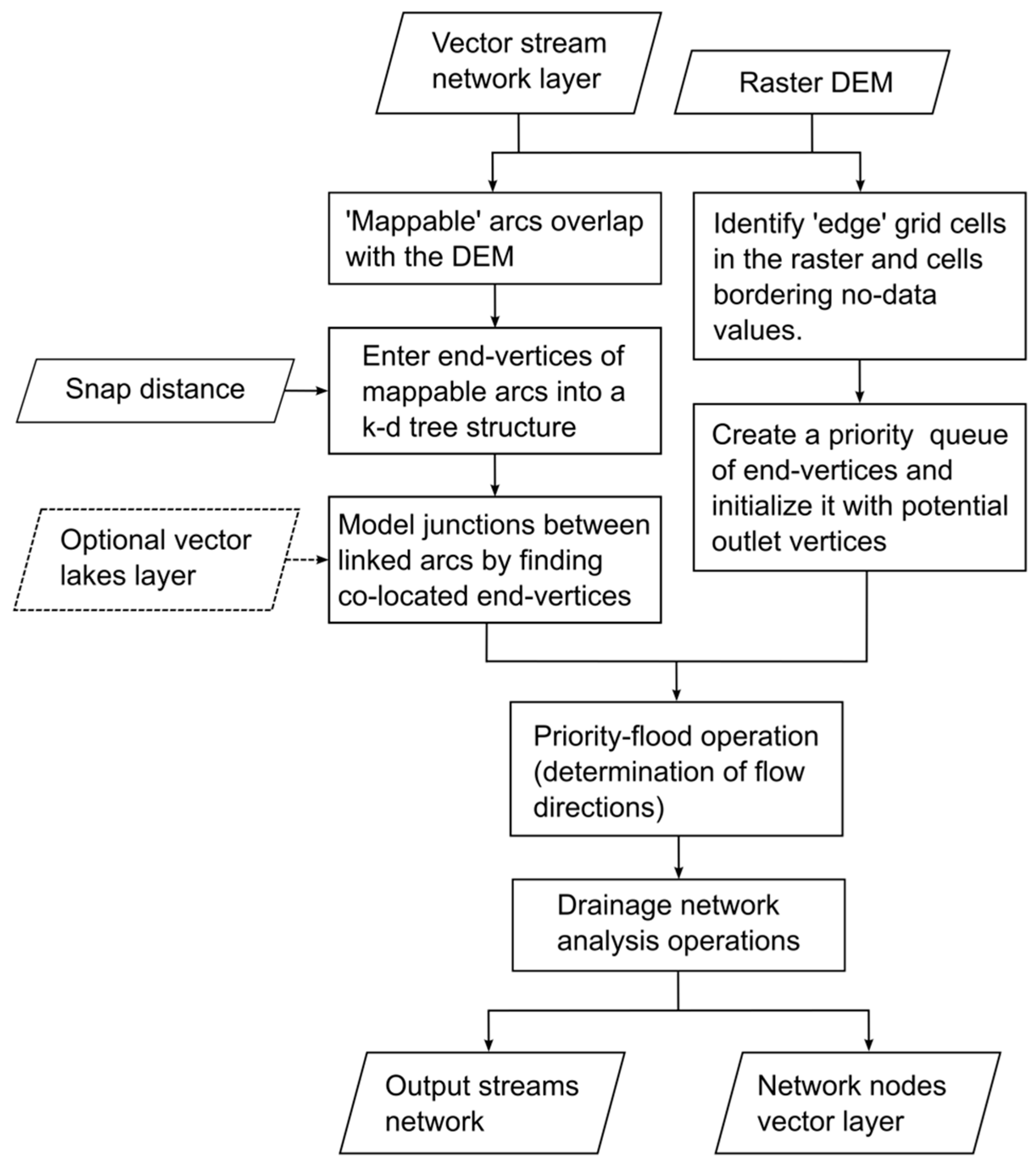
2.2. Determining Flow Directions

This study presents a novel algorithm for drainage network analysis that overcomes the aforementioned topological errors. The new algorithm has been implemented as a plugin tool within the open-source GIS Whitebox Geospatial Analysis Tool [41]. Programed in Java and distributed under an open-source license, the source code of the ‘Vector Stream Network Analysis’ tool can be accessed from the code repository on the Whitebox GAT home page (https://jblindsay.github.io/ghrg/Whitebox/index.html). Figure 1 describes the algorithm of the plugin tool. The inputs to the new algorithm include:
  • A vector stream network, in the Shapefile file format [42],
  • A raster DEM,
  • The snap-distance used to identify nearby but non-overlapping end-vertices, and
  • An optional vector file that contains lake polygons.
The DEM input is not used to extract a raster stream network or for modeling in-stream flow directions in the same way as rastaer-based drainage network analysis algorithms. Instead, the DEM is used to identify the outlets nodes in the vector data and for assigning elevations to end-vertices, which are then used during the priority-flood operation. The priority-flood operation establishes the upstream-downstream flow directions among arcs in the vector river network based on end-vertex elevations and the topological connectivity among arcs that were formed by junctions.
The algorithm begins by identifying edge grid cells in the input DEM. These include cells with no-data (null) valued neighbors and those along the edges of the raster. All of the edge cells are flagged in a temporary raster and initialized at the start of the procedure. These data serve as an input to the procedure for finding outlet nodes in the stream network. Arcs in the input stream vector are then read into memory and their lengths are stored in an array of arc objects. The arc object data structure is used to store property information for individual arcs, such as length and the various stream ordering indices. If any of the vertices in an arc overlap with valid (i.e., not no-data) data within the input DEM, the arc is processed further. Arcs that do not overlap with DEM data are not processed and they will not be included in the output streams vector file. If any of the vertices of an arc either overlap with an edge cell, or cross into an area of no-data from an area of valid data, the end-vertex of the arc that is either beyond the edge or corresponding to the lower elevation value (determined from the underlying DEM) is considered to be a potential outlet node. This does imply that care is needed in selecting the spatial extent of the DEM that is used for this analysis. If the DEM extends well beyond the vector stream network, clipping might be required; similarly, if the DEM does not overlap with significant portions of the stream vector, portions of the networks will be excluded. Outlet nodes are placed into a priority queue, with priority set by elevation. A priority queue is a data structure that is used to retrieve data in a particular order based on an index of priority. Data can be pushed into the queue in an arbitrary order and retrieved and removed (i.e., popped) in the order of their priority values. Notice that not all end-vertices that are located along the edge necessarily are actual outlets. If the river vectors extend beyond the DEM, some of the identified potential outlet nodes will belong to upstream links. The verification of an end-vertex as an outlet occurs during the priority-flood operation.
Once the potential outlets have been identified, a list of junctions is created to find arcs that are linked by co-located end-vertex coordinates. This is accomplished by placing the coordinates of each arc’s end-vertices into a k-d tree, a data structure that allows for efficient nearest-neighbor analysis. A range-search operation is performed while using the k-d tree at the coordinates of each end-vertex to identify groups of co-located vertices, with a range distance set by the snap-distance input parameter. If the range-search operation does not identify any co-located end-vertices at the location of a test point, the location is either a channel head, an outlet, or the downstream point of a stream that does not flow to the edge of the DEM. These disconnected streams are problematic for the algorithm, because their outlets cannot be readily distinguished. Disconnected streams are marked and they are included in the output streams layer.
In some cases, disconnected streams in vector hydrography data are the result of lakes. It is common practice to replace lakes (and wider rivers) in vector hydrography data with their center-line representation. Disconnected streams frequently occur where this process is incomplete and the inlets and outlets to lake features are disjoint. While it is desirable to replace lakes with centerlines for many stream network operations, the algorithm does allow for users to input an optional lakes layer. If an end-vertex is not co-located with any other vertices in the stream network, a second range operation is performed, while using a k-d tree that is populated with all lake polygon vertices, to determine whether the stream vertex is a lake inlet/outlet point. Therefore, lakes can be treated like typical confluence junctions, such that the inlets/outlets to a lake can be linked through the lake junction.
The priority-flood operation is one of the main computational tasks of the algorithm and it is the step in which flow directions (i.e., the upstream-downstream connections between links) are established. The priority-flood operation has previously been used with raster DEM data and it has not been applied to vector data in the past. It has primarily been used in algorithms for removing topographic depressions in DEMs that are applied in hydrological applications [37,38,43]. The name of the priority-flood operation comes from its reliance on a priority queue to maintain a dynamic set of features as they are encountered by the front of an artificial flood-wave associated with rising water levels. The method effectively simulates the flooding of a terrain by rising waters from an imaginary sea in the areas that extend beyond a DEM. A priority-flood operation allows for an efficient means of visiting each grid cell in a DEM in the order that they would be inundated by the inward progressing flood wave of the rising waters. In our case, instead of establishing the flood order of grid cells in a DEM, we use the same priority-flood approach to determine the flood order of end-vertices in the vector stream network. In the traditional priority-flood method, newly flooded grid cells are identified as the neighbors of previously inundated cells. By comparison, our method identifies newly flooded end-vertices through their connection with previously inundated end-vertices connected either by sharing an arc (i.e., the opposing end-vertex of an arc) or through the co-located positioning of a junction.
The priority queue that was used in the vector drainage network analysis tool is initialized with potential outlet end-vertices during the earlier step. The end-vertex within the queue with the lowest elevation (established from the underlying DEM) is then popped from the queue and all connected and previously undiscovered end-vertices are pushed into the priority queue. End-vertices are effectively flooded at the point where they are popped from the queue, at which point undiscovered end-vertices that are directly connected to the popped vertex are pushed into the queue. When a vertex is added to the queue, its associated arc object is flagged as having been discovered. As the artificial flood wave increasingly inundates headward portions of the stream network, the discovering arc is recorded as the downstream arc of newly discovered features, which establishes a flow direction for each arc in the network. This operation of popping end-vertices, identifying and adding to the queue newly discovered neighboring end-vertices, and updating the downstream flow direction information, iterates until each end-vertex has been visited, which will occur once the queue is empty. A unique outlet identifier value is assigned to each outlet vertex (i.e., one that has no established downstream connection) that is popped from the queue. As upstream connections are determined, this unique outlet identifier is propagated to connected arcs in the network, along with information regarding the distance to the outlet (relying on the arc length information) and the number of downstream links. Diffluences are identified during processing as junctions that are discovered by multiple downstream arcs possessing the same outlet value. The identification of diffluences and the ability for arc objects to store multiple downstream links in their defined flow direction are key to the representation of flow through braided sections of rivers.
Notice that the priority-flood operation approach can determine appropriate topology in the case of conjoined channel heads from adjacent catchments, which can confound some tree traversal methods. The priority-flood method can also establish flow directions without assuming consistent upstream-to-downstream (or vice versa) digitizing order among the stream arcs. The use of a k-d tree to identify junctions in the vector streams data handles topological errors that result from misaligned end-vertices. Also note that the priority-flood operation ascends each directed acyclic graph, from their outlet nodes towards the headwater links, simultaneously, rather than traversing individual graphs one at a time.

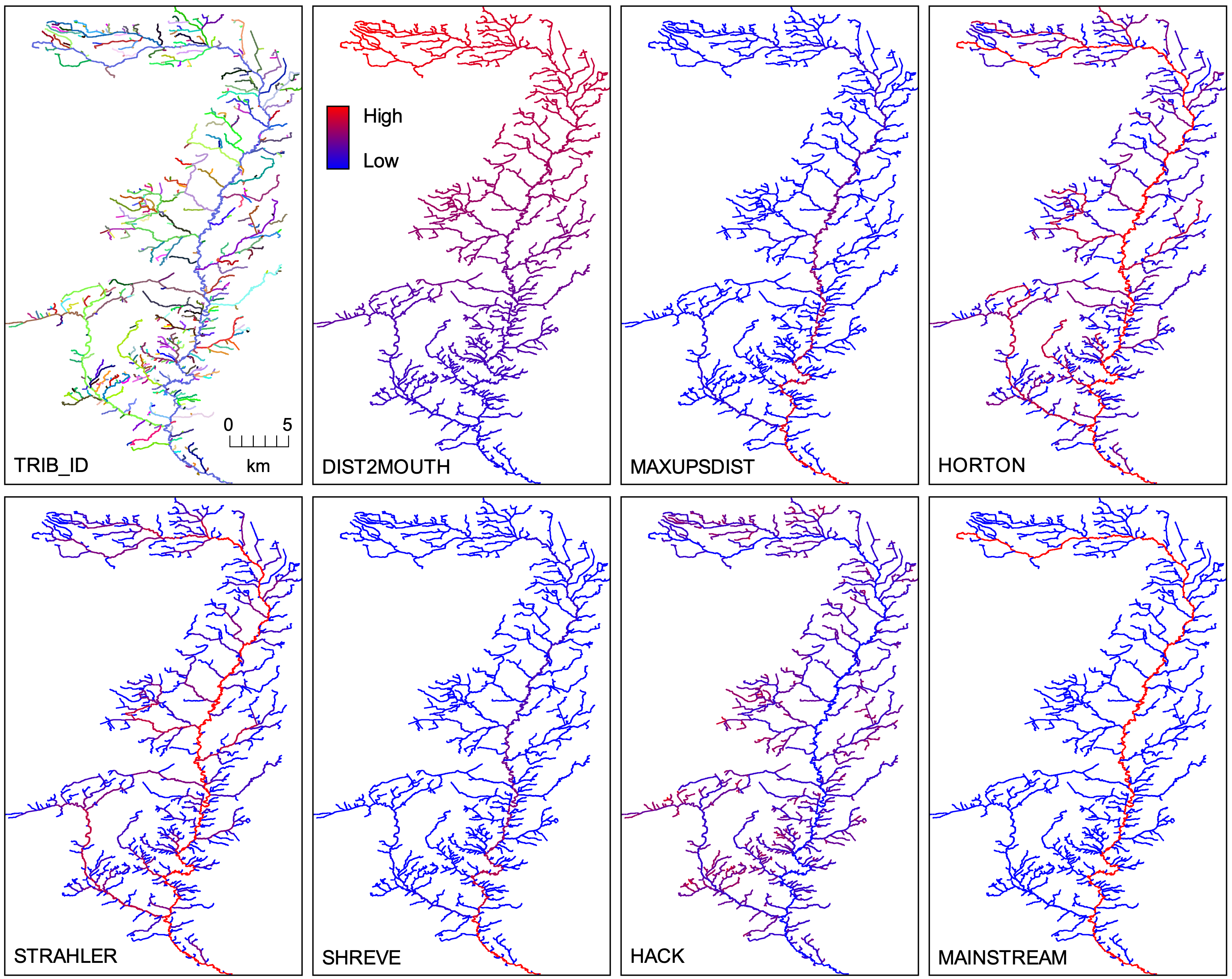
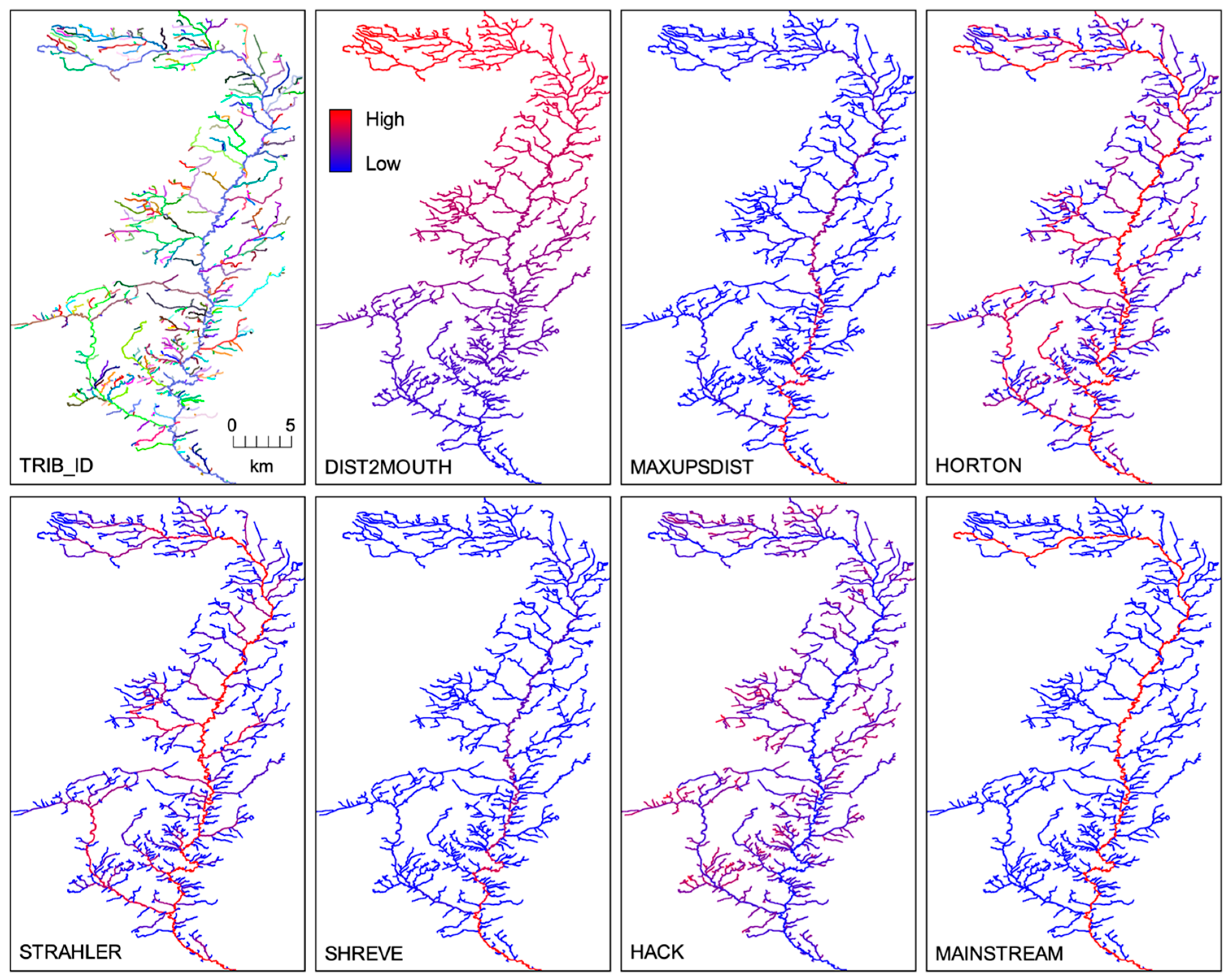
2.3. Network Analysis Indices
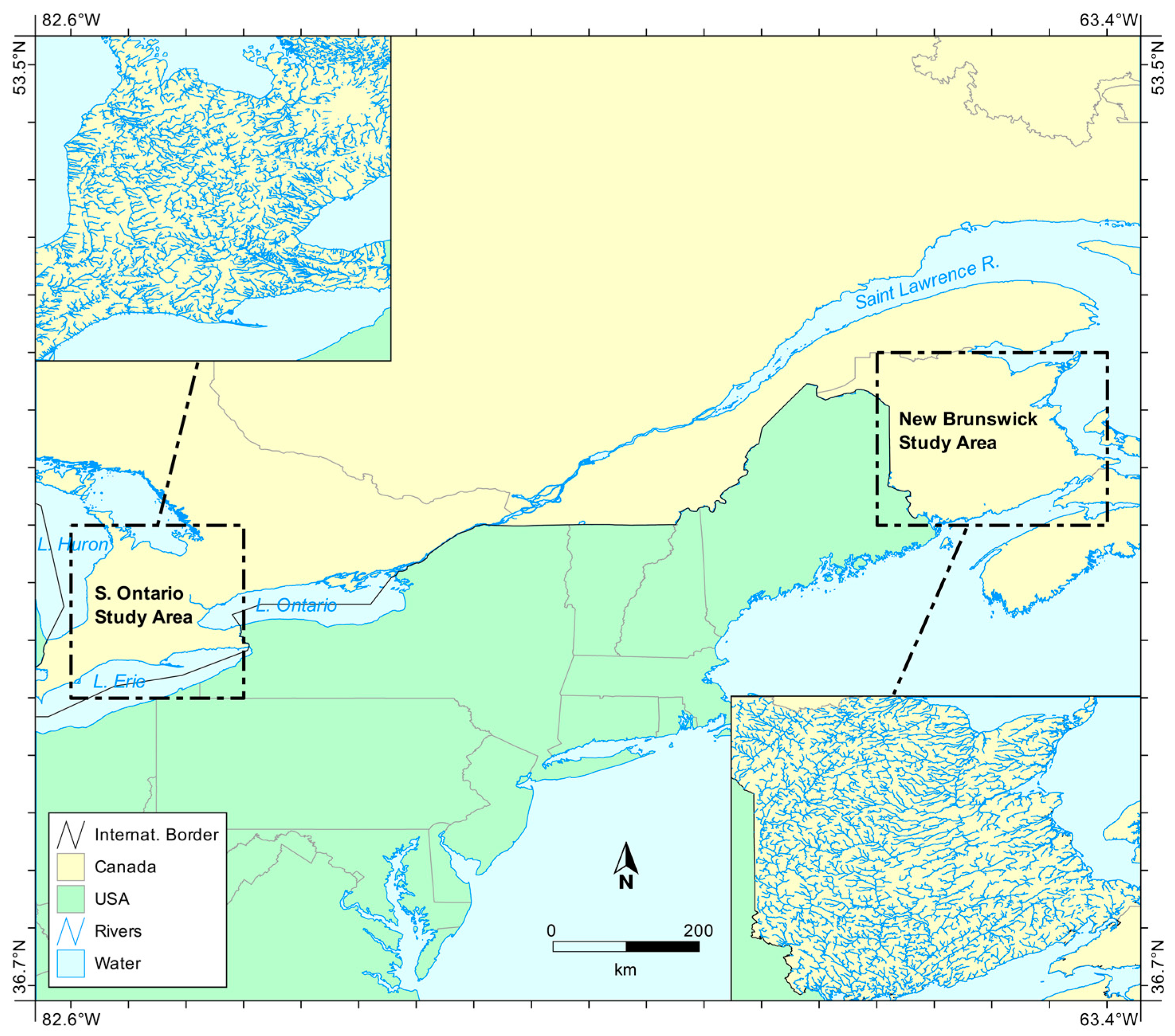
Table 1 is a listing of the network indices that the drainage network analysis tool assigns to each arc in the output stream layer. Three of the indices, OUTLET, DIST2MOUTH, and DS_NODES, are calculated during the priority-flood operation. Most of the remaining stream link indices that are described in Table 1 are calculated during a subsequent traversal from each channel head progressing downstream towards the basin outlet. This downstream progressing traversal of the stream graph works by populating an array with the number of inflowing arcs (NIA) to each arc, which is determined while using the flow direction data. Arcs for which NIA = 0 are headwater links, the identifiers of which are entered into a stack (i.e., a last-in/first-out data structure) and their index values are initialized (TUCL = link length; MAXUPSDIST = link length; STRAHLER = 1; SHREVE = 1). Each entry in the stack is then popped and their downstream arcs are identified and the values of their indices are then calculated. The NIA of downstream arcs are then decremented. When the decremented NIA value of an arc reaches zero (i.e., all upstream arcs have been popped from the stack), it is pushed onto the stack. Notice that this headwater-to-outlet traversal is non-recursive, unlike many of the tree-graph traversal algorithms that are used in many other vector drainage network analysis tools.
Calculation of TUCL is a simple accumulation operation from upstream to downstream arcs in the network. Computing MAXUPSDIST requires propagating the maximum value of each of the inflowing arcs downstream. Each headwater arc (i.e., arc with a channel head) is assigned a unique TRIB_ID during initialization and downstream arcs are assigned the TRIB_ID of the inflowing arc with the largest TUCL value. Like TUCL, SHREVE is calculated as an accumulation operation during the traversal, where the downstream arcs are assigned the sum of the SHREVE value of all inflowing arcs. Calculating STRAHLER requires the usual rules by which the value assigned to an arc is the maximum order of the inflowing arcs, and where two inflowing arcs share that value, the downstream STRAHLER order is incremented by one. Care is needed in the handling of braided river sections. Where a diffluence is encountered during the downstream traversal of the network, the upstream TUCL and SHREVE values are equally divided among all downstream arcs. This mimics the way that water flowing through the bifurcating channel is divided among the braided channels. The TRIB_ID value and STRAHLER order of the upstream arc are propagating unaltered to each downstream arc at a diffluence. Thus, an additional rule is added to the calculation of Strahler stream order, such that if two inflowing arcs share the same STRAHLER order, the downstream arc is only incremented if the TRIB_ID values of the two inflowing arcs are different. In this way, the STRAHLER order does not increase at the confluence downstream of a braided section.
Because the Horton and Hack stream ordering systems both require downstream information to be propagated upstream along tributaries (i.e., the values remains constant from a tributary’s downstream-most nodes up to its initiating channel heads), these indices must be calculated while using an outlet-to-headwaters directed traversal of the stream network after determining the TRIB_ID values. This process follows a similar method to that of the downstream-directed traversal, except that the stack is initialized with all outlet arcs and the inflowing arcs of the popped entries are pushed onto the stack.

3. Case Studies

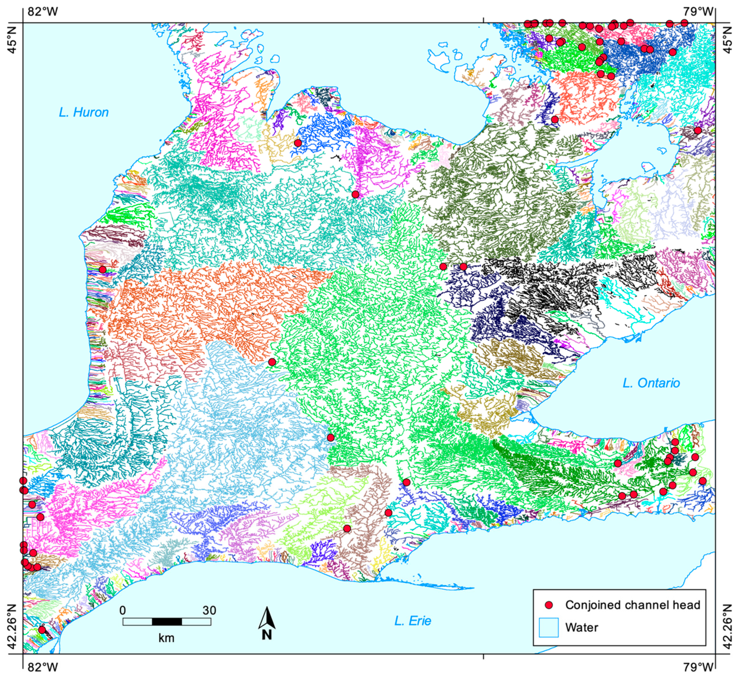
3.1. Test Sites and Data
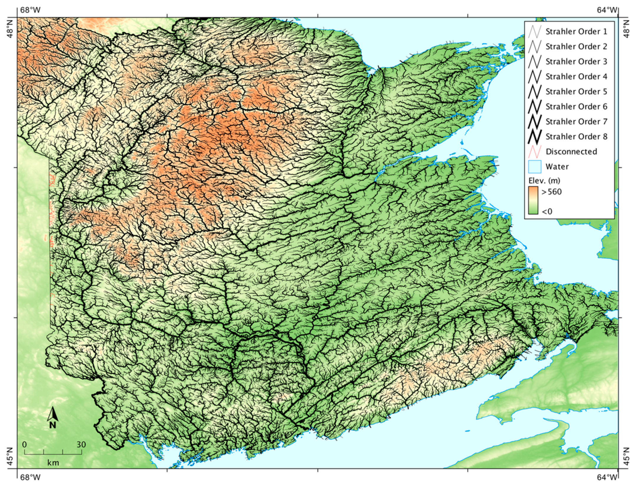
The algorithm was tested on the vector stream data of two study areas in Canada (Figure 2). The first test area was a large region (42° N to 45° N; 79° W to 82° W) within Southern Ontario, Canada, of approximately 48,000 km2. Lake Ontario and Lake Erie bound the site in the south and Lake Huron and Georgian Bay in the west and north. The major watersheds of the study area include the Grand, Thames, Saugeen, Maitland, Credit, and Humber rivers and the entire study area is part of the larger Great Lakes-Saint Lawrence system. With the exception of the deranged drainage patterns (i.e., lacking a coherent pattern) of the northeast corner of the study area (i.e., the Muskoka/Georgian Bay area situated on the Canadian Shield), rivers within Southern Ontario are generally well developed and exhibit organized drainage systems. However, the region’s watercourses do exhibit significant anthropogenic alterations, including extensive canal systems and drainage ditches.
Vector hydrographic data for the Southern Ontario study site were obtained from the 2011 Ontario Hydro Network (OHN) watercourse dataset, including detailed data layers of river systems (natural and constructed) and lakes, both of which were used in this study. The source data of the OHN was largely derived by digitizing 1:10,000 scale photogrammetrically mapped Ontario Base Maps (OBM). Attempts were made to ensure a consistent upstream-to-downstream flow direction for digitized stream links and also to replace lakes and wider rivers with their centerline representations. Initial examination of the dataset revealed that this quality assurance process was incomplete and some topological errors existed within the dataset. The streams vector contained 245,223 features within the study area and the clipped data file was 140 MB. Its size, complexity, and known topological errors made the OHN dataset a good candidate for testing the new vector drainage network analysis algorithm.
The second study area included a 72,600 km2 area (45° N to 48° N; 64° W to 68° W) within the Canadian Province of New Brunswick (Figure 2). Northerly draining rivers in the site flow into the Gulf of Saint Lawrence (including Chaleur Bay and the Northumberland Strait), while south-draining rivers flow into the Bay of Fundy on the North American Atlantic coast. The largest rivers in the study area include the Saint John River, which extends beyond New Brunswick into Maine (USA) to the west, and the Miramichi River. The St. Croix River forms the border between New Brunswick and Maine in the southwest of the study area. The 2014 New Brunswick Hydrographic Network (NBHN) watercourse data were used in this study. While the scale of the source data is not provided in the metadata, the level of detail in the streams data indicate that it was approximately 1:10,000. All the waterbodies and wider rivers were represented by their centerlines in the watercourse dataset and therefore a lakes polygon layer was not required. The original New Brunswick Stereographic (NAD83) projection of the streams data were re-projected to the common geographic coordinate system (WGS84), used for each of the data layers in this study. The vector contained 145,542 features within the study area and the clipped data file was approximately 120 MB. The western boundary of the study area intersects many of the major river systems in the site, which creates the potential for edge effects.
The input DEMs were derived from the AW3D30 global elevation data set [44], an approximately 30 m (1 arcsec) resolution elevation product created by the Japan Aerospace Exploration Agency (JAXA) using imagery from the ALOS satellite. Resampling an unreleased 5 m intermediate product created the AW3D30 DEM data. The height accuracy is estimated to be 5 m (1 sigma) and a study [45] showed that the AW3D30 product is more accurate than the comparable resolution Shuttle Radar Topography Mission (SRTM), InSAR DEMs (SRTM-1), and the ASTER Global DEM (GDEM2) 1 arcsec product. The raw data for the two study areas contained some small void areas, which were filled with the SRTM-1 data [46]. The AW3D30 data were originally acquired as individual 1° × 1° tiles, which were later mosaicked. All large waterbodies (i.e., oceans and the Great Lakes) in both of the test DEMs were replaced with no-data values. This is an important step that is needed for outlet detection in the vector drainage network analysis algorithm, as it defines the edge to which river systems drain. The input DEM for the Southern Ontario study area was a 10,800 × 10,800 raster with a 445.0 MB file size. The New Brunswick DEM was larger at 10,800 × 14,400 (rows by columns) and it was contained within a 593.3 MB data file.

3.2. Results

The tool was applied to the two input datasets using a computer system with a 2.8-GHz Intel processor with 16 GB of 1600-MHz DDR3 memory. Each of the two test datasets were processed ten times and the median computational run times were recorded. The Southern Ontario study area dataset was processed in 25.3 s, while the New Brunswick dataset required 32.0 s to process. Therefore, the Southern Ontario test data required less time to process despite its greater topological complexity, approximately 100,000 more stream features, and the additional lakes polygon layer. The longer processing time of the New Brunswick data was due to the larger raster size of its input DEM. Processing time was found to be highly dependent on DEM size, largely owing to the additional computation that is required to flag edge cells used in outlet identification with larger the DEM raster sizes (Figure 1). The DEM edge cell finding method is a basic raster scan and opportunities for parallelizing this step will be explored in a future version of the tool.
Figure 3 and Figure 4 show the results of applying the new drainage network analysis algorithm to the Southern Ontario and New Brunswick test datasets, respectively. The resulting vector drainage networks have been rendered with line thicknesses proportional to Strahler stream order. Both of the tests used a 10 m snap distance, although no mis-aligned junctions were found in either test dataset. Figure 5 provides an example of eight of the 12 drainage network indices output by the new algorithm (Table 1), applied to the vector stream data for Big Creek, a watershed draining to Lake Erie near Port Rowan, Ontario. The Southern Ontario study area contained 1524 individual basins (Figure 6), however most of these were small catchments directly draining into the Great Lakes (e.g., Figure 5). There were 49 larger basins in the site with a Horton-Strahler order of 5 or higher. The New Brunswick study area was found to contain a similar number of basins (1532), 34 of which were of order 5 or higher.
The test data for the Southern Ontario site contained 162 conjoined channel heads connecting adjacent drainage basins, including approximately ten occurrences along major regional drainage divides (Figure 6). In many instances, conjoined heads were associated with watercourses in highly modified agricultural or suburban areas. Although the number of these joins is relatively small, locating them, for manual correction, in such a large data layer would be a difficult task. By comparison, the priority-flood method locates the appropriate drainage divide between conjoined basins automatically and then saves these sites in the output nodes layer. The New Brunswick dataset did not contain any occurrences of conjoined channel heads.
The processed Southern Ontario drainage network contained 6561 disconnected stream features (0.03% of total) and the New Brunswick test resulted in 183 disconnected streams (0.001% of total). The vast majority of the disconnected streams in the Southern Ontario study area were within the area north of Toronto, along the Oak Ridges moraine (Figure 3). The hydrology along the moraine and within the heavily urbanized Greater Toronto Area is highly complex and the digitized OHN watercourse data in this region contains numerous discontinuities. Some of the disconnected streams in the OHN data resulted from missing centerlines for smaller lakes. The number of disconnected stream features in the output drainage network would have increased to 7293 without the inclusion of the optional lakes polygon layer. All of the disconnected streams in the New Brunswick dataset were situated along the western border of the study area (Figure 4). These streams belonged to smaller headwater catchments that drained to the western border of New Brunswick. The algorithm did not identify the outlets of these small drainage systems because the input DEM included the area beyond this border, i.e., none of the downstream-most links within these systems were located along the edge of the DEM data. While it would have been possible to clip the extent of the input DEM to match that of the study area, this was not performed because of the need to extend the DEM data beyond the three rivers in the area that serve as jurisdiction borders. This situation illustrates an edge effect that potentially impacts the results of the new algorithm where larger regional river systems are truncated at an unnatural boundary (i.e., not a drainage divide).
While neither of the study sites contained rivers with complex braided section, the Southern Ontario streams did contain some simple braided section. Figure 7 provides an illustration of how the algorithm assigned the same tributary identifier values to each branching reach of braided channels by recognizing stream bifurcation.
The algorithm’s method for identifying potential outlets for stream links that intersect with the DEM edge presents challenges where rivers serve as borders. This was the case for the New Brunswick study area, where three major rivers serve as the border between New Brunswick and neighboring jurisdictions. Where this occurs, it is essential that the input DEM data extends beyond the bordering river; otherwise, the algorithm will identify numerous artifact outlets along the river.
Both of the test vector stream layers contained artifact streams that connected streams beyond their natural mouths, presumably to aggregate coastal watersheds of adjacent rivers draining nearby lengths of coastline. In these coastal areas, streams were extended past their outlets some distance into the waterbodies and then joined with connecting lines parallel to the shoreline. These conjoining stream lines would make identifying outlet nodes difficult while using traditional vector drainage analysis techniques. However, because these artifacts occur beyond the edges of the DEMs (i.e., within the void areas of waterbodies), the new algorithm removes these features during the analysis. Importantly, in so doing, these coastal watersheds are individually treated rather than in aggregate.

4. Discussion

DEM-based approaches are currently widely used in applications of drainage network analysis, partly owing to the long history of development of fully automated surface flow routing methods that are based on DEMs and the ubiquitous implementation of these methods in GIS software. By comparison, vector-based drainage network analysis tools are less commonly implemented in desktop GIS (often requiring dedicated software or plugins) and frequently make restrictions on the topological properties of the input data that implies the need for some manual data preparation. The extraction of accurate river networks from DEMs remains the greatest challenge to DEM-based methods [47]. When a DEM cannot be used to extract a quality river network, often due to inadequate spatial resolution or substantial elevation error, it is a common practice to burn vector stream data into the DEM [27,48], which forces the modeled flow paths to match that of presumed higher-accuracy mapped vector hydrographic data. Stream burning can result in topological errors due to the mismatch in spatial scales between the DEM and hydrographic datasets [48]. Stream burning is essentially a technique for enhancing the representation of rivers in a DEM by combining the terrain model with mapped vector data. In many such cases where stream burning is applied, and where the aim of the application is to perform common drainage network analysis tasks (e.g., stream ordering), a better approach would be to directly analyze the vector river network.
The new vector drainage network analysis algorithm that is presented in this study uses DEM data to enhance the topological representation of flow through the vector river network and reduce the need for manual editing. Thus, rather than degrading the accuracy of the vector river network through rasterization (a necessary step during stream burning), this new technique uses the DEM to aid with the determination of flow directions within the vector stream network. In so doing, the method simplifies the topological requirements of the vector-based approach, allowing for the processing of large topologically noisy vector streams data, such as the Southern Ontario test dataset. There are many hydro-geomorphic applications of stream-burned DEMs that do not involve drainage network analysis, in which case DEM-based methods are well justified. However, this study has demonstrated the potential for using methods that combine vector streams data and DEMs, based on a vectorized version of the efficient priority-flood operation, to perform fully automated drainage network analysis.
Practitioners should consider the quality of the stream representation in all available data sets in deciding whether to adopt a DEM-based or vector-based approach to drainage network analysis. Under some conditions, stream representation is superior in available DEMs, e.g., where fine-resolution LiDAR data exist and where the available aerial photography for the area is either at a coarser resolution or heavily obscured by forest cover. In these conditions, DEM-based network analysis might be the better option for practitioners. However, in applications where available vector hydrography data are superior to the available DEM data, and where drainage network analysis (e.g., stream ordering) is the primary goal of the application, we would argue that vector-based network analysis of the type demonstrated in this study may be a better alternative to commonly used stream-burning and DEM-based approaches.

5. Conclusions

The vector drainage network analysis algorithm that is presented in this study was able to efficiently process two large stream layers of extensive geographical regions without any manual editing or data manipulation. This algorithm uses a new approach for processing vector hydrography data that is based on the priority-flood operation, commonly applied to raster DEMs. While the tool does require the input of a DEM, these data are used solely for the purposes of identifying outlets in the vector streams layer and for resolving the flood order of stream links. The new method is capable of handling topologically noisy vector hydrography data, including conditions where:
  • Stream nodes are disjoint (i.e., stream arcs are not connected end-to-end),
  • Channel heads from adjacent basins are joined,
  • Lakes have not been replaced with their centerline representation, and
  • Individual arcs in the streams layer have been digitized heterogeneously in both upstream-downstream and downstream-upstream within the same dataset.
The method was shown to be somewhat sensitive to edge effects that are related to the overlapping extent of the input vector hydrography data and the raster DEM and could not identify disconnected streams where the outlet was not located along the boundary of the DEM data. Both of these issues were related to the method by which the stream outlet nodes were located. Future work will explore possible alternative outlet identification techniques.

Author Contributions

Conceptualization, J.B.L., W.Y. and D.D.H.; Methodology, J.B.L.; Software, J.B.L. and D.D.H.; Validation, J.B.L.; Formal Analysis, J.B.L.; Investigation, J.B.L.; Resources, J.B.L.; Data Curation, J.B.L.; Writing-Original Draft Preparation, J.B.L.; Writing-Review & Editing, W.Y. and D.D.H.; Visualization, J.B.L.; Project Administration, J.B.L.; Funding Acquisition, J.B.L.

Funding

This research was funded by a grant provided by the Natural Sciences and Engineering Research Council of Canada (NSERC; grant number 400317).

Acknowledgments

The authors would like to thank the four anonymous reviewers. Their insightful comments and suggestions contributed significantly to the final form of this manuscript.

Conflicts of Interest

The authors declare no conflict of interest. The funders had no role in the design of the study; in the collection, analyses, or interpretation of data; in the writing of the manuscript, or in the decision to publish the results.

References

  1. Smart, J.S. The analysis of drainage network composition. Earth Surf. Process. 1978, 3, 129–170. [Google Scholar] [CrossRef]
  2. Horton, R.E. Erosional development of streams and their drainage basins; hydrophysical approach to quantitative morphology. GSA Bull. 1945, 56, 275–370. [Google Scholar] [CrossRef]
  3. Kirkby, M.J. Tests of the random network model, and its application to basin hydrology. Earth Surf. Process. 1976, 1, 197–212. [Google Scholar] [CrossRef]
  4. Naden, P.S. Spatial variability in flood estimation for large catchments: The exploitation of channel network structure. Hydrol. Sci. J. 1992, 37, 53–71. [Google Scholar] [CrossRef]
  5. Rice, J.S.; Emanuel, R.E.; Vose, J.M. The influence of watershed characteristics on spatial patterns of trends in annual scale streamflow variability in the continental U.S. J. Hydrol. 2016, 540, 850–860. [Google Scholar] [CrossRef]
  6. Rodriguez-Iturbe, I.; Valdés, J.B.; Rodríguez-Iturbe, I. The geomorphologic structure of hydrologic response. Water Resour. Res. 1979, 15, 1409–1420. [Google Scholar] [CrossRef] [Green Version]
  7. Stenger-Kovács, C.; Tóth, L.; Tóth, F.; Hajnal, E.; Padisák, J. Stream order-dependent diversity metrics of epilithic diatom assemblages. Hydrobiologia 2014, 721, 67–75. [Google Scholar] [CrossRef]
  8. Vannote, R.L.; Minshall, G.W.; Cummins, K.W.; Sedell, J.R.; Cushing, C.E. The river continuum concept. Can. J. Fish. Aquat. Sci. 1980, 37, 130–137. [Google Scholar] [CrossRef]
  9. Strahler, A.N. Quantitative analysis of watershed geomorphology. Trans. Am. Geophys. Union 1957, 38, 913–920. [Google Scholar] [CrossRef]
  10. Shreve, R.L. Statistical law of stream numbers. J. Geol. 1966, 74, 17–37. [Google Scholar] [CrossRef]
  11. Hack, J.T. Studies of Longitudinal Stream Profiles in Virginia and Maryland; US Government Printing Office: Washington, DC, USA, 1957; Volume 294.
  12. Dawson, F.; Hornby, D.; Hilton, J. A method for the automated extraction of environmental variables to help the classification of rivers in Britain. Aquat. Conserv. Mar. Freshw. Ecosyst. 2002, 12, 391–403. [Google Scholar] [CrossRef]
  13. Lanfear, K.J. A fast algorithm for automatically computing strahler stream order 1. JAWRA J. Am. Water Resour. Assoc. 1990, 26, 977–981. [Google Scholar] [CrossRef]
  14. Band, L.E. Extraction of Channel Networks and Topographic Parameters from Digital Elevation Data. In Channel Network Hydrology; Bevin, K., Kirkby, M.J., Eds.; Wiley: New York, NY, USA, 1993; pp. 13–42. [Google Scholar]
  15. O’Callaghan, J.F.; Mark, D.M. The extraction of drainage networks from digital elevation data. Comput. Vis. Graph. Image Process. 1984, 28, 323–344. [Google Scholar] [CrossRef]
  16. Seibert, J.; McGlynn, B.L. A new triangular multiple flow direction algorithm for computing upslope areas from gridded digital elevation models. Water Resour. Res. 2007, W04501. [Google Scholar] [CrossRef]
  17. Tarboton, D.G. A new method for the determination of flow directions and upslope areas in grid digital elevation models. Water Resour. Res. 1997, 33, 309–319. [Google Scholar] [CrossRef] [Green Version]
  18. Tarboton, D.; Ames, D.P. Advances in the Mapping of Flow Networks from Digital Elevation Data. In Proceedings of the World Water and Environmental Resources Congress, Orlando, FL, USA, 20–24 May 2001; pp. 1–10. [Google Scholar]
  19. Jenson, S.K.; Domingue, J.O. Extracting topographic structure from digital elevation data for geographic information system analysis. Photogramm. Eng. Remote Sens. 1988, 54, 1593–1600. [Google Scholar]
  20. Band, L.E. A terrain-based watershed information system. Hydrol. Process. 1989, 3, 151–162. [Google Scholar] [CrossRef]
  21. Lin, W.T.; Chou, W.C.; Lin, C.Y.; Huang, P.H.; Tsai, J.S. Automated suitable drainage network extraction from digital elevation models in Taiwan’s upstream watersheds. Hydrol. Process. 2006, 20, 289–306. [Google Scholar] [CrossRef]
  22. Istanbulluoglu, E.; Tarboton, D.; Pack, R.T.; Luce, C. A probabilistic approach for channel initiation. Water Resour. Res. 2002, 38, 61-1–61-14. [Google Scholar] [CrossRef]
  23. McMaster, K.J. Effects of digital elevation model resolution on derived stream network positions. Water Resour. Res. 2002, 38, 13-1–13-8. [Google Scholar] [CrossRef]
  24. Montgomery, D.R.; Foufoula-Georgiou, E.; Foufoula-Georgiou, E. Channel network source representation using digital elevation models. Water Resour. Res. 1993, 29, 3925–3934. [Google Scholar] [CrossRef]
  25. Lindsay, J.B. Sensitivity of channel mapping techniques to uncertainty in digital elevation data. Int. J. Geogr. Inf. Sci. 2006, 20, 669–692. [Google Scholar] [CrossRef]
  26. Lindsay, J.B.; Evans, M.G. The influence of elevation error on the morphometrics of channel networks extracted from DEMs and the implications for hydrological modelling. Hydrol. Process. 2008, 22, 1588–1603. [Google Scholar] [CrossRef]
  27. Saunders, W.; Maidment, D. Grid-Based Watershed and Stream Network Delineation for the San Antonio-Nueces Coastal Basin. In Proceedings of the Proceedings of Texas Water ’95: A Component Conference of the First International Conference of Water Resources Engineering, San Antonio, TX, USA, 14–18 August 1995. [Google Scholar]
  28. Garbrecht, J.; Martz, L.W. The assignment of drainage direction over flat surfaces in raster digital elevation models. J. Hydrol. 1997, 193, 204–213. [Google Scholar] [CrossRef]
  29. Nardi, F.; Grimaldi, S.; Santini, M.; Petroselli, A.; Ubertini, L. Hydrogeomorphic properties of simulated drainage patterns using digital elevation models: The flat area issue. Hydrol. Sci. J. 2008, 53, 1176–1193. [Google Scholar] [CrossRef]
  30. Grimaldi, S.; Nardi, F.; Di Benedetto, F.; Istanbulluoglu, E.; Bras, R.L. A physically-based method for removing pits in digital elevation models. Adv. Water Resour. 2007, 30, 2151–2158. [Google Scholar] [CrossRef]
  31. Kenny, F.; Matthews, B.; Todd, K. Routing overland flow through sinks and flats in interpolated raster terrain surfaces. Comput. Geosci. 2008, 34, 1417–1430. [Google Scholar] [CrossRef]
  32. Woodrow, K.; Lindsay, J.B.; Berg, A.A. Evaluating DEM conditioning techniques, elevation source data, and grid resolution for field-scale hydrological parameter extraction. J. Hydrol. 2016, 540, 1022–1029. [Google Scholar] [CrossRef]
  33. Gleyzer, A.; Denisyuk, M.; Rimmer, A.; Salingar, Y. A fast recursive gis algorithm for computing strahler stream order in braided and nonbraided networks. JAWRA J. Am. Water Resour. Assoc. 2004, 40, 937–946. [Google Scholar] [CrossRef]
  34. Hornby, D. RivEX. Available online: http://www.rivex.co.uk/ (accessed on 5 September 2019).
  35. Holloway, R. Using RivEX and National Hydro Network Data to Classify Water Quality Stations by Strahler Stream Order; Government of Newfoundland and Labrador: St. John’s, NL, Canada, 2009.
  36. Pradhan, M.P. Automatic Association of Stream Order for Vector Hydrograph using Spiral Traversal Technique. IOSR J. Comput. Eng. 2012, 1, 9–12. [Google Scholar] [CrossRef]
  37. Barnes, R.; Lehman, C.; Mulla, D. Priority-flood: An optimal depression-filling and watershed-labeling algorithm for digital elevation models. Comput. Geosci. 2014, 62, 117–127. [Google Scholar] [CrossRef] [Green Version]
  38. Soille, P.; Gratin, C. An Efficient Algorithm for Drainage Network Extraction on DEMs. J. Vis. Commun. Image Represent. 1994, 5, 181–189. [Google Scholar] [CrossRef]
  39. Heckmann, T.; Schwanghart, W.; Phillips, J.D. Graph theory—Recent developments of its application in geomorphology. Geomorphology 2015, 243, 130–146. [Google Scholar] [CrossRef]
  40. Peckham, S.D.; Gupta, V.K. A reformulation of Horton’s laws for large river networks in terms of statistical self-similarity. Water Resour. Res. 1999, 35, 2763–2777. [Google Scholar] [CrossRef]
  41. Lindsay, J. Whitebox GAT: A case study in geomorphometric analysis. Comput. Geosci. 2016, 95, 75–84. [Google Scholar] [CrossRef]
  42. ESRI Shapefile Technical Description: ESRI White Paper. Available online: https://www.esri.com/library/whitepapers/pdfs/shapefile.pdf (accessed on 17 September 2019).
  43. Lindsay, J.B. Efficient hybrid breaching-filling sink removal methods for flow path enforcement in digital elevation models. Hydrol. Process. 2016, 30, 846–857. [Google Scholar] [CrossRef]
  44. Tadono, T.; Ishida, H.; Oda, F.; Naito, S.; Minakawa, K.; Iwamoto, H. Precise Global DEM Generation by ALOS PRISM. ISPRS Ann. Photogramm. Remote Sens. Spat. Inf. Sci. 2014, 2, 71–76. [Google Scholar] [CrossRef]
  45. Santillan, J.; Makinano-Santillan, M. Vertical accuracy assessment of 30-m resolution alos, aster, and srtm global dems over northeastern mindanao, philippines. ISPRS Int. Arch. Photogramm. Remote Sens. Spat. Inf. Sci. 2016, 149–156. [Google Scholar] [CrossRef]
  46. Jarvis, A.; Reuter, H.I.; Nelson, A.; Guevara, E. Hole-filled SRTM for the globe Version 4. 2008. Available online: http://srtm. csi. cgiar. org (accessed on 17 September 2019).
  47. Lai, Z.; Li, S.; Lv, G.; Pan, Z.; Fei, G. Watershed delineation using hydrographic features and a DEM in plain river network region. Hydrol. Process. 2016, 30, 276–288. [Google Scholar] [CrossRef]
  48. Lindsay, J.B.; Lindsay, J. The practice of DEM stream burning revisited. Earth Surf. Process. 2016, 41, 658–668. [Google Scholar] [CrossRef]
Figure 1. The priority-flood based vector drainage network analysis algorithm.
Ijgi 08 00422 g001
Figure 2. The locations of two study areas (marked by thick dashed black lines) used in testing the new vector drainage network analysis algorithm. The top inset map details the major drainage features of the Southern Ontario study area and the bottom inset details the New Brunswick site.
Ijgi 08 00422 g002
Figure 3. Southern Ontario study area drainage network with line thickness proportional to Strahler stream order.
Ijgi 08 00422 g003
Figure 4. New Brunswick study area drainage network with line thickness proportional to Strahler stream order.
Ijgi 08 00422 g004
Figure 5. Indices output by the drainage network analysis algorithm for Big Creek, Ontario. Index names and interpretations are provided in Table 1. TRIB_ID uses random colors to designate tributaries; the stream trunk (MAINSTREAM) is colored red while minor tributaries are blue; each of the other indices are shaded from blue (low) to red (high) and scaled to their index value ranges.
Ijgi 08 00422 g005
Figure 6. Basins and conjoined channel heads within the Southern Ontario study area. Each unique outlet identifying value is rendered in a randomly assigned color.
Ijgi 08 00422 g006
Figure 7. Tributary identifier values (designated by random colors) assigned to a braided reach of the Saugeen River, Ontario, and some of its minor tributary streams. Notice the three small braided sections situated along the main (light blue) river.
Ijgi 08 00422 g007
Table 1. Calculated drainage network analysis outputs, including their abbreviated names as they appear in the output stream layer’s attribute table.
Index NameDescription
OUTLETUnique outlet identifying value, used as basin identifier
TRIB_IDUnique tributary identifying value
DIST2MOUTHDistance to outlet (i.e., mouth node)
DS_NODESNumber of downstream nodes
TUCLTotal upstream channel length; the channel equivalent to catchment area
MAXUPSDISTMaximum upstream distance
HORTONHorton stream order
STRAHLERStrahler stream order
SHREVEShreve stream magnitude
HACKHack main stream order
MAINSTREAMBoolean value indicating whether link is the main stream trunk of its basin
DISCONTBoolean value indicating whether link is disconnected, i.e., does not drain to the edge of the DEM and no outlet could be identified

