Abstract
Flood simulations are vital to gain insight into possible dangers and damages for effective emergency planning. With flexible and natural ways of visualizing water flow, more precise evaluation of the study area is achieved. In this study, we describe a method for flood visualization using both regular and adaptive grids for position-based fluids method to visualize the depth of water in the study area. The mapping engine utilizes adaptive cell sizes to represent the study area and utilizes Jenks natural breaks method to classify the data. Predefined single-hue and multi-hue color sets are used to generate a heat map of the study area. It is shown that the dynamic representation benefits the mapping engine through enhanced precision when the study area has non-disperse clusters. Moreover, it is shown that, through decreasing precision, and utilizing an adaptive grid approach, the simulation runs more efficiently when particle interaction is computationally expensive.
1. Introduction
Throughout history, floods have been an integral part of our lives. Floods are major disasters that have been responsible for the loss of millions of lives and the collapse of cities. For centuries, we have been trying to fight against this natural disaster by utilizing a variety of strategies. Although storm surges are responsible for most of the casualties, it is noted that prolonged periods of rainfall may cause significant damage as well. An earlier example of such a disaster is known as St. Mary Magdalene’s flood, which occurred in 1342, causing thousands of deaths. The flood caused damage or total destruction on many buildings, bridges and mills. The issue with the St. Mary Magdalene’s flood is that the dry soil, which was caused due to heat and partial drought, was unable to absorb the waters, causing a devastating soil erosion [1]. With the introduction of modern road networks, additional parameters were introduced that would reshape emergency management efforts. Recent studies show that, although flooding may not be totally prevented, proper coordination of entities in emergency management can significantly relieve the damage and issues caused by it [2]. Consequently, developing new modeling approaches and tools is vital to keep our lives intact and our cities resilient.
Fluid modeling requires a detailed representation of fluids in general. Various approaches have been proposed to increase efficiency and to reduce redundancies while attaining an accurate simulation. When visual representation is important, solvers mainly focus on solving Eulerian equations [3] or Navier-Stokes equations [4]. Several other methods including Lattice-Boltzmann methods [5] also work well for fluid simulation. Consequently, it is acceptable to consider different methods for flood simulation. Some prominent approaches in this category are SPH [6], position-based fluids (PBF) [7] and mesh-free vortex particles (vortons) [8].
Since the introduction of SPH by Gingold and Monaghan [6] and Lucy [9], it has been used in a variety of industries, including computer graphics. It is a mesh-free particle-based method based on Lagrangian formulation. As SPH is Lagrangian in nature, it is not constrained by a mesh, which is its main strength. This sets it apart from grid-based approaches, which suffer from loss of mass and inflexibility due to discretizing the study area into grids. However, neighborhood is a vital part of SPH and it is generally associated with its inefficiency for real-time simulation of large environments [10]. As the value of a variable at a particle of interest can be found by checking its neighbors, efficient algorithms of reducing neighborhood dependencies is vital. There are other approaches like position-based fluids [7] that improve some of the shortcomings of SPH. Nevertheless, SPH and its variants have been commonly used in 3D flood visualization.
Through the advancement of modern graphical processing units (GPUs) and aforementioned methods of fluid description, 2D and 3D visualization have been utilized in flood modeling and analysis. Teng et al. [11] introduce state-of-the-art empirical, hydrodynamic and simplified methods used in flood modeling and underline that hydrodynamic models utilizing 2D and 3D simulations may prove to be better in representing detailed flow dynamics. Furthermore, simplified models are best used for probabilistic flood risk assessment. Leskens et al. [12] present a system for analyzing flooding scenarios through 3D visualization. Upon representing the virtual environment, numerical methods that solve 2D hydraulic equations for water flow are used to simulate the flood. It is noted that 3D representation of the flood helps practitioners to better realize and estimate the impact of a flood. Such surveys point out the power of 2D and 3D visualization in describing flooding.
Due to this power of visualization, many works proceed with various ways, simulation methods, and dynamic parameters to display the properties, which would be difficult to see otherwise. 2D and 3D models have been used for storm surge flood routing visualization [13], risk estimation [14], flood modeling and analysis [12,15,16], rainfall forecasting [17], landslide simulation [18] and to visualize many other scenarios. Recent works show a move from static visualization to dynamic visualization [19,20,21], to provide more interactive and accessible simulation tools to incorporate virtual environments and dynamic simulation parameters.
As depth, or water level, is a significant parameter to estimate risk and damage, it is vital to be able to track the water flow while computing and visualizing water levels [22,23]. Nevertheless, 3D representation may distort or complicate human-readability of the study area and therefore, it might be significant to provide 2D representation of flooding alongside 3D information [21]. 3D simulation methods can still be utilized in 2D visualization of the environment to describe flooding [24]. Although 3D representation may carry more in terms of data and offer better compression [21], 2D representation can provide better performance [11] as less data is considered.
In our work, considering state-of-the-art approaches discussed, we utilized position-based fluids [7] for simulating flood, which consider a Lagrangian description and provide certain benefits over traditional SPH [6] methods. On top of the simulation engine, we implemented a 2D mapping engine that can keep track of the flood, while generating a heat map of the study area, to visualize water depth in 2D for ease of understanding. As the simulation takes place, our dynamic mapping engine can decide on representing the flood using a regular grid or an adaptive grid. The dynamic approach helps with accuracy on demand, while keeping the simulation efficient when the situation arises.
Our mapping engine, which has the power to decide the method of representation considering environmental parameters and computational expense, provides an efficient and optimized approach to visualize water flow for flood analysis. Furthermore, our visualization approach provides a framework for mapping the depth of any 2D or 3D Lagrangian, particle-based water flow simulation, which is important for flooding scenarios. The engine provides a flexible mapping experience by utilizing Jenks natural breaks for classification, and coloring the generated depth map with predefined single-hue and multi-hue color schemes to enhance readability of the depth map [25].
In Section 2, we briefly introduce the system design. Section 3 and Section 4 discuss the individual stages of component reader, scene creator and adaptive mapping engine. Section 5 contains results generated by the mapping engine and provides figures for comparison purposes. Lastly, we conclude with Section 6 and discuss potential future work.
2. System Design
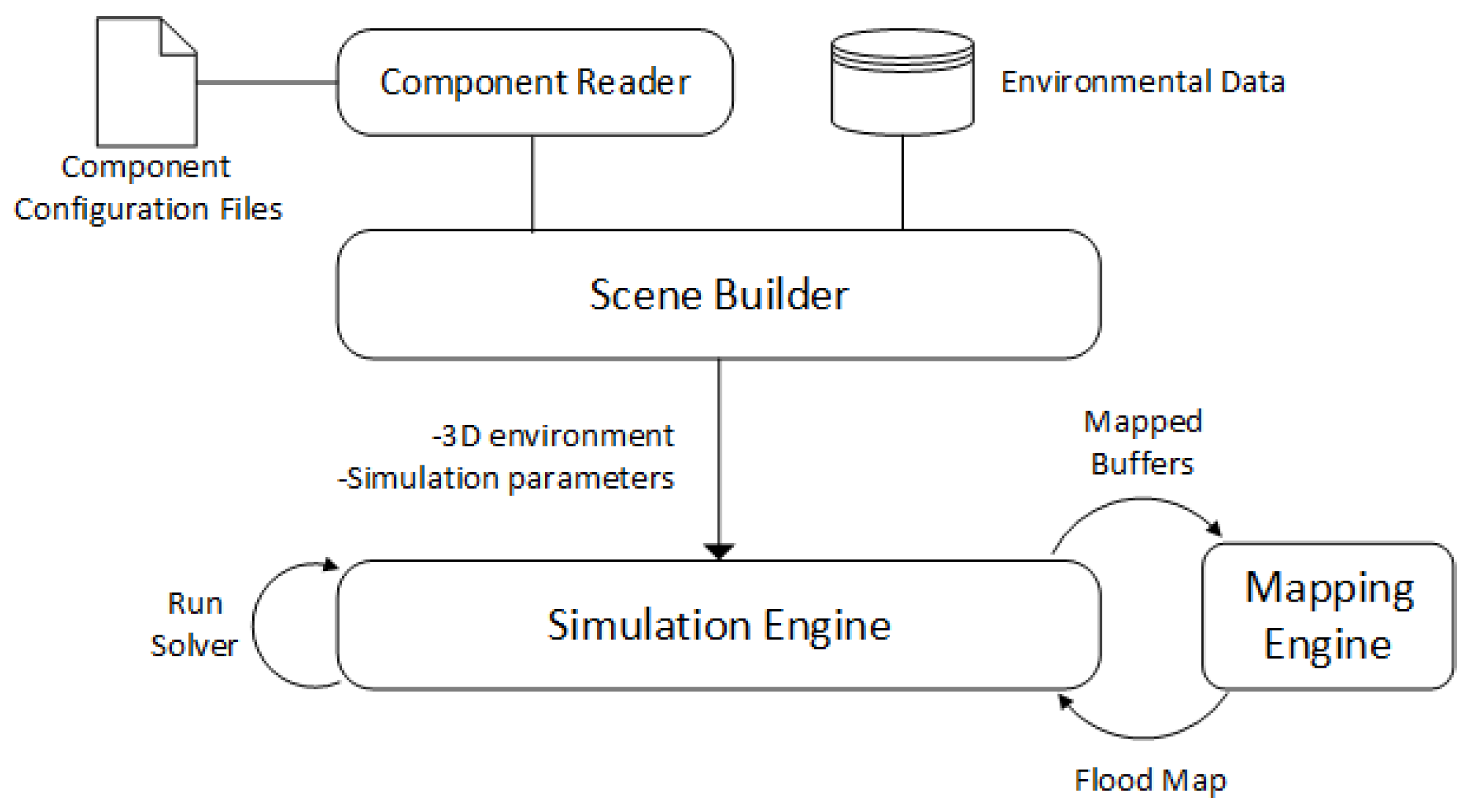
Our system consists of multiple layers for better modularity. Initially our scene descriptions are read by the scene builder, which is responsible for initializing parameters to start the simulation. After the terrain data is analyzed and a height map is produced, simulation begins. As the fluid travels on the terrain, the depth analyzer is executed every second to evaluate the particles and draw the map of the environment. Figure 1 shows an overview of the system layers.
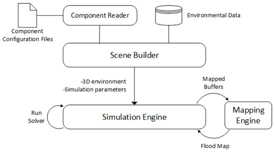
Figure 1.
Overview of the system design and data flow.
As the system focuses on optimizing performance, it executes particle mapping and depth analysis at certain intervals. The depth map of the environment can be produced using both fixed-size cells and quadtrees and therefore, depending on the problem domain, the system is able to choose an appropriate method of representation. Once the depth map is generated, the mapping engine draws a heat map using Jenks natural breaks classification method. This map can then be sent as an output for further evaluation or it can be viewed as the simulation is running for the purpose of evaluating the fluid flow.
3. Component Readers and Scene Processing
There are several components that are required for the mapping engine to properly analyze the environment. The component reader contains a set of tools to read necessary data files and place them into a container so that they can be passed to the next phase, which is the simulation itself. There are submodules that parse different types of files, such as cloud animation data, environmental configuration data, and object configuration data.
In the earliest stage, a scene description is provided to the component reader. The component reader then executes several commands step-by-step to load the data and arrange the definitions into a meaningful description. Environmental configuration data includes several parameters, such as the borders of the scene, terrain to be used in the simulation, and the rainfall speed. These parameters are then packaged into an environment structure to be passed to the simulation engine, which utilizes the position-based fluids approach to simulate water motion. Next, object configuration data is read and if needed, certain changes are done to the scene. In this phase, external entities, such as buildings, cars or trees with their simulation parameters can be imported into the scene. Upon importing these entities, the simulation terrain can be merged with these objects. If not requested, the objects stay on their own with no connection to the terrain. Lastly, cloud configuration data is read by the component reader. Cloud configuration data has information about cloud positions, rainfall intensities and their potential travel path. A dynamic description of the environment allows for more interactivity and therefore, the cloud configuration files have an animation section, in which we can place keyframes and provide translation and scale matrices to define a dynamic scene.
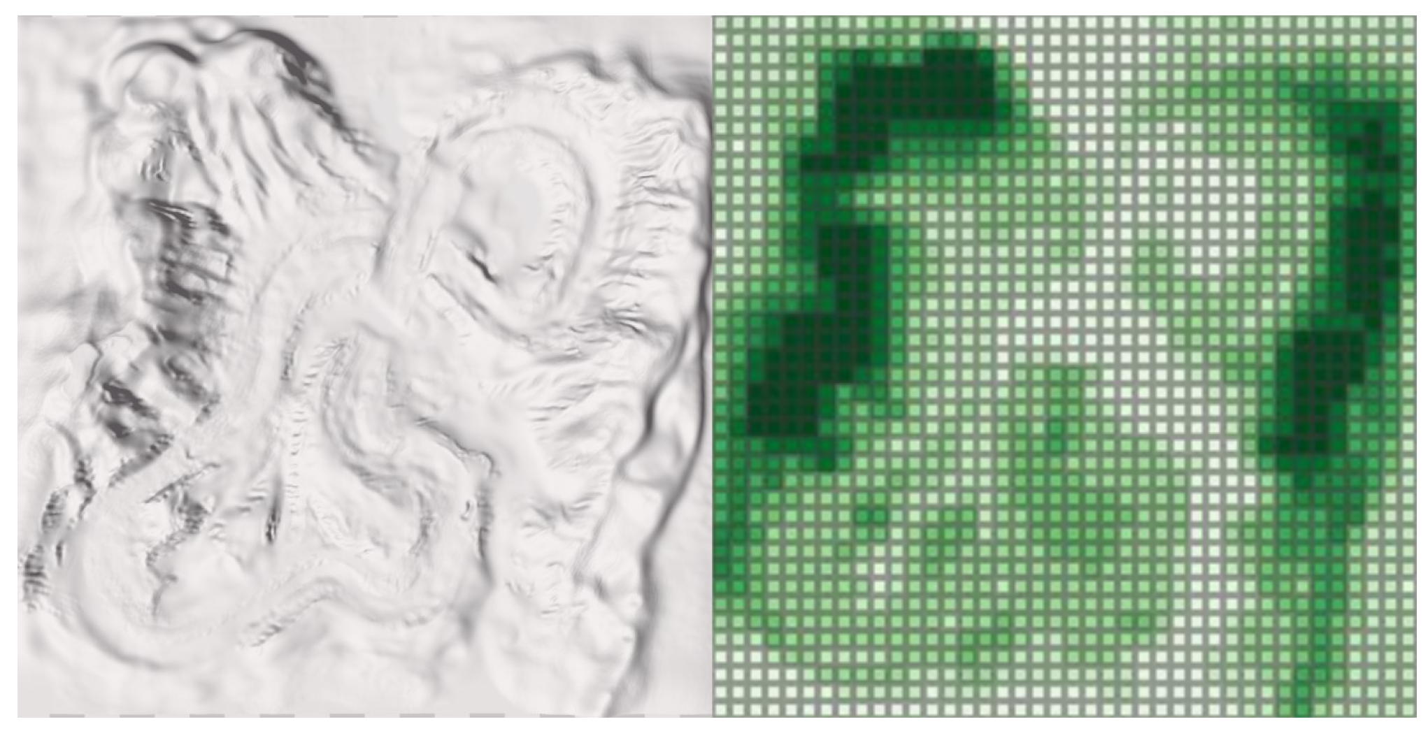
Once the component reader processes the files, these structures are then sent to the simulation engine. Before any simulation begins, a height map for the environment is generated to be used for computations at a later time. One limitation of this approach is that the terrain map is not regenerated with environmental alterations; the terrain is considered as an immovable object and thus, it is not subject to change. Naturally, this comes with an advantage of processing efficiency as the height map is generated before the simulation begins. Figure 2 shows a sample height map and the environment it was extracted from.

Figure 2.
A test environment and extracted height map on 40 × 40 regular grid.
At this point, it is worth underlining that the height map information is not yet passed to the mapping engine and therefore, it is just stored as a structure within memory. When the mapping engine requests the data, the structure is passed and utilized by the engine, whether it is for visualizing the height of the environment, as shown in Figure 2, or just to utilize the data for calculating water depth.
4. Map Generation and Visualization
The implementation of the mapping engine and algorithms utilized to generate the maps are considered with an emphasis on performance and accurate visualization. The engine is able to recognize and reason about the environment that it is mapping through analysis of several environmental parameters. Upon evaluation, an appropriate representation is selected and map information is passed back to the simulation engine for viewing purposes. Moreover, the engine is able to process and extract the map data if requested.
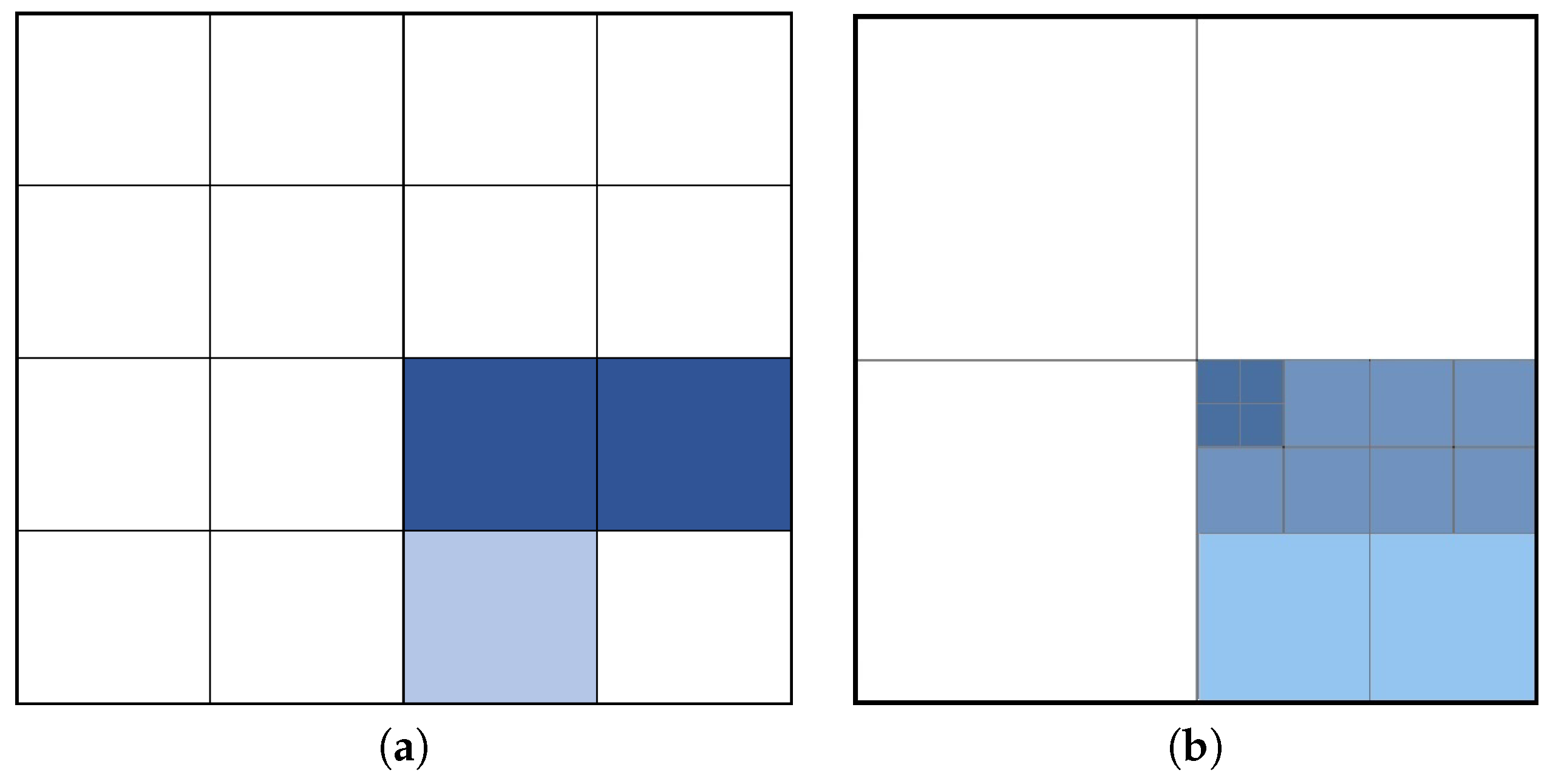
The mapping engine considers two major representations of discretization: regular and adaptive grids. Depending on the environmental parameters and the way the fluid behaves in the simulation, the engine is able to switch from one representation to the other. For performance purposes the engine is, if instructed, able to make changes to the maximum number of cells it is utilizing to make the simulation run faster. As quadtrees are used to implement the adaptive grid, the engine also tracks the number of cells and depth of each subtree. The initial parameters regarding maximum number of cells, rows, columns and maximum depth are derived from the boundaries of the study area. Depending on the size and the shape of the environment, appropriate values are determined. These two approaches are shown in Figure 3.

Figure 3.
Area representation using (a) regular grid, (b) adaptive grid.
Regular grids are commonly used where the fluid particles are stretched across the study area. These grids help the system focus on each region equally, which may visualize the bodies of water more accurately. Although it is wasteful in terms of storage and in some cases less precise as a limit is applied to the maximum number of cells, it is valuable when the study area receives fluid particles in its entirety. The engine prefers this algorithm when the study area is small; the fluid that gets distributed across the entire map, or body of water, such as a lake or an ocean, is defined as the main terrain of the scene. Once a regular grid is selected, the engine tries to minimize the number of stuck particles from being included in the computation and therefore, it removes particles located below the reference point, which is provided as an input for the simulation engine.
Adaptive grids have their own advantages in terms of representation. Firstly, their nature enables the engine to optimize storage and increase the speed of fluid visualization on demand. This approach is best utilized when there are specific regions with significant fluid interaction in the study area, while the rest remains relatively stable. When such clusters occur, the engine uses adaptive cells to describe the areas with fluid interaction similar to regular grids with little or no loss of precision in representation. Therefore, it provides better performance due to stable regions not being discretized. Moreover, as indicated earlier, the engine is able to make a transition between the two approaches and change the level of precision depending on the number of particles and simulation performance, to make the mapping process execute faster.
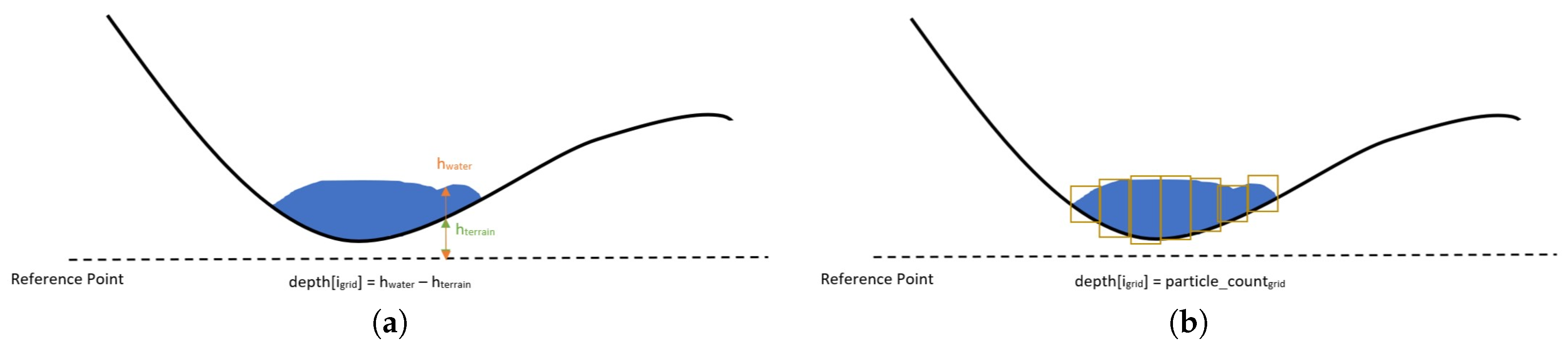
Depth values are estimated through two different approaches. A relative difference method is used on demand, to calculate the difference between the height of water and the height of the terrain submerged in water. The height values are computed considering a reference point, which is passed as a scene configuration parameter. The engine calculates a depth value for each grid cell and then passes the depth map as the input for the next stage. Furthermore, the engine can compute the depth map using number of particles as the main indicator of flooding. With this approach, the engine counts the number of particles clustered in each cell and then produces a volume-based depth value. Upon computation of the values for each grid, the depth map is passed to the next stage. As a performance optimization, the system considers all objects except fluid particles as immobile and consequently, it cannot track soil erosion or object translation from one point to another. Figure 4 shows the visualization of these different approaches.
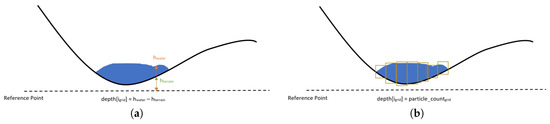
Figure 4.
Computation of depth using (a) relative height differences, (b) fluid volume through number of particles per grid.
For proper depth computation, several conditions must be kept track of. The fluid particles, as they are dynamic, update their positions, velocities, and other parameters depending on the environmental conditions. Before any attempt is made to compute depth, these parameters must be updated, or mapped so that the current values are taken into account. Therefore, with a specified interval as parameter, the particles are mapped to their current state and then the data is passed to compute depth. This process can be executed per second or several milliseconds. For performance purposes, it is best to make rare updates, but for real-time tracking this may be impossible. If the demand is to map once every few seconds, snapshots of the study area can be extracted for later use. This is useful if real-time tracking is not a concern. If tracking is required, then the system finds an optimum refresh rate to keep the simulation running smoothly.
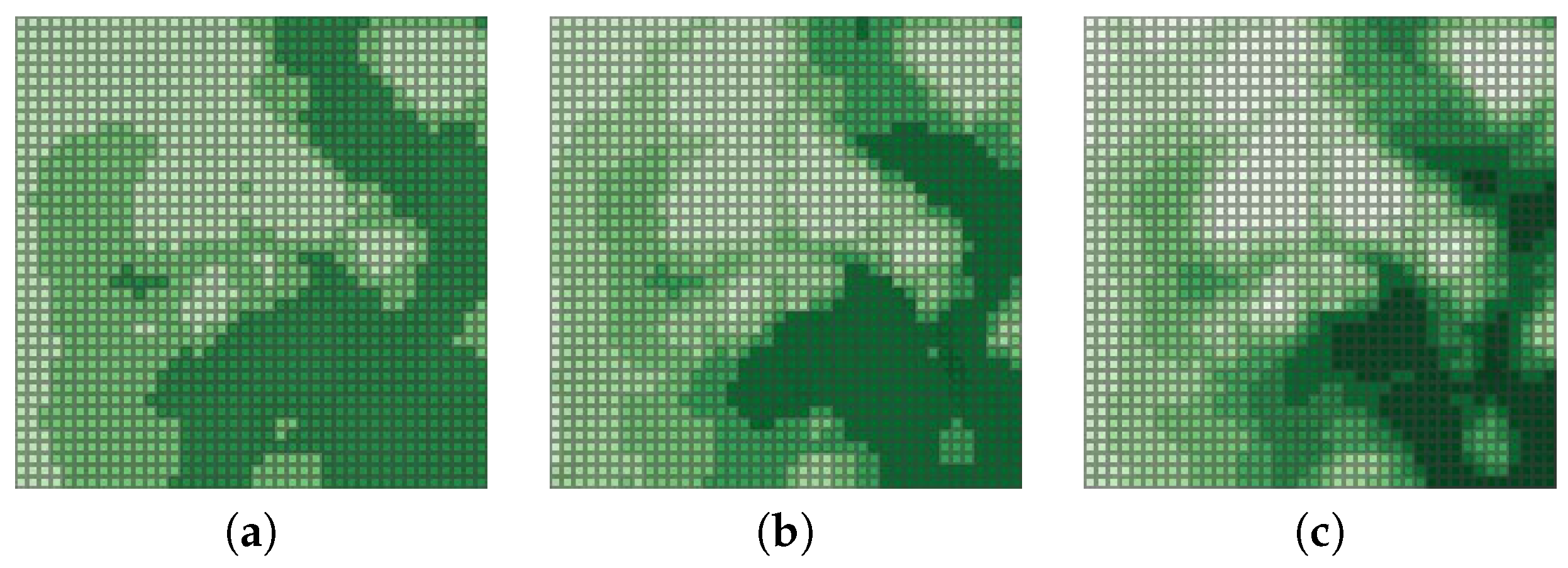
The stage after computation of depth maps is the classification of depth data. An approach like equal interval could possibly work if the system is sure to have plenty of fluid particles all around the map. This, however, is not the case for many applications that require tracking fluid translation. Thus, implementation of Jenks natural breaks method is helpful to provide a meaningful representation of the study area. As the spatial distribution of rain differs greatly for larger study areas, using natural breaks would allow us to visualize the data in a more appropriate way. The same is correct for visualizing terrain height as we cannot expect to have equally distributed height values within the map. The mapping engine considers three to nine different classes and therefore, by passing a parameter, various classification schemes can be evaluated and an appropriate one for the study area can be picked and utilized. Figure 5 shows varying classes of natural breaks used in representing the test area.
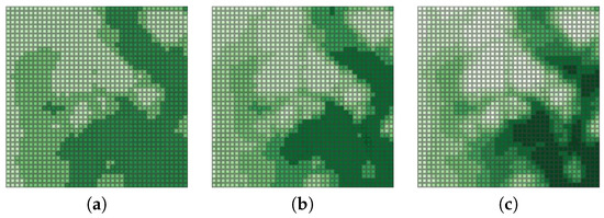
Figure 5.
Height map generated using (a) 4 classes, (b) 6 classes and (c) 9 classes.
Once the classes are organized through natural breaks method, the depth map is visualized. There are certain predefined color gradients that the system can receive as input. ColorBrewer [26] is used to export the color information and various schemes are predefined within the mapping engine. Since it is indicated as a bad method of representation [25], the rainbow color map is not included in the available color sets. The visualization can be viewed in real time or stored for later evaluation. Additionally, depending on the parameter received, the engine can capture snapshots of the study area in certain intervals. For example, the user can request to take snapshots every 5 simulation seconds for a total of 100 simulation seconds. This scenario provides us 20 snapshots stored in a file and later can be loaded to view the details of each snapshot.
5. Results and Discussion
The mapping engine was tested utilizing 10 different environments. Various terrain models were picked to utilize environments with differing characteristics. For each environment, height maps were generated and then a flood was simulated to keep track of water particles. Moreover, as previously discussed, cloud mechanics were randomly arranged to make the environment more dynamic. For each environment, a different number of clouds were generated, different animations were predefined and different rainfall intensities were selected.
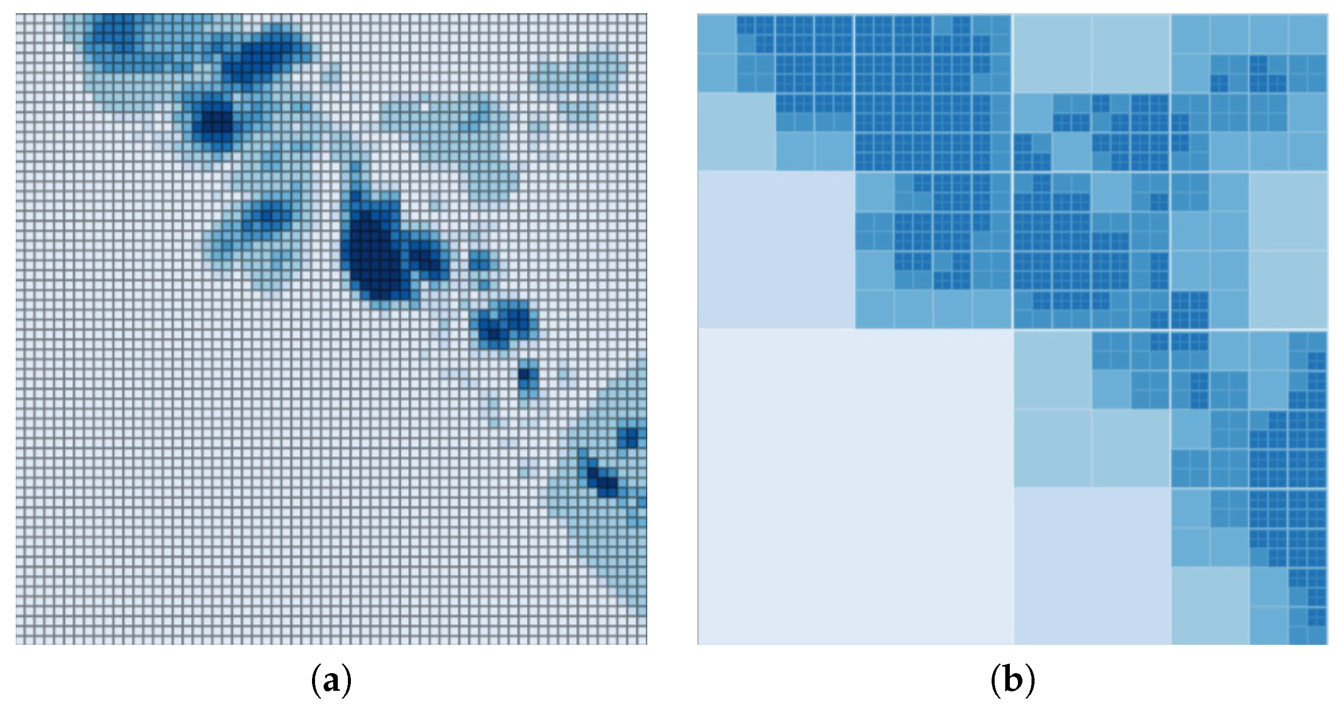
Considering the visuals generated by two approaches, it is apparent that regular grids with Jenks natural breaks for classification provide more in terms of depth. However, as the mapping engine processes more information with this approach, adaptive grids provide better performance. Figure 6, Figure 7 and Figure 8 show the differences in visualization of some our test environments.

Figure 6.
Visualization of the neighborhood flooding using (a) regular grids, (b) adaptive grids.
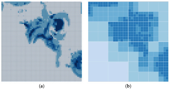
Figure 7.
Visualization of the canyon flooding using (a) regular grids, (b) adaptive grids.
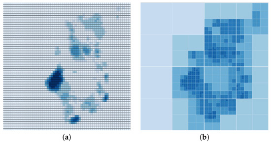
Figure 8.
Visualization of the mountain flooding using (a) regular grids, (b) adaptive grids.
According to these results, adaptive maps are not able to represent the study area as detailed as the regular approach if a depth limit is defined for the quadtrees. If the limit is lifted, it can describe the environment with better detail, yet the performance benefits are also cancelled and thus, it is not preferred. Moreover, it is challenging to set a hard particle limit on each node of the quadtree as the dynamic conditions of the environment are initially unknown. The mapping engine tries its best to estimate the depth limit and the particle limit using environmental parameters, such as maximum number of particles on the scene, terrain type, and terrain height variations.
Figure 7 illustrates one important issue regarding adaptive grids with limited depth. When a certain section of the environment has high depth values, the adaptive grid approach shows similar color in the surrounding cells due to compression. However, when we consider the regular grid approach with natural breaks classification, the local maxima are clearly represented. If an overall sense of depth is sufficient for the study, especially for larger areas like cities, then an adaptive approach may be preferred. For such a scenario, the focus of the study is to estimate larger sections of flooding within a city or neighborhood, rather than detecting pools of water formed around a single rock. As the details may not be necessary, performance benefits of adaptive grids can be utilized by the mapping engine.
On the other hand, Figure 8 shows that when local maxima are dispersed, unlike the previous scenario, then an adaptive approach does a better job describing classes of depth. Consequently, this is one of the factors that the mapping engine considers as it switches between different methods of representation. If there are similar values distributed over a large area, then the mapping engine prefers regular grids unless performance is a concern. On the other hand, when the depth values differ and there are few local maxima defined over the map, the adaptive approach is selected for representation unless more details are demanded.
As more rules are incorporated into the mapping engine, it yields better results in terms of the choices it is making. Several failures that occurred during the visualization tests were due to the lack of knowledge about the surroundings. In some cases, considering the affected area of the environment, the engine decided to increase the maximum depth of the quadtree, which actually caused frame-rate spikes. This is due to noisy terrains having more particle interaction. In such environments the computation takes longer and if the quadtree is too deep, it may perform worse than a regular grid. To fix such issues, additional rules are defined to guide the dynamic mapping engine to pick correct approaches.
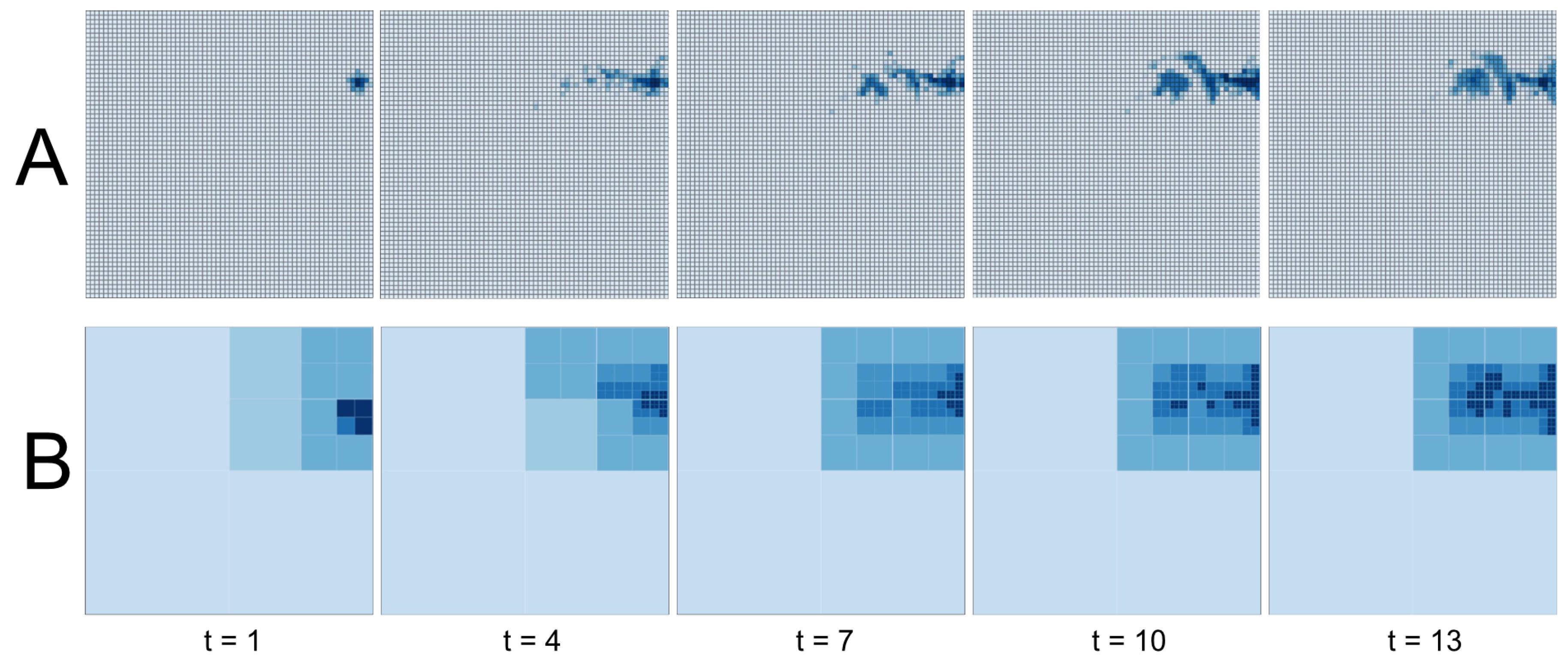
Figure 9 shows flood progression over 13 simulation seconds. When regular cells and adaptive cells are compared, several interesting results can be extracted. Firstly, as the flood is in its early stages, quadtree cannot represent the event properly due to lack of information. As the tree gets divided into four when number of particles passes beyond a certain limit, initial subdivision gives an incorrect sense of flooding for the upper right quarter of the study area. Then, as the particles spread around and the total number of particles on the scene increase, representation becomes more accurate. This is due to increased resolution due to additional subdivisions in the surrounding area. For this particular scenario, the dynamic mapping engine initially draws the map using the regular grid and then after 21 simulation seconds pass, it switches the representation to the adaptive grid.
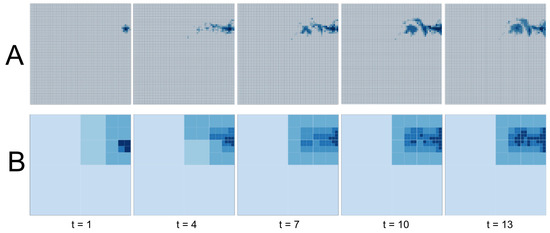
Figure 9.
Timeline of flooding using (A) regular grids, (B) adaptive grids.
Regular cells and quadtrees were utilized side-by-side to evaluate potential performance benefits of using adaptive cells. Table 1 shows several test environments and average refresh rate for each approach. After 50 runs on the same environments, capped at 300,000 and 400,000 particles, it is clear that adaptive cells improve performance. Consequently, the mapping engine optimizes the performance selecting adaptive cells as required. Nevertheless, if the performance is not a concern, the mapping engine can be instructed to optimize quality.

Table 1.
Performance comparison of regular grids and adaptive grids under different environmental conditions.
An important thing to remember is that the performance comparison is provided for the mapping engine only and not the simulation itself. Therefore, if the number of cells utilized by both approaches are the same, there should not be differences in performance. According to our tests, adaptive grid performs worse if depth limit is removed. Nevertheless, the dynamic mapping engine recognizes possible performance issues and therefore, it limits the depth of the quadtree.
6. Conclusions and Future Work
In this work, a flexible mapping engine, which can be used to visualize depth information for 3D Lagrangian simulations is presented to provide better insight for flooding scenarios. The engine having an adaptive resolution provides better efficiency than standard grid-based implementations. Making the choice to select the representation dynamically, shortcomings of both regular grids and adaptive grids are alleviated. Moreover, by utilizing position-based fluids as the underlying simulation method, advantages of position-based dynamics is acquired, which provides better simulation stability.
2D visualization of flooding utilizing adaptive spatial resolution is useful for multiple reasons. Firstly, earlier works of [21,24] provide insight about the benefits of utilizing 2D visualization alongside 3D as they underline that 2D representation is more maintainable and human-readable and therefore, it helps alleviate some of the complexities of 3D simulations. Moreover, through utilization of quadtrees and implementing the mechanism for the system to decide on which representation to choose, efficiency, as well as detail on demand are provided. Providing a depth mapping mechanism helps 3D Lagrangian simulations to describe particle clusters and hence, water levels in the case of flooding, more precisely.
Although the system is tested using several different environments, urban environments such as towns and cities present an additional challenge as the concept of water depth and terrain height must be considered in a different context. Even though the current implementation of the system considers the building, car, tree and similar entities separately, more testing needs to be performed to eliminate any potential inconsistencies regarding computation of depth and height. An interesting challenge would be to consider population to determine the risk factors of such flooding.
As underlined earlier, many of the environmental parameters are loaded through the component reader. These parameters are not altered after the initial processing. Simulating a fully dynamic environment with shifting wind direction over time, intensifying the rain, and considering soil erosion and soil absorption could yield interesting results. Such scenarios could be implemented end experimented with in the future.
Author Contributions
Conceptualization, I. Alihan Hadimlioglu and Scott A. King; methodology, validation, writing—original draft and visualization, I. Alihan Hadimlioglu; writing—review and editing, Scott A. King.
Funding
This research received no external funding.
Conflicts of Interest
The authors declare no conflict of interest.
References
- Herget, J.; Kapala, A.; Krell, M.; Rustemeier, E.; Simmer, C.; Wyss, A. The millennium flood of July 1342 revisited. Catena 2015, 130, 82–94. [Google Scholar] [CrossRef]
- Giordano, R.; Pagano, A.; Pluchinotta, I.; del Amo, R.O.; Hernandez, S.M.; Lafuente, E.S. Modelling the complexity of the network of interactions in flood emergency management: The Lorca flash flood case. Environ. Model. Softw. 2017, 95, 180–195. [Google Scholar] [CrossRef]
- Christodoulou, D.; Miao, S. Compressible Flow and Euler’s Equations: Volume 9 Surveys of Modern Mathematics; International Press: Somerville, MA, USA, 2014. [Google Scholar]
- Ladyzhenskaya, O.A. Mathematical analysis of Navier-Stokes equations for incompressible liquids. Annu. Rev. Fluid Mech. 1975, 7, 249–272. [Google Scholar] [CrossRef]
- Succi, S.; Yeomans, J.M. The Lattice Boltzmann equation for fluid dynamics and beyond. Phys. Today 2002, 55, 58–60. [Google Scholar]
- Gingold, R.A.; Monaghan, J.J. Smoothed particle hydrodynamics—Theory and application to non-spherical stars. Mon. Not. R. Astron. Soc. 1977, 181, 375–389. [Google Scholar] [CrossRef]
- Macklin, M.; Müller, M. Position based fluids. ACM Trans. Graph. 2013, 32, 104. [Google Scholar] [CrossRef]
- Alkemade, A.J.Q.; Nieuwstadt, F.T.M.; Groesen, E. The vorton method. Theory and applications to fluid mechanics. Appl. Sci. Res. 1993, 51, 153–158. [Google Scholar]
- Lucy, L.B. A numerical approach to the testing of the fission hypothesis. Astron. J. 1977, 82, 1013–1024. [Google Scholar] [CrossRef]
- Winchenbach, R.; Hochstetter, H.; Kolb, A. Constrained neighbor lists for SPH-based fluid simulations. In Proceedings of the ACM SIGGRAPH/Eurographics Symposium on Computer Animation (SCA’16), Zurich, Switzerland, 11–13 July 2016; Eurographics Association: Goslar, Germany, 2016; pp. 49–56. [Google Scholar]
- Teng, J.; Jakeman, A.; Vaze, J.; Croke, B.; Dutta, D.; Kim, S. Flood inundation modelling: A review of methods, recent advances and uncertainty analysis. Environ. Model. Softw. 2017, 90, 201–216. [Google Scholar] [CrossRef]
- Leskens, J.; Kehl, C.; Tutenel, T.; Kol, T.; de Haan, G.; Stelling, G.; Eisemann, E. An interactive simulation and visualization tool for flood analysis usable for practitioners. Mitig. Adapt. Strateg. Glob. Chang. 2015, 22, 1–18. [Google Scholar] [CrossRef] [PubMed]
- Liu, X.; Zhong, D.; Tong, D.; Zhou, Z.; Ao, X.; Li, W. Dynamic visualization of storm surge flood routing based on three-dimensional numerical simulation. J. Flood Risk Manag. 2016, 11, S729–S749. [Google Scholar] [CrossRef]
- Liu, J.; Gong, J.H.; Liang, J.M.; Li, Y.; Kang, L.C.; Song, L.L.; Shi, S.X. A quantitative method for storm surge vulnerability assessment—A case study of Weihai city. Int. J. Digit. Earth 2017, 10, 539–559. [Google Scholar] [CrossRef]
- Bender, J.; Finkenzeller, D.; Oel, P. HW3D: A tool for interactive real-time 3D visualization in GIS supported flood modelling. In Proceedings of the 17th International Conference on Computer Animation and Social Agents, Geneva, Swizerland, 7–9 July 2004; pp. 305–314. [Google Scholar]
- Luettich, R., Jr.; Westerink, J.J.; Scheffner, N.W. ADCIRC: An Advanced Three-Dimensional Circulation Model for Shelves, Coasts, and Estuaries. Report 1. Theory and Methodology of ADCIRC-2DDI and ADCIRC-3DL; Dredging Research Program Tech. Rep. DRP-92-6; U.S. Army Engineers Waterways Experiment Station: Vicksburg, MS, USA, 1992. [Google Scholar]
- Toros, H.; Kahraman, A.; Tilev-Tanriover, S.; Geertsema, G.; Cats, G. Simulating heavy precipitation with HARMONIE, HIRLAM and WRF-ARW: A flash flood case study in Istanbul, Turkey. Eur. J. Sci. Technol. 2018, 13, 1–12. [Google Scholar] [CrossRef]
- Bao, Y.; Huang, Y.; Liu, G.R.; Zeng, W. SPH simulation of high-volume rapid landslides triggered by earthquakes based on a unified constitutive model. part ii: Solid-liquid-like phase transition and flow-like landslides. Int. J. Comput. Methods 2018, 1850149. [Google Scholar] [CrossRef]
- Zhang, S.; Xia, Z.; Wang, T. A real-time interactive simulation framework for watershed decision making using numerical models and virtual environment. J. Hydrol. 2013, 493, 95–104. [Google Scholar] [CrossRef]
- Macchione, F.; Costabile, P.; Costanzo, C.; Santis, R.D. Moving to 3-D flood hazard maps for enhancing risk communication. Environ. Model. Softw. 2019, 111, 510–522. [Google Scholar] [CrossRef]
- Van Ackere, S.; Glas, H.; Beullens, J.; Deruyter, G.; Wulf, A.; De Maeyer, P. Development of a 3D dynamic flood WEB GIS visualisation tool. Int. J. Saf. Secur. Eng. 2016, 6, 560–569. [Google Scholar] [CrossRef]
- Ghazali, J.N.; Kamsin, A. A real time simulation of flood hazard. In Proceedings of the 2008 Fifth International Conference on Computer Graphics, Imaging and Visualisation, Penang, Malaysia, 26–28 August 2008; pp. 393–397. [Google Scholar]
- Adda, P.; Mioc, D.; Anton, F.; McGillivray, E.; Morton, A.; Fraser, D. 3D flood-risk models of government infrastructure. Int. Arch. Photogramm. Remote Sens. Spat. Inf. Sci. ISPRS Arch. 2010, 38, 6–11. [Google Scholar]
- Alahmed, S.; Zou, Q. Modelling urban coastal flooding through 2-D array of buildings using smoothed particle hydrodynamics. In Proceedings of the 35th International Conference on Coastal Engineering, Antalya, Turkey, 17–20 November 2016. [Google Scholar]
- Liu, Y.; Heer, J. Somewhere over the rainbow: An empirical assessment of quantitative colormaps. In Proceedings of the ACM Human Factors in Computing Systems (CHI), Montreal, QC, Canada, 21–26 April 2018; pp. 1–12. [Google Scholar]
- Harrower, M.; Brewer, C.A. ColorBrewer.org: An online tool for selecting colour schemes for maps. Cartogr. J. 2003, 40, 27–37. [Google Scholar] [CrossRef]


© 2019 by the authors. Licensee MDPI, Basel, Switzerland. This article is an open access article distributed under the terms and conditions of the Creative Commons Attribution (CC BY) license (http://creativecommons.org/licenses/by/4.0/).