Abstract
Remote sensing has been widely used in vegetation cover research but is rarely used for intercropping area monitoring. To investigate the efficiency of Chinese Gaofen satellite imagery, in this study the GF-1 and GF-2 of Moyu County south of the Tarim Basin were studied. Based on Chinese GF-1 and GF-2 satellite imagery features, this study has developed a comprehensive feature extraction and intercropping classification scheme. Textural features derived from a Gray level co-occurrence matrix (GLCM) and vegetation features derived from multi-temporal GF-1 and GF-2 satellites were introduced and combined into three different groups. The rotation forest method was then adopted based on a Support Vector Machine (RoF-SVM), which offers the advantage of using an SVM algorithm and that boosts the diversity of individual base classifiers by a rotation forest. The combined spectral-textural-multitemporal features achieved the best classification result. The results were compared with those of the maximum likelihood classifier, support vector machine and random forest method. It is shown that the RoF-SVM algorithm for the combined spectral-textural-multitemporal features can effectively classify an intercropping area (overall accuracy of 86.87% and kappa coefficient of 0.78), and the classification result effectively eliminated salt and pepper noise. Furthermore, the GF-1 and GF-2 satellite images combined with spectral, textural, and multi-temporal features can provide sufficient information on vegetation cover located in an extremely complex and diverse intercropping area.
1. Introduction
Increasing food production to meet the enormous demand for food due to the world’s population growth has become a widespread concern [1,2]. Intercropping serves as an excellent means to increase food productivity, enhancing farm income, improving soil and water quality, and reducing greenhouse gas emissions [3]. Intercropping not only plays an important role in both land resource management and food production solutions but also supports dynamic interactions between trees and crops [4]. Intercropping has been often used and has become essential to the world’s agricultural production. Many studies showed that reasonable intercropping can efficiently utilize natural resources (e.g., light, heat, fertilizer, and water), reduce risks of nature disasters, reduce weed competition, and improve yields of limited cultivated land. On the other hand, inappropriate intercropping patterns may have adverse effects, such as decreasing production and ecological deterioration [4]. Therefore, surveying and mapping plant types, quantity structures, and spatial distribution characteristics are important in improving intercropping systems and in estimating potential yields and tree crop system adjustments.
Remote sensing has been widely used in monitoring cropping at different spatial and temporal scales [5]. However, intercropping has been rarely addressed with remote sensing in the literature [6]. Compared with conventional planting patterns, intercropping is challenging in remote sensing monitoring due to the complexities of spatial distributions. First, when several crops are planted together during the growing season, different crops may have spectral intersections at different growth stages. Under such conditions, discriminating different intercropping objects from a single image is relatively difficult. High temporal resolution remote sensing has been used in crop monitoring, and it has been proven that time-series images can perform better than single-data mapping methods [7,8]. Belgiu et al. classified various crops of Sentinel-2 time-series images using a time-weighted dynamic time warping method to three different test areas in Romania, Italy, and the USA with high levels of overall accuracy [9]. Second, in an intercropping area, differences in the sizes and shapes of tree canopies lead to uncertainty at canopy edges and to different spectral crop characteristics under tree canopies. Crops and trees are inlaid and intertwined in space, creating some forms that are difficult to distinguish and extract. Studies have generally used high-resolution remote sensing imagery to extract trees. Hartfield et al. [10] described a novel Cubist-based approach to modelling woody cover in Oklahoma and Texas using 1 and 2 m spatial resolution data. D. S. Culvenor [11] applied tree identification and delineation algorithms to delineate tree crowns of a Mountain Ash forest from 0.8 m resolution imagery. Mayossa et al. [12] introduced a semi-automatic classification method based on a QuickBird texture analysis to differentiate coconut palms from oil palms in Melanesia. In tree–crop monitoring, high spatial remote sensing imagery must be used.
In this work, images captured by GF-1 and GF-2, two of the satellites used in China’s high-resolution Earth Observation System, are employed. The data can be downloaded from the China Resource Satellite Center [13]. The GF-1 satellite includes two panchromatic multispectral sensors (PMS) and four wide field view (WFV) cameras, which can acquire data at a high spatial resolution, with broad coverage, and at a high revisit frequency (The revisit frequency of the GF-1 PMS is four days and that of the WFV cameras is two days) [14]. Each PMS includes a panchromatic band (0.45–0.90 μm) of 2 m resolution and multispectral bands of 8 m resolution as follows: blue band (0.45–0.52 μm), green band (0.52–0.59 μm), red band (0.63–0.69 μm), and Near-InfraRed (NIR) band (0.77–0.89 μm) [15]. The revisit frequency of the PMS aboard the GF-2 satellite is 5 days, providing a panchromatic band of 0.81 m resolution and multispectral bands (B, G, R, and NIR) of 3.24 m resolution. Compared to IKNOS, Worldview, Quickbird, and SPOT 6/7 images, GF images are favorable. Of these sub-meter resolution remote sensing data, Worldview and Quickbird images are more expensive than IKNOS images whereas the price of a GF-2 image per km2 is less than one seventh of the price of an IKNOS image (0.82 m panchromatic and 4 m multispectral bands: R, G, B, and NIR). GF satellites can provide very high spatial resolution, low-cost, and continuous data for agricultural and forestry monitoring. GF-1 has been used to study land cover [16], but few studies have used GF-1 or GF-2 to monitor cropping.
Many machine learning algorithms have been applied for crop classification, such as maximum likelihood classification (MLC), neural network, Support Vector Machine (SVM), and Random Forest (RF) [17]. The SVM and RF have been shown to outperform the MLC in classifying crops [18,19]. Rodriguez et al. [20] proposed a Rotation Forest (RoF) and performed experiments using 33 data sets from the University of California Irvine Machine Learning Repository. The results of those studies showed that the RoF performed better than three ensemble learning methods (Bagging, AdaBoost and RF methods) [20]. The RoF is an ensemble approach based on feature transformation and the segmentation of attribute sets [20]. The RoF adopts a principal component analysis (PCA) of feature subtests to reconstruct full feature space and to improve the diversity of all base classifiers, distinguishing it from the RF. Moreover, the RoF has been used for optical and Fully Polarimetric Synthetic Aperture Radar remote sensing classification, and it has been demonstrated that the RoF achieves a higher level of classification accuracy than the RF [21,22].
However, regardless of the many types of classification methods available, each method presents its own advantages and weaknesses [23]. For instance, the SVM is highly accurate but offers a slow processing speed [24]. Although the MLC is less accurate, it is still widely used for image classification due to its rapid calculation capabilities and convenient implementation. Balancing the trade-off between accuracy and speed is crucial. The use of ensemble learning methods to increase classification accuracy has received much attention [25].
This paper used the SVM as the base classifier of the RoF method. This method has been used as a network composed method for anomaly detection [26] that (i) can increase the diversity of base classifiers, (ii) is suitable for small samples and high-dimensional classification objects, and (iii) effectively prevents overfitting.
Based on Chinese GF-1 and GF-2 satellite imagery features, this study has developed a comprehensive feature extraction and intercropping classification scheme. The experiments have shown that GF-1 and GF-2 satellite images combine spectral, textural and multi-temporal features to provide sufficient vegetation coverage information for extracting crop information from extremely complex and diverse intercropping regions. This study serves as a basis for the application of Chinese GF satellites for the monitoring of intercropping in areas such as precision agriculture and forestry.
2. Study Area and Data
2.1. Study Area
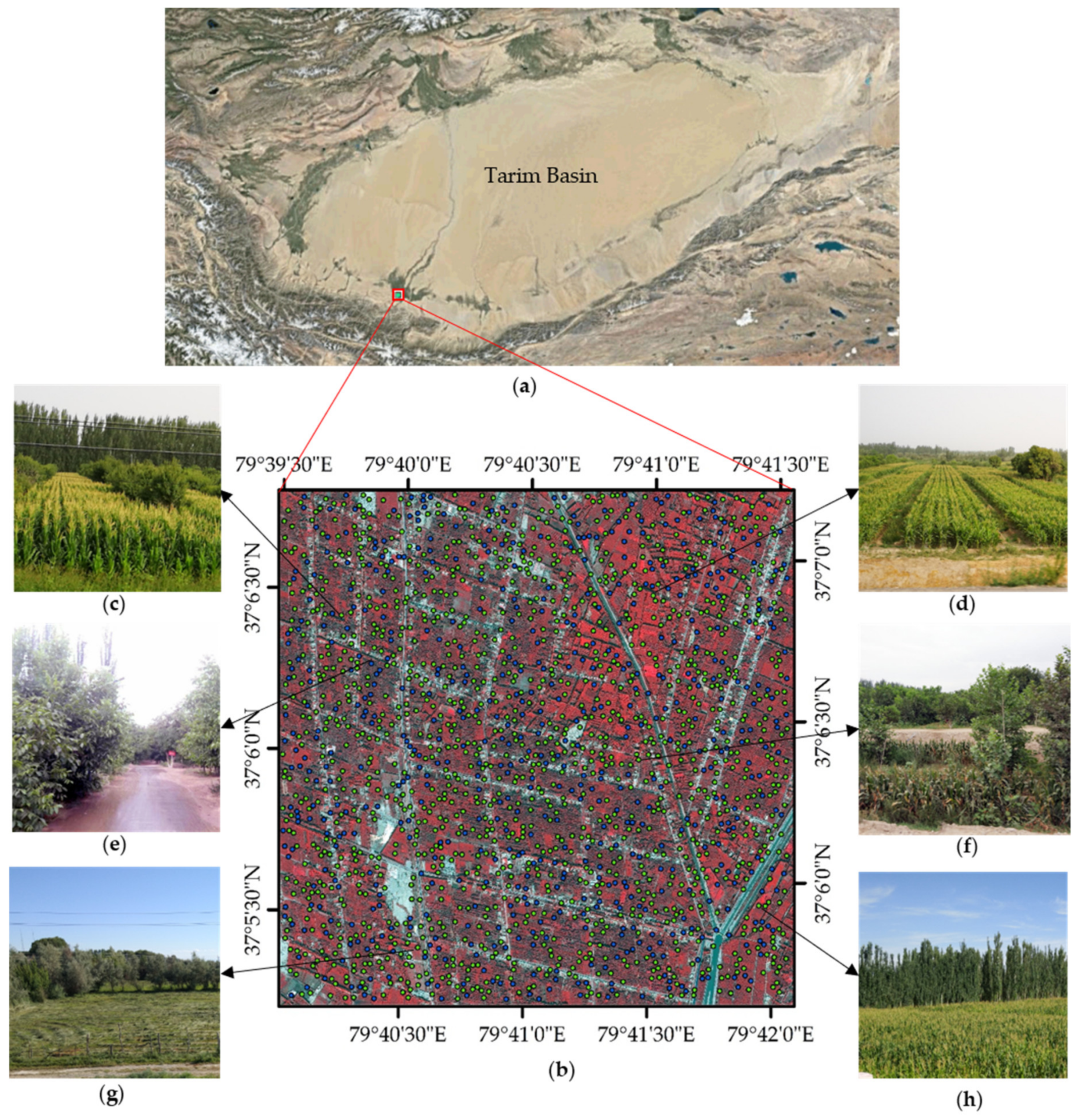
The selected study area is located in Moyu County, Hetian, Tarim Basin. The Tarim Basin is located in southern Xinjiang. The area covers the southern Tianshan Mountains, the northern Kunlun Mountains, and the hinterland of the Taklimakan Desert. Foothills close to the basin are composed of alluvial plains formed by seasonal snowmelt, forming a well-known forest fruit producing area. The area is characterized by a warm temperate dry desert climate and is a typical arid oasis agricultural area. The area lacks water resources but supports a large population and per capita arable land area of less than 2 acres. To increase local farmer incomes, the intercropping of fruit trees and crops has been promoted since the end of the last century. Horticultural activities that characterize the Tarim Basin benefit from the interplanting model. The industrial forest fruit of the region accounts for 83.47% of the forest fruit area of Xinjiang, and local fruit production accounts for 67.36% of that of Xinjiang [27]. More than 80% of local counties include intercropping areas. Therefore, the selection of the study areas in the Tarim Basin is representative.
The area is a typical rotation and intercropping area. The main trees produced are walnut trees, and the main crops grown are winter wheat and maize. A shelterbelt dominated by populus bolleana is also planted. This planting mode has the effect of sand fixation and storm resistance and increases the yields of economic crops while producing grain. The region has become a new planting model for oasis agriculture. The selected test area is 3.1 × 3.1 km, covering an area of 961 ha, but it includes almost all features of typical agricultural planting areas in arid areas: shelter forests, economic trees, crop rotation systems (wheat-maize), residential areas, roads, water systems, sandy areas, and grassland. In particular, the spatial structure of intercropping areas is extremely complex and diverse. Walnut trees and different crops (wheat, vegetables, grassland and maize) are intercropped with completely different row spacing and densities (as shown in (c–h) of Figure 1), creating complex spatial distribution characteristics. Therefore, the test area serves as an ideal sample area for intercropping classification tests.

Figure 1.
Map showing the study area: (a) study area in the Tarim Basin; (b) study area illustrated with false colour combinations (near-infrared, red, and green bands) for September 18, 2016. The green points denote training samples and the blue points denote validation samples.
2.2. Field Sampling
For the vegetation classification, seven land cover categories were classified, including walnut trees, maize, shelterbelts, grassland, vegetable cropland, water, and bare ground. The bare ground area includes all non-vegetated areas such as residential areas, roads, and sandy areas. A total of 1963 samples were selected for manual field surveys (July to August 2016) by the visual interpretation of different land cover types as shown in (b) of Figure 1. All samples are shown in pixels divided into two groups: 1363 samples (64 061 m2) were used as training data (green points in (b) of Figure 1) for the development of a classification algorithm and the remaining 600 samples (15,250 m2) were used as validation data (blue points in (b) of Figure 1) to evaluate the classifier.
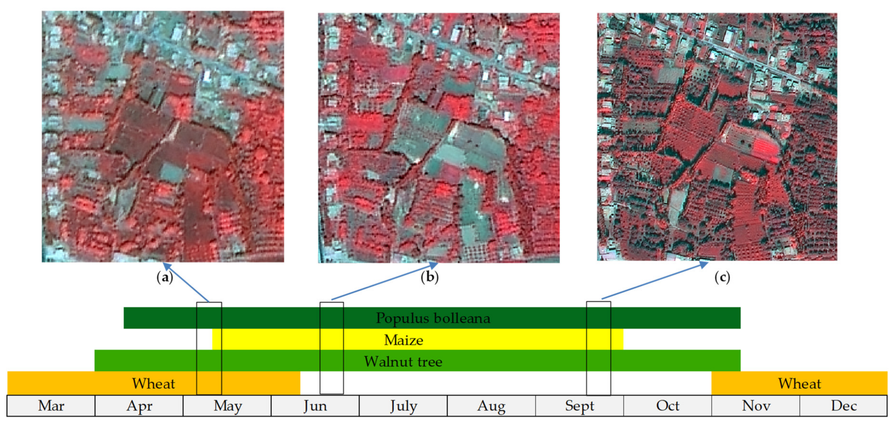
Previous studies showed that the area has a double cropping form. Winter wheat is planted at the end of October every year, and the area enters a greening period in the middle of March of the next year. Wheat ears grow in May when the Normalized Difference Vegetation Index (NDVI) reaches its peak, and harvesting begins in early June. Summer maize is planted in June, seedlings emerge at the end of June, and crops reach advanced vegetative phases in September [28]. Data from field observation sites and surveys of local farmers show the growth period of main crops in the study area as illustrated in Figure 2. According to surveys of local farmers, the harvesting and sowing periods of regional crops usually varies within ten days. Three temporal images with no cloud coverage in the test area were selected from GF-1 PMS1 on May 10, 2016, from GF-1 PMS2 on June 24, 2016, and from GF-2 PMS2 on September 18, 2016. Crop growth patterns corresponding to each remote sensing image shown in Figure 2a–c were randomly selected for the same farmland area from three images, revealing differences observed between crops and trees. These images provide crop rotation and growth information, reflecting differences observed between some crops and trees.
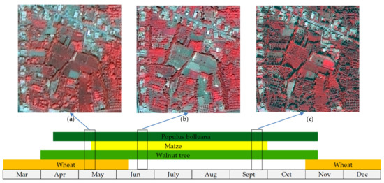
Figure 2.
Growth period and sample images of study area; (a) Sample GF-1 images acquired on May 10; (b) Sample GF-1 image acquired on 2 June 24, 2016; (c) Sample GF-2 image acquired on September 18, 2016.
2.3. Remote Sensing Data Pre-processing
All GF-1 and GF-2 images were preprocessed in ENVI 5.3.1, which applies ortho-rectification, radiometric calibration, atmospheric correction, the fusion of panchromatic and multispectral bands, and geometric registration. The three images were projected in Albers Conical Equal Area coordinate system World Geodetic System 1984 to obtain the planting area. Orthophoto-rectification was applied to the Rational Polynomial Coefficient (RPC) parameters of the image and to the GMTED2010 digital elevation model (DEM) in ENVI. Radiation calibration involves converting the originally recorded digital number (DN) into the reflectivity of the outer surface of the atmosphere. The parameters of the satellite sensors are shown in Table 1; all the parameters have been input into the Radiometric Calibration tool of ENVI for radiation calibration. The ground elevation of the area is set to 1.2 km, and since the latitude of the area is 37° N, the atmospheric model of the GF-1 image for May 10, 2016, is set to the Sub-Arctic Summer, and the GF-1 image for June 24, 2016, and GF-2 image for September 18, 2016, are set to the Mid-Latitude Summer. The atmospheric correction converts radiance or surface reflectance into the actual reflectance of the surface to eliminate errors resulting from atmospheric scattering, absorption, and reflection. The atmospheric correction algorithm used in ENVI 5.3.1 is the FLAASH Atmospheric Correction module developed from the MODTRAN5 radiation transmission model.

Table 1.
Absolute radiometric calibration coefficients of GF-1 and GF-2 images used in this work.
In recent decades, a variety of hyperspectral image and multispectral image fusion algorithms have been proposed [29,30,31,32,33], proving that a fusion image can effectively improve the accuracy of land cover classification and vegetation detection results [34,35]. Since GF-1 and GF-2 have different panchromatic-multispectral spatial resolutions, they must be fused to generate high-resolution multispectral images. The Gram-Schmidt Pan Sharpening method is one of the most popular algorithms used to pan-sharpen multispectral imagery. This method outperforms most other pan-sharpening methods in both maximizing image sharpness and minimizing colour distortion [36]. In this study, for GF-1 and GF-2 PMS images, new synthetic images are generated with the Gram-Schmidt Pan Sharpening method to fuse the panchromatic band with multispectral bands.
3. Methodology
3.1. Feature Selection
After pre-processing, multispectral images of GF-2 at 1 m resolution and of GF-1 at 2 m resolution were generated. In the GF-2 image, textural features of different ground objects are clearer and more effective; thus, the spectral and textural features of GF-2 are used. As described in Section 2.2, there are visible differences in crop growth across the three images. The spectral features of the other two temporal GF-1 images are introduced to explore the accuracy of using multi-temporal images in the intercropping classification to increase the characteristic differences in various crops for the growing period.
Various vegetation indices have been referenced in other works [18], among which few have been commendably validated. For the present study, the NDVI and Enhanced Vegetation Index (EVI) were used.
The NDVI is one of the most widely used vegetation indices for studying vegetation phenology [37]. The NDVI limits spectral noise caused by certain illumination conditions, topographic variations and cloud shadows [38,39] to reveal the growth state and spatial distribution density of vegetation and separate vegetation from water, buildings, and bare ground [37]. The third and fourth bands of the GF-2 and GF-1 images are used to calculate the NDVI separately at 1 and 2 m resolutions as shown in Equation (1) [39]. denotes the reflectance of the k-th band.
The EVI offers advantages when applied to densely vegetated areas. The effects of soil backgrounds and aerosol scattering were corrected by adding a blue band (the first bands of GF-1 and GF-2) to enhance vegetation signals, to improve sensitivity to high biomass regions while minimizing soil and atmospheric effects [40] and to compensate for deficiencies of an easily saturated NDVI [41]. In the GF-2 image for September 18 used in this study, almost all crops were in a period of high NDVI values. Therefore, the EVI features of three different phases are adopted with the calculation shown in Equation (2) [42] as follows:
The NDVI and EVI calculated from GF-1 should be resized to a 1 m resolution to perform the classification algorithm.
A Gray level co-occurrence matrix (GLCM) is often used to extract textural features [19]. The GLCM is obtained by calculating the second-order combined conditional probability density of greyscales, which are used to describe the spatial distribution (direction and adjacent intervals) and structural features (arrangement rules) of greyscales of each pixel. The GLCM method has been widely used for texture analyses and pattern recognition and plays a central role in improving the accuracy of image segmentation and classification in remote sensing [43]. Wang et al. used the GLCM and different spectral features for worldview-3 for the mapping of mangrove trees, which improved the accuracy [44]. Lan et al. proved that using appropriate parameters for the scale of GLCM texture windows can effectively improve the classification accuracy of geographical analyses of optical remote sensing images [45]. GLCM-derived features are sensitive to texture boundaries. In intercropping areas, the shapes and heights of crops and trees are significantly different. Walnut trees and populus bolleana have different tree spacing features; according to field observations and a previous study, walnut trees are usually spaced more than three meters apart [28] while poplars in shelter forests are very dense at usually 4~6 trees per square meter. The “Co-occurrence Measures” tools of ENVI 5.3.1 were used to extract the GLCM at different window sizes, including the mean value, variance, homogeneity, contrast, dissimilarity, entropy, second moment, and correlation. These texture measures can be divided into four categories: features based on information theory, features based on statistical characteristics, features based on linear relationships, and features that express clarity. The window size was set to 5 × 5 in this study according to comparative experiments. In total, 32 texture feature bands were obtained from the GF-2 image.
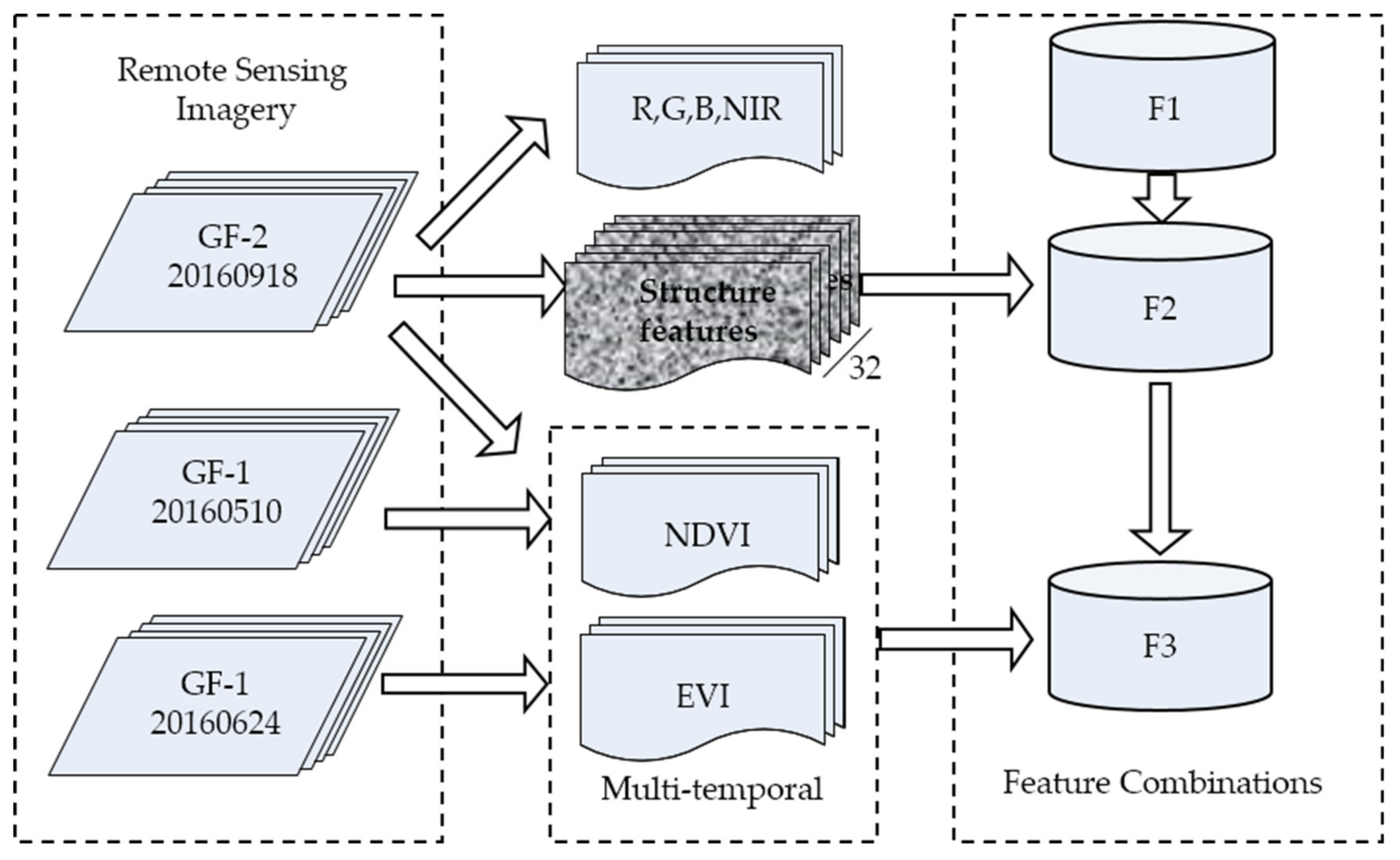
To explore the feature combination method, all features have been combined into three groups as follows:
- F1. Spectral features of GF-2 images, which include fused multi-spectral GF-2 images (features 1–4 in Table 2).
Table 2. Features of the combinations.
- F2. Multisource information of GF-2 images, including F-1 and textural features (features 1–36 in Table 2).
- F3. Multi-temporal and multisource information, including the F2 and GF1 NDVI, EVI GF2 NDVI, and EVI (features 1–42 in Table 2).
The pre-processing and feature combination workflow is shown in Figure 3.
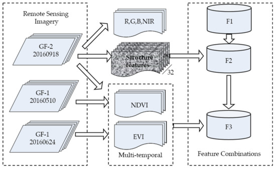
Figure 3.
Workflow for feature selection.
3.2. Intercropping Classification
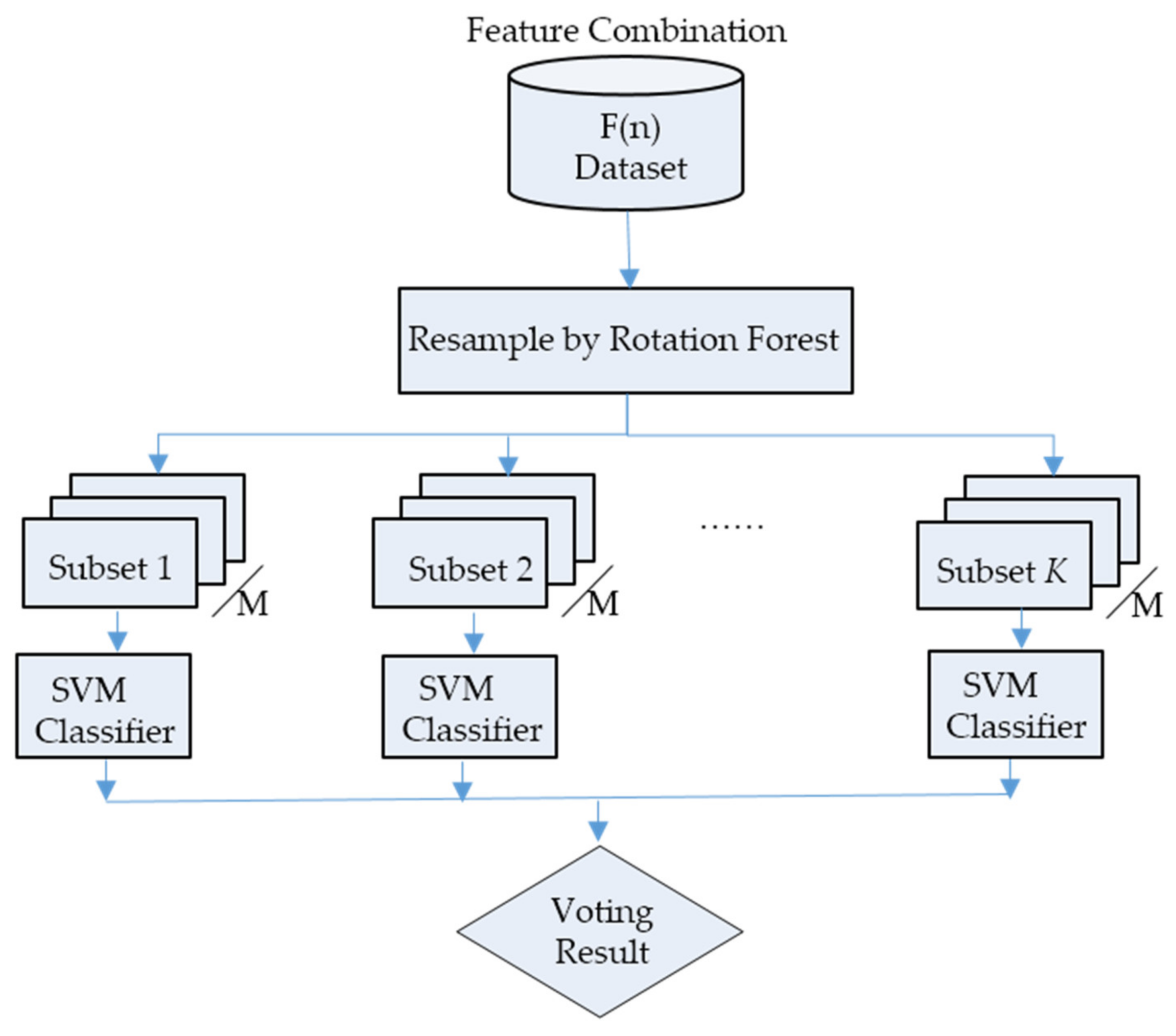
In this work, we applied the RoF using SVMs as base classifiers (RoF-SVM) for intercrop classification. First, it uniformly divides the feature set into subsets at random [21]. Then, the subsets are transformed to obtain new samples through reconstructing and are then used to train the base classifiers to increase the differences between them to generate diverse and accurate base classifiers [46]. In this study, the proposed ensemble learning method also increased the level of diversity between base feature transformations and the segmentation of attribute sets. However, the result obtained from the RoF-SVM was different from that of the ordinary RoF using decision trees as base classifiers. The SVM is used as a base classifier, as it better solves the high-dimensional small sample non-linear problems. Figure 4 illustrates the workflow.
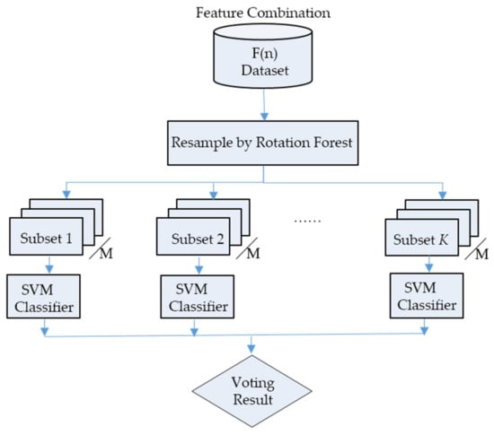
Figure 4.
RoF-SVM classification flowchart.
Let be the training dataset, which is an matrix. represents the number of training objects, and represents the number of features. Let denote the vector with class labels in training set where takes a value of the set of class labels and where denotes the number of classes. Let denote the feature set and let denote the number of subsets of features after splitting. Let be the number of base classifiers in the ensemble, and let be the base classifiers. The rotating forest model is built as follows:
- Input the initial sample set , which includes n features, and the number of base classifiers L.
- Randomly divide into equally sized subsets: where features were obtained from each subset. When the number of features is not divisible, the remaining features are added to the last subset of features.
- Process subsets as follows:
- 1)
- Let be the -th subset of features used to train the -th classifier, . Let be the sample set with only features involved in subset . This subset can be viewed as a reduced-dimension dataset of original set and thus as an matrix where is the number of features in subset . Then, apply the bootstrap method is to to obtain new sample subset .
- 2)
- Perform a principal component analysis (PCA) of to calculate coefficients of the principal components.
- 3)
- Repeat Steps 1 and 2 and organize the obtained principal component coefficients into a matrix :
- 4)
- Rearrange to obtain rotation matrix and generate new sample set = .
- 5)
- Select as the base classifier (SVM is adopted in this study) to obtain an ensemble classifier () and then return to Step 2, loop times, and obtain the ensemble classifier [20].
- 6)
- Let be the sample to be classified and is the probability of classifier determining that sample belongs to the -th class. Then, the credibility of the sample assigned to a certain category is defined as Equation (4), which is adapted from [20]:Again, is the number of base classifiers, and is the number of categories (classes). Sample belongs to the category of maximal reliability.
4. Results and Analysis
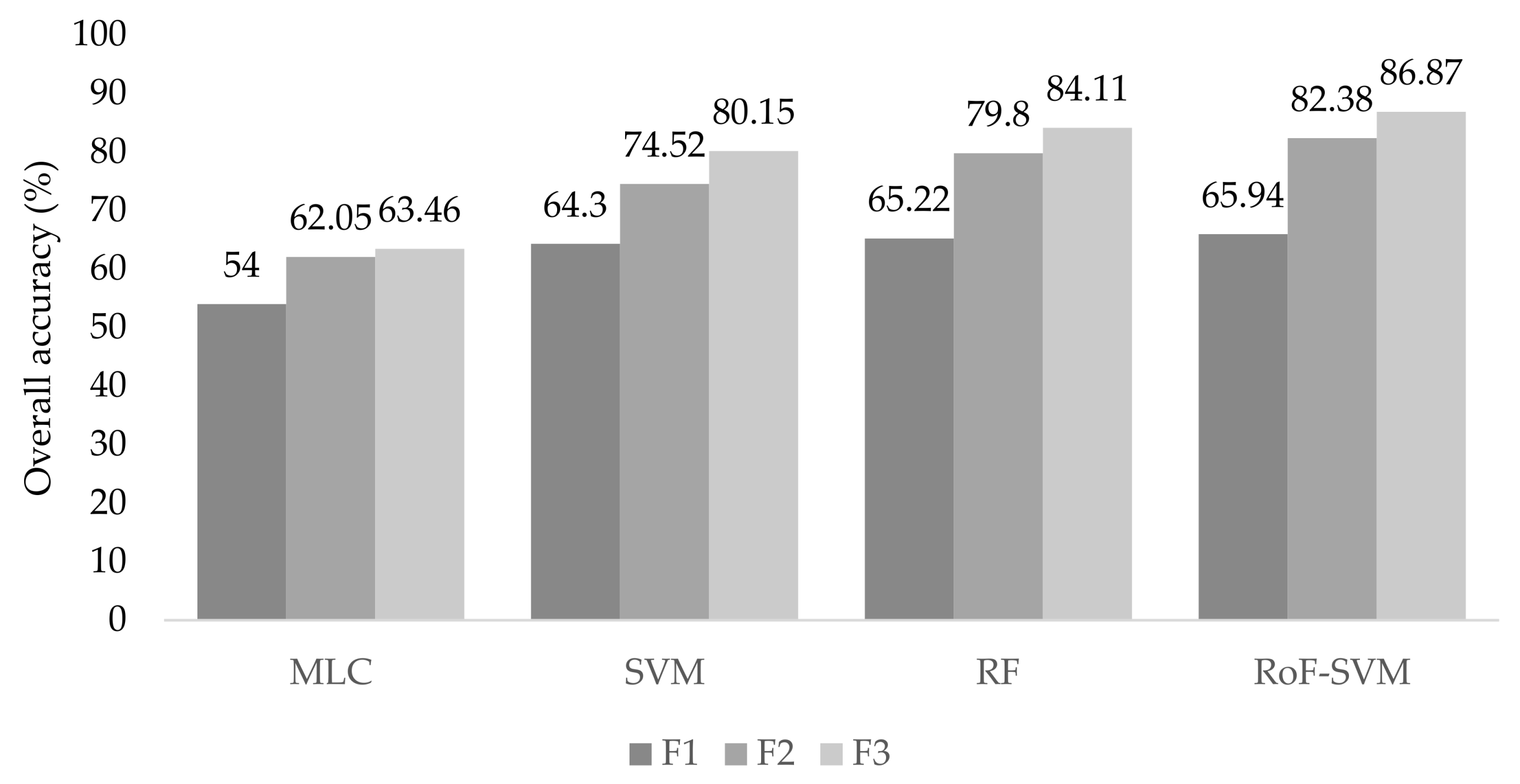
In this section, the parameter values of the RoF-SVM algorithm are initially determined. Then, to evaluate the impact of multi-feature and multi-temporal data on classifications, the RoF-SVM is adopted to classify the three different feature combinations presented in Section 3.1. The optimal feature combination is selected based on the accuracy of classification results. Then, to evaluate the effectiveness of the RoF-SVM, classification experiments are performed by applying the MLC, SVM and RF classification methods to the same training samples and input feature combinations. The overall accuracy (OA) is used to compare the results of different feature combinations of all classification methods. The best classification results for each classification method are then compared in terms of OA, manufacturer accuracy, user accuracy indicators, and kappa coefficients to evaluate the performance of different classifiers.
4.1. RoF Parameter Setting
The RoF-SVM ensemble method is applied to each dataset using the Radial Basis Function (RBF) as the kernel function. A 10-fold cross-validation is used to determine the factor of the gamma and cost of the SVM. The RoF uses two parameters that influence the accuracy of its results: the number of subsets, , and the number of base classifiers in the ensemble, . For the three feature combination groups, the value of is set to 6, and experiments are conducted using where is the total number of features. The OAs using the three feature combinations listed above, F1, F2 and F3, are shown in Figure 5. The three combinations indicate that the accuracy levels are extremely low when , and thus no partitioning of features is performed. The OA increases along with an increase in but tends to be stable when reaches a certain value. In F1, the combination group has only four features, and tends to be stable. F2 has 36 characteristic dimensions, and generates the highest OA. In F3, with 42 characteristic dimensions, when , the accuracy level is the highest of all combinations.

Figure 5.
Overall accuracy (%) with respect to the number of subsets K.
In groups F1, F2 and F3, optimal values are 3, 12, and 14, respectively. We then fix the optimal values and conduct experiments using instances of RoF-SVM constructed with different numbers of base classifiers, . The OA values of the RoF-SVMs of different sizes are shown in Figure 6. The OA increases when the size of the ensemble increases from 2 to 10 but converges when the value is not less than 10.
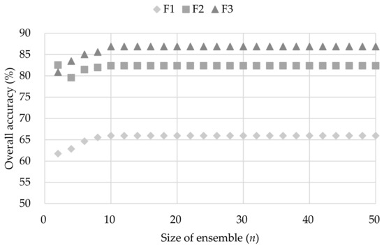
Figure 6.
Overall accuracy (%) versus ensemble size (n).
4.2. Comparison of Different Feature Combinations
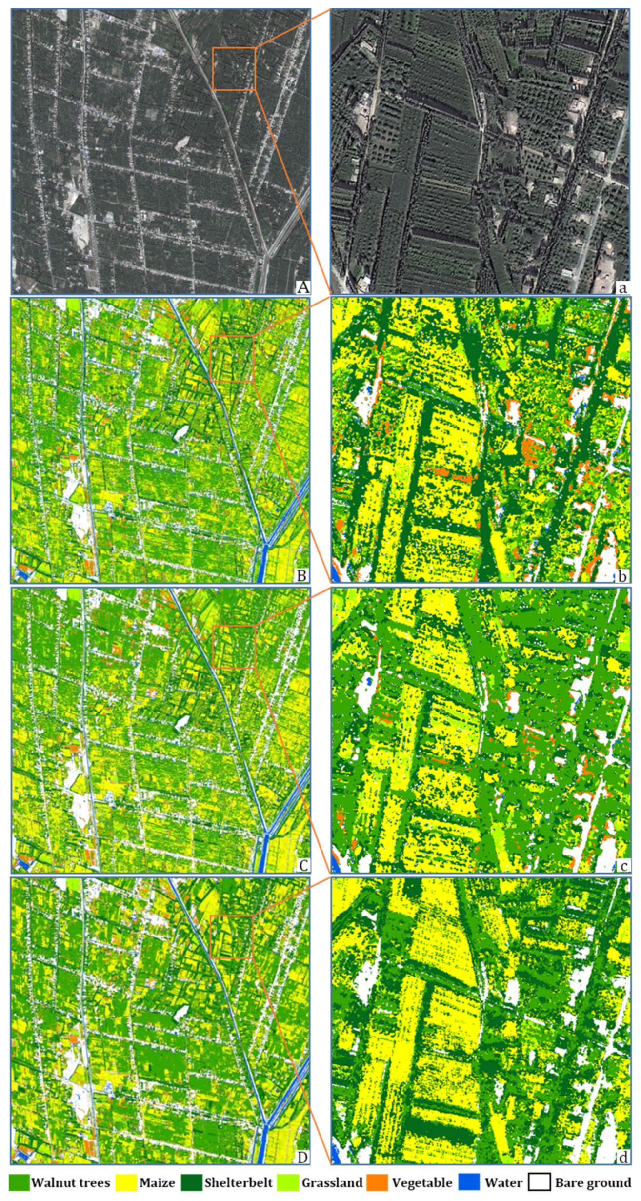
The experiments presented in Section 4.1 reveal that the optimal combination of and for each group is as follows: and with the highest OA (65.94%) for the best result of the F1 combination. For the F2 combination, and generate the highest OA (82.38%) and the best result of the F1 and F2 combinations. For the F3 group, and generate the best result of the three combinations (OA = 86.87%). Classification results of the RoF-SVM for the three groups are shown in Figure 7 and Table 3.
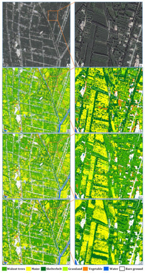
Figure 7.
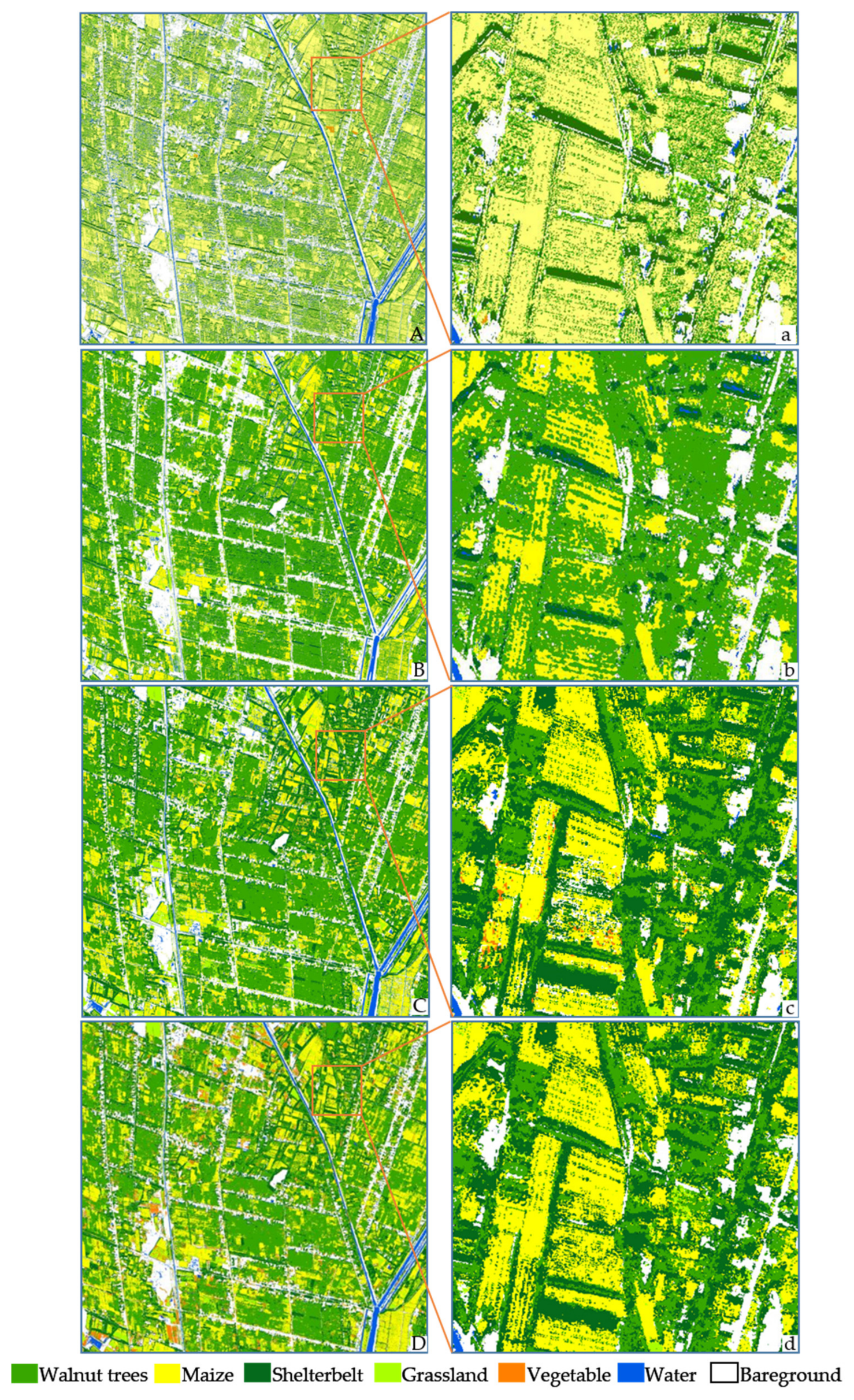
Crop classification maps based on the RoF-SVM: (A) True colour map of GF-2; (a) Sample area of (A); (B) RoF-SVM classification results of F1; (b) Sample area of (B); (C) RoF-SVM classification results of F-2; (c) Sample area of (C); (D) RoF-SVM classification results of F3; (d) Sample area of (D).
Table 3.
Image Classification Accuracy Levels of the RoF-SVM for three Combinations.
The F1 group containing only GF-2 multispectral bands is evidently less accurate than the other two combinations. When combined with spectral and texture features based on the GF-2, F2 improved the OA by 16.44%, and the kappa coefficients increased by 0.12. Evidently, water can be most easily distinguished. The additional texture features derived from the GLCM remarkably improve all forms of vegetation classification accuracy. A marked increase is observed in the distinction of walnut trees and crops. However, for different crops of the growing season, lush grassland is confused with vegetables and walnut trees are confused with shelterbelts. The classification results of F2 still present a relatively large degree of error. F3 combined multi-temporal NDVI and EVI features based on F2. The classification maps and accuracy levels show a significant improvement in the discrimination of different crops. Moreover, different types of trees with similar spectral and textural features are confused in F2. The OA of F2 increased by 4.49% and kappa coefficients changed to 0.05.
4.3. Comparisons with Other Classifications
To verify the effects of the ensemble method, three classification methods, the MLC, SVM, and RF, were selected for a comparative experiment. MLC, also known as Bayes classification, classifies remote sensing images according to the Bayes criterion. MLC is one of the most commonly used traditional remote sensing classification methods. The SVM offers particular advantages in classifying small samples, nonlinearities and high dimensions; it is a useful classification method widely adopted in recent years and has been proven by many studies [15,24]. Random Forests have attracted considerable attention in the field of remote sensing and especially for multispectral and hyperspectral classification [19,47]. The same training samples for the RoF-SVM classification were used for the MLC, SVM and RF classification. The SVM also uses the RBF as a kernel function, and the coefficient is determined by using the 10-fold cross-validation as shown in Section 4.1. The data for the three groups were classified by the MLC and SVM methods in ENVI 5.3.1. For the RF, the three combinations were applied using the MATLAB Random Forest package after several test runs, the number of decision trees was set to a default value of 500 and the number of randomly selected predictors at each tree node was set to 1/3 of the input features [48]. Figure 8 shows the OA of the three feature combinations applied with the four classification methods. It is evident that the OA of the classification methods increases as the amount of feature information used increases. F3 spectral-textural-multitemporal features serve as the optimal combination when employing the four-classification method. Furthermore, compared to F1, F2 enhances the overall accuracy level significantly. The feature combination method used in this study has the effect of improving the accuracy of the four classifications.

Figure 8.
Overall accuracy of three combinations of different methods.
We also evaluated the best classification results of each method in terms of producer’s accuracy levels, user’s accuracy levels, and kappa coefficients as shown in Table 4, and corresponding classification maps are shown in Figure 9.
Table 4.
Image classification accuracy levels of the MLC, SVM, RF and RoF-SVM methods for F3.
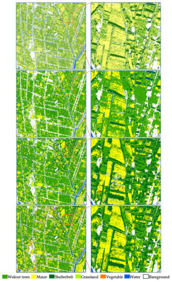
Figure 9.
Crop classification maps of F3 combinations: (A) MLC classification results; (a) Sample area of (A); (B) SVM classification results; (b) Sample area of (B); (C) RF classification results; (c) Sample area of (C); (D) RoF-SVM classification results; (d) Sample area of (D).
The classification accuracy of the MLC is 63.46%, that of the SVM is 80.15% and that of the RF is 84.11%. The corresponding kappa coefficients are valued at 0.61, 0.72, 0.76 respectively. However, the accuracy of RoF-SVM is 86.87%, and the kappa coefficient is 0.78. Compared with the three classification methods, the proposed RoF-SVM achieved a significantly higher level of classification accuracy. In the classification results of the four methods, the map derived via MLC showed evident “salt and pepper phenomena”. Many walnut trees are classified as maize and are visibly reduced relative to actual walnut plantations. The confusion of maize, vegetables, and grassland is considerable. This may mainly be attributed to the high-density intercropping area considered, and the selected GF-2 remote image acquisition period is the crop growth period, which is very similar in textural and spectral features. However, the MLC must assume that the spectral features of training samples are normally distributed, which is less realistic in the case of discrete and complex samples. Relative to the MLC results, the SVM classification reduces “salt and pepper phenomenon” and improves the OA by 16.69%. The producer and user accuracy levels of all types of vegetation cover show distinct improvements. The RF classification result is further improved relative to those of the SVM, and its OA reaches a value of 84.11%, which is very close to that of the RoF-SVM.
The RoF-SVM significantly increases user and producer accuracy levels for nearly all categories. The water body is continuously distributed and presents pronounced spectral features. Each classification result is highly accurate. However, in the MLC classification, some dried-out canals along the road are divided into water bodies. Serious interference is observed in the intercropping area. The accuracy of the classification of walnut trees and crops with the RoF-SVM was markedly improved. Errors in the shelterbelt are mainly observed in irregular and mixed walnut fields, and because populus bolleana usually reach heights of 1.2 m~20 m, some small trees were shaded by large trees. The shadow of the shelterbelt also leads to errors in the results for bare ground, grass, and crops.
5. Conclusions
Intercropping proves to offer many advantages and is a common cropping pattern. Remote sensing monitoring is important in estimating potential yields and tree–crop system management patterns. However, few remote sensing studies have addressed the issue of intercropping. This study developed a comprehensive feature extraction and intercropping classification scheme. Chinese GF-1 and GF-2 images were selected to explore the efficiency of vegetation classification for the intercropping area by using an ensemble classifier and rotation forest using the SVM as a base classifier (RoF-SVM). Walnut and maize intercropping areas in Moyu County south of the Tarim Basin were selected as the study area. To evaluate optimal feature selection, three group feature combinations derived from GF-1 and GF-2 images were combined, and the RoF-SVM ensemble learning method was adopted to classify the three groups. The group that combined spectral-textural-multitemporal features achieved the best classification results. Then, the classification results were compared with those of the MLC and SVM via optimal feature selection.
Therefore, GF-1 and GF-2 satellite images combined with spectral, textural, and multi-temporal features can provide sufficient information on vegetation cover in intercropping areas. At the same time, because such images are less expensive than other high-resolution images of the same resolution, they may be the preferred data source for crop monitoring and ecological environment assessments.
In the area of intercropping trees and crops, multi-feature and multi-temporal information can improve the differentiation of various objects and increase the classification accuracy. With the addition of textural features derived from a GLCM, the recognition of textures is greatly enhanced, and the distinction of trees and crops is greatly improved. Combining phenological information on the classified objects and selecting vegetation indices of specific temporal imagery can improve the classification accuracy of different types of trees and crops.
The proposed RoF-SVM offers the advantages of ensemble learning methods, offers the advantages of base classifiers (SVM algorithm) and enhances the level of diversity between individual base classifiers from a rotation forest. Therefore, different types of trees and crops in intercropping areas can be effectively distinguished (the OA was measured at 86.87 and the kappa coefficient was measured at 0.78). Moreover, classification results effectively eliminated salt and pepper noise.
Author Contributions
All of the authors made significant contributions to the work. Ping Liu contributed to the experiments, analyzed the results and wrote the paper. Xi Chen helped edit and review the manuscript.
Funding
This study was supported through the Strategic Priority Research Program of Chinese Academy of Sciences (Grant No. XDA20060303) and the International Cooperation Fund of Ecological Effects of Climate Change and Land Use/Cover Change in Arid and Semiarid Regions of Central Asia in the Most Recent 500 Years (Grant No. 41361140361).
Acknowledgements
The author is grateful to the editors and reviewers for their valuable comments and suggestions, from which the paper was revised.
Conflicts of Interest
The authors declare no conflicts of interest.
References
- Food and Agriculture Organization of the United Nations. Available online: http://www.fao.org/forestry/agroforestry/en/ (accessed on 1 August 2018).
- Smith, J.; Pearce, B.D.; Wolfe, M.S. Reconciling productivity with protection of the environment: Is temperate agroforestry the answer? Renew. Agric. Food Syst. 2013, 28, 80–92. [Google Scholar] [CrossRef]
- Wolz, K.J.; DeLucia, E.H. Alley cropping: Global patterns of species composition and function. Agric. Ecosyst. Environ. 2018, 252, 61–68. [Google Scholar] [CrossRef]
- Suroshe, S.S.; Chorey, A.B.; Thakur, M.R. Productivity and economics of maize-based intercropping systems in relation to nutrient management. Res. Crop. 2009, 10, 38–41. [Google Scholar]
- Waldner, F.; Canto, G.S.; Defourny, P. Automated annual cropland mapping using knowledge-based temporal features. ISPRS J. Photogramm. Remote Sens. 2015, 110, 1–13. [Google Scholar] [CrossRef]
- Begue, A.; Arvor, D.; Bellon, B.; Betbeder, J.; de Abelleyra, D.; Ferraz, R.P.D.; Lebourgeois, V.; Lelong, C.; Simoes, M.; Veron, S.R. Remote Sensing and Cropping Practices: A Review. Remote Sens. 2018, 10, 99. [Google Scholar] [CrossRef]
- Pringle, M.J.; Schmidt, M.; Tindall, D.R. Multi-decade, multi-sensor time-series modelling-based on geostatistical concepts-to predict broad groups of crops. Remote Sens. Environ. 2018, 216, 183–200. [Google Scholar] [CrossRef]
- Waldner, F.; Lambert, M.-J.; Li, W.; Weiss, M.; Demarez, V.; Morin, D.; Marais-Sicre, C.; Hagolle, O.; Baret, F.; Defourny, P. Land Cover and Crop Type Classification along the Season Based on Biophysical Variables Retrieved from Multi-Sensor High-Resolution Time Series. Remote Sens. 2015, 7, 10400–10424. [Google Scholar] [CrossRef]
- Belgiu, M.; Csillik, O. Sentinel-2 cropland mapping using pixel-based and object-based time-weighted dynamic time warping analysis. Remote Sens. Environ. 2018, 204, 509–523. [Google Scholar] [CrossRef]
- Hartfield, K.A.; van Leeuwen, W.J.D. Woody Cover Estimates in Oklahoma and Texas Using a Multi-Sensor Calibration and Validation Approach. Remote Sens. 2018, 10, 632. [Google Scholar] [CrossRef]
- Culvenor, D.S. TIDA: An algorithm for the delineation of tree crowns in high spatial resolution remotely sensed imagery. Comput. Geosci. 2002, 28, 33–44. [Google Scholar] [CrossRef]
- Mayossa, P.K.; D’Eeckenbrugge, C.; Borne, F.; Gadal, S.; Viennois, G. Developing a method to map coconut agrosystems from high-resolution satellite images. Proceedings of International Cartographic Conference, Rio de Janeiro, Brazil, 23–25 August 2015. [Google Scholar]
- China Centre for Resources Satellite Data and Application. Available online: http://www.cresda.com/EN/ (accessed on 1 December 2017).
- Chinese GF Application Integrated Information Service Sharing Platform. Available online: http://gfplatform.cnsa.gov.cn/ (accessed on 10 October 2017).
- Zhou, Q.-B.; Yu, Q.-Y.; Liu, J.; Wu, W.-B.; Tang, H.-J. Perspective of Chinese GF-1 high-resolution satellite data in agricultural remote sensing monitoring. J. Integr. Agric. 2017, 16, 242–251. [Google Scholar] [CrossRef]
- Jia, K.; Liang, S.; Gu, X.; Baret, F.; Wei, X.; Wang, X.; Yao, Y.; Yang, L.; Li, Y. Fractional vegetation cover estimation algorithm for Chinese GF-1 wide field view data. Remote Sens. Environ. 2016, 177, 184–191. [Google Scholar] [CrossRef]
- Arun, P.V.; Buddhiraju, K.M.; Porwal, A. CNN based sub-pixel mapping for hyperspectral images. Neurocomputing 2018, 311, 51–64. [Google Scholar] [CrossRef]
- Sonobe, R.; Yamaya, Y.; Tani, H.; Wang, X.; Kobayashi, N.; Mochizuki, K.-I. Crop classification from Sentinel-2-derived vegetation indices using ensemble learning. J. Appl. Remote Sens. 2018, 12. [Google Scholar] [CrossRef]
- Rodriguez-Galiano, V.F.; Chica-Olmo, M.; Abarca-Hernandez, F.; Atkinson, P.M.; Jeganathan, C. Random Forest classification of Mediterranean land cover using multi-seasonal imagery and multi-seasonal texture. Remote Sens. Environ. 2012, 121, 93–107. [Google Scholar] [CrossRef]
- Rodriguez, J.J.; Kuncheva, L.I. Rotation forest: A new classifier ensemble method. IEEE Trans. Pattern Anal. Mach. Intell. 2006, 28, 1619–1630. [Google Scholar] [CrossRef] [PubMed]
- Du, P.; Samat, A.; Waske, B.; Liu, S.; Li, Z. Random Forest and Rotation Forest for fully polarized SAR image classification using polarimetric and spatial features. ISPRS J. Photogramm. Remote Sens. 2015, 105, 38–53. [Google Scholar] [CrossRef]
- Lv, F.; Han, M. Hyperspectral Image Classification Based on Improved Rotation Forest Algorithm. Sensors 2018, 18, 3601. [Google Scholar] [CrossRef]
- Kussul, N.; Lavreniuk, M.; Skakun, S.; Shelestov, A. Deep Learning Classification of Land Cover and Crop Types Using Remote Sensing Data. IEEE Geosci. Remote Sens. Lett. 2017, 14, 778–782. [Google Scholar] [CrossRef]
- Huang, X.; Hu, T.; Li, J.Y.; Wang, Q.; Benediktsson, J.A. Mapping Urban Areas in China Using Multisource Data With a Novel Ensemble SVM Method. IEEE Trans. Geosci. Remote Sens. 2018, 56, 4258–4273. [Google Scholar] [CrossRef]
- Krawczyk, B.; Minku, L.L.; Gama, J.; Stefanowski, J.; Wozniak, M. Ensemble learning for data stream analysis: A survey. Inf. Fusion 2017, 37, 132–156. [Google Scholar] [CrossRef]
- Lin, L.; Zuo, R.; Yang, S.; Zhang, Z. SVM ensemble for anomaly detection based on rotation forest. Proceedings of Third International Conference on Intelligent Control and Information Processing, Dalian, China, 15–17 July 2012; pp. 150–153. [Google Scholar]
- Statistics Bureau of Xinjiang Uygur Autonomous Region. Available online: http://www.xjtj.gov.cn/sjcx/tjnj_3415/2016xjtjnj/ny/201707/t20170714_539607.html (accessed on 11 January 2019).
- Wang, J.; Wusiman, A.; Yusupu, A.; Aiqiong, W.U.; Xia, J.; Zhang, D.J. Analysis about Wheat Growth and Yield Formation in Walnut/Wheat Intercropping System. Acta Agriculturae Boreali-occidentalis Sinica. 2016, 25, 1289–1296. [Google Scholar]
- Wang, Q.; Blackburn, G.A.; Onojeghuo, A.O.; Dash, J.; Zhou, L.; Zhang, Y.; Atkinson, P.M. Fusion of Landsat 8 OLI and Sentinel-2 MSI Data. IEEE Trans. Geosci. Remote Sens. 2017, 55, 3885–3899. [Google Scholar] [CrossRef]
- Yokoya, N.; Grohnfeldt, C.; Chanussot, J. Hyperspectral and Multispectral Data Fusion A comparative review of the recent literature. IEEE Geosci. Remote Sens. Mag. 2017, 5, 29–56. [Google Scholar] [CrossRef]
- Liu, J.; Huang, J.Y.; Liu, S.G.; Li, H.L.; Zhou, Q.M.; Liu, J.C. Human visual system consistent quality assessment for remote sensing image fusion. ISPRS J. Photogramm. Remote Sens. 2015, 105, 79–90. [Google Scholar] [CrossRef]
- Shao, Z.F.; Cai, J.J. Remote Sensing Image Fusion With Deep Convolutional Neural Network. IEEE J. Sel. Top. Appl. Earth Observ. Remote Sens. 2018, 11, 1656–1669. [Google Scholar] [CrossRef]
- Zhou, X.; Liu, J.; Liu, S.; Cao, L.; Zhou, Q.; Huang, H. A GIHS-based spectral preservation fusion method for remote sensing images using edge restored spectral modulation. ISPRS J. Photogramm. Remote Sens. 2014, 88, 16–27. [Google Scholar] [CrossRef]
- Gasparovic, M.; Jogun, T. The effect of fusing Sentinel-2 bands on land-cover classification. Int. J. Remote Sens. 2018, 39, 822–841. [Google Scholar] [CrossRef]
- Gašparović, M.; Medak, D.; Pilaš, I.; Jurjević, L.; Balenović, I. Fusion of sentinel-2 and planetscope imagery for vegetation detection and monitoring. Int. Arch. Photogramm. Remote Sens. Spat. Inf. Sci. 2018, XLII-1, 155–160. [Google Scholar] [CrossRef]
- Maurer, T. How to pan-sharpen images using the Gram-Schmidt pan-sharpen method—A recipe. Int. Arch. Photogramm. Remote Sens. Spat. Inf. Sci. 2013, XL-1/W1, 239–244. [Google Scholar] [CrossRef]
- Roy, D.P.; Kovalskyy, V.; Zhang, H.K.; Vermote, E.F.; Yan, L.; Kumar, S.S.; Egorov, A. Characterization of Landsat-7 to Landsat-8 reflective wavelength and normalized difference vegetation index continuity. Remote Sens. Environ. 2016, 185, 57–70. [Google Scholar] [CrossRef]
- Huett, C.; Koppe, W.; Miao, Y.; Bareth, G. Best Accuracy Land Use/Land Cover (LULC) Classification to Derive Crop Types Using Multitemporal, Multisensor, and Multi-Polarization SAR Satellite Images. Remote Sens. 2016, 8, 684. [Google Scholar] [CrossRef]
- Baret, F.; Clevers, J.; Steven, M.D. The Robustness of Canopy Gap Fraction Estimates From Red And Near-Infrared Reflectances—A Comparison Of Approaches. Remote Sens. Environ. 1995, 54, 141–151. [Google Scholar] [CrossRef]
- Jiang, Z.; Huete, A.R.; Didan, K.; Miura, T. Development of a two-band enhanced vegetation index without a blue band. Remote Sens. Environ. 2008, 112, 3833–3845. [Google Scholar] [CrossRef]
- Bolton, D.K.; Friedl, M.A. Forecasting crop yield using remotely sensed vegetation indices and crop phenology metrics. Agric. For. Meteorol. 2013, 173, 74–84. [Google Scholar] [CrossRef]
- Huete, A.; Didan, K.; Miura, T.; Rodriguez, E.P.; Gao, X.; Ferreira, L.G. Overview of the radiometric and biophysical performance of the MODIS vegetation indices. Remote Sens. Environ. 2002, 83, 195–213. [Google Scholar] [CrossRef]
- Huang, X.; Liu, X.B.; Zhang, L.P. A Multichannel Gray Level Co-Occurrence Matrix for Multi/Hyperspectral Image Texture Representation. Remote Sens. 2014, 6, 8424–8445. [Google Scholar] [CrossRef]
- Wang, T.; Zhang, H.S.; Lin, H.; Fang, C.Y. Textural-Spectral Feature-Based Species Classification of Mangroves in Mai Po Nature Reserve from Worldview-3 Imagery. Remote Sens. 2016, 8, 15. [Google Scholar] [CrossRef]
- Lan, Z.Y.; Liu, Y. Study on Multi-Scale Window Determination for GLCM Texture Description in High-Resolution Remote Sensing Image Geo-Analysis Supported by GIS and Domain Knowledge. ISPRS Int. Geo-Inf. 2018, 7, 24. [Google Scholar] [CrossRef]
- Xiu, Y.; Liu, W.; Yang, W. An Improved Rotation Forest for Multi-Feature Remote-Sensing Imagery Classification. Remote Sens. 2017, 9, 1205. [Google Scholar] [CrossRef]
- Belgiu, M.; Dragut, L. Random forest in remote sensing: A review of applications and future directions. ISPRS J. Photogramm. Remote Sens. 2016, 114, 24–31. [Google Scholar] [CrossRef]
- Georganos, S.; Grippa, T.; Vanhuysse, S.; Lennert, M.; Shimoni, M.; Kalogirou, S.; Wolff, E. Less is more: Optimizing classification performance through feature selection in a very-high-resolution remote sensing object-based urban application. GISci. Remote Sens. 2018, 55, 221–242. [Google Scholar] [CrossRef]


© 2019 by the authors. Licensee MDPI, Basel, Switzerland. This article is an open access article distributed under the terms and conditions of the Creative Commons Attribution (CC BY) license (http://creativecommons.org/licenses/by/4.0/).