Abstract
Extracting the latent knowledge from Twitter by applying spatial clustering on geotagged tweets provides the ability to discover events and their locations. DBSCAN (density-based spatial clustering of applications with noise), which has been widely used to retrieve events from geotagged tweets, cannot efficiently detect clusters when there is significant spatial heterogeneity in the dataset, as it is the case for Twitter data where the distribution of users, as well as the intensity of publishing tweets, varies over the study areas. This study proposes VDCT (Varied Density-based spatial Clustering for Twitter data) algorithm that extracts clusters from geotagged tweets by considering spatial heterogeneity. The algorithm employs exponential spline interpolation to determine different search radiuses for cluster detection. Moreover, in addition to spatial proximity, textual similarities among tweets are also taken into account by the algorithm. In order to examine the efficiency of the algorithm, geotagged tweets collected during a hurricane in the United States were used for event detection. The output clusters of VDCT have been compared to those of DBSCAN. Visual and quantitative comparison of the results proved the feasibility of the proposed method.
1. Introduction
The dramatic increase in the popularity of social networks has resulted in the production of enormous amounts of “user-generated” data on a daily basis. Twitter, as one of the most popular and fast-growing microblogging services [1], produces over 500 million tweets per day (http://www.internetlivestats.com/twitter-statistics/) On the other hand, the advent of smart devices equipped with Global Navigation Systems has made it possible to share location in addition to the content of tweets. Daily generation of geotagged tweets has enabled scientists to look for advanced techniques to explore the latent knowledge and spatial patterns in various contexts including rumor diffusion [2], user activity pattern mining [3], crime type modeling [4], determining the relationship between social media attitudes and health outcomes [5], and extracting the users’ communities and discussed topics [6], to name but a few. Among other things, users of Twitter share messages and report information about events they have witnessed (e.g., flooding, earthquakes, hurricanes, tsunamis, terrorist attacks, accidents, festivals, etc.). Monitoring and analysis of such stream of user-generated data can provide invaluable information about events which would have never been possible to gather from traditional methods and resources [7,8]. Having the dynamic information about events, extracted from tweets, enables decision-makers to comprehend what is happening on the field and react appropriately.
Clustering, as a common technique for statistical data analysis [9,10], is an efficient method for event extraction from Twitter data [8]. The main idea of applying clustering algorithms on Twitter data is to decompose the dataset into similar groups of tweets that represent events. Using spatial clustering techniques, the entire dataset can be divided into several homogeneous subsets [11]. In other words, tweets which are related to each other in close locations have to be grouped together in the same clusters.
However, geotagged tweets are affected by spatial heterogeneity. The non-stationarity of the underlying spatial processes that result in an uneven distribution of a phenomenon in the study area is known as spatial heterogeneity [12]. In some areas, due to the population density or the combination of people living in the neighborhood, the number of active Twitter users and consequently the number of shared tweets is by far higher than other areas. For example, in areas with higher population density, we expect to receive more tweets than the areas with lower population density. Additionally, the age, level of education and economic condition result in a lower or higher number of shared tweets in various areas [13]. E.g., students prefer to use the internet and social media more than other groups and retired people are least likely to be internet users. Even the race of people affects the number of active users (http://www.pewinternet.org/2014/02/25/) of Twitter [14,15,16]. Therefore, the distribution of shared tweets is not similar in different locations and hence, heterogeneous over the study area. Utilizing appropriate clustering methods which consider spatial heterogeneity in geotagged tweets provides the effective means to detect the events from Twitter datasets. Moreover, the contents of the tweets are noisy, they usually include informal languages, smileys and location spoofing. We also do not have prior knowledge about the topic they discussed. Hence, in order to extract events, we need a clustering method that can simultaneously consider spatial proximities and textual similarities, is capable of extracting clusters with arbitrary shapes in noisy environments, and also requires the minimum number of input parameters.
Among existing clustering approaches, density-based algorithms, particularly DBSCAN (density-based spatial clustering of applications with noise) and its variations, are more efficient for detecting clusters with arbitrary shapes from noisy datasets where there is no prior knowledge about the number of clusters [17,18]. Due to its advantages, DBSCAN has been used in several studies to detect clusters and extract events from Twitter data [19,20,21]. C.-H. Lee [22] developed an online density-based algorithm for online spatio-temporal event detection from Twitter data. Arcaini et al. [23] proposed a method that first filters the tweets based on the users’ queries and then an extended DBSCAN algorithm, named GT-DBSCAN, is employed to explore the latent spatio-temporal pattern of tweets and extract events. Capdevila et al. [19] proposed Tweet-SCAN, as an extension to DBSCAN, which considers four main features of a tweet including content, time, location and user for tweet clustering. Nakahori and Yamaguchi [21] developed a tour minder system based on DBSCAN algorithm to mine tour plans in Twitter data. DBSTexC was also developed to extract spatio-textual cluster from Twitter data [24]. Although the mentioned studies utilized or extended DBSCAN algorithm to efficiently extract events from geotagged tweets, they did not consider the spatial heterogeneity in the twitter datasets.
Despite its wide application, DBSCAN is not efficient when there is spatial heterogeneity in the data and the density of the phenomenon significantly fluctuates over the study area [25,26,27]. In order to address this deficiency, Liu, Zhou, and Wu [26] proposed VDBSCAN (varied density-based spatial clustering of applications with noise) algorithm to account for spatial heterogeneity in the data by considering different parameters for cluster detection in each area based on the density in that area. However, the method which is utilized in VDBSCAN to determine local parameters is not appropriate for a large volume of data as it is the case for event detection from geotagged tweets.
This study proposes an algorithm called VDCT (Varied Density-based spatial Clustering for Twitter data), as an extension to VDBSCAN, to detect and extract geo-located events from Twitter data in existence of spatial heterogeneity. In addition to handling noise, extracting clusters of arbitrary shapes and requiring no prior knowledge about the number of clusters, VDCT is able to find clusters of geotagged tweets with varied densities. The algorithm considers both spatial proximity of geotagged tweets along with their text similarities. The algorithm is efficient to work with large volume of Twitter data. In order to evaluate the efficiency of the algorithm, a case-study related to event detection from geotagged tweets collected during a hurricane in the United States was considered. The outputs of VDCT were quantitatively and visually compared with those of DBSCAN.
2. Materials and Methods
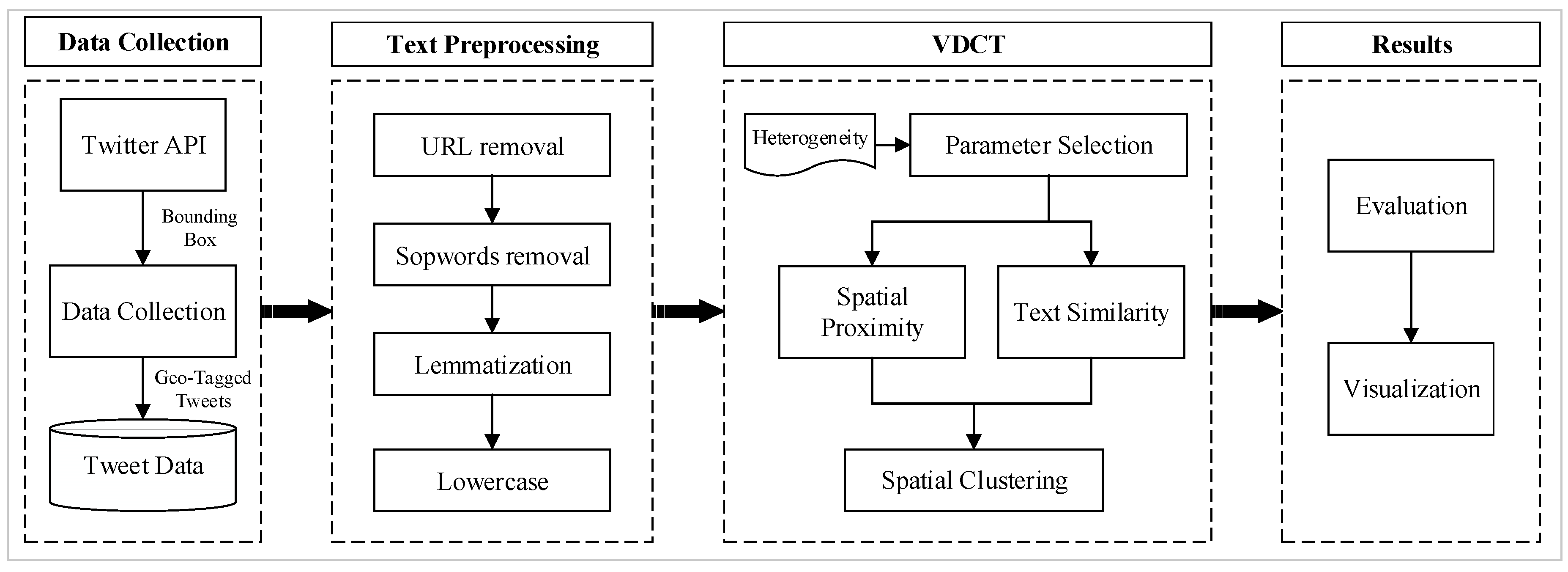
The overall workflow of the proposed approach for event detection from geotagged tweets is illustrated in Figure 1. The process starts with data collection using Twitter Streaming API where geotagged tweets (tweets that include latitude and longitude) are collected and saved. In order to prepare tweets for spatial clustering, text preprocessing is performed to transform tweets’ contents into words which can be used in the following processes. In the clustering step, the proposed clustering algorithm is used to extract spatial clusters from geo-located tweets. Finally, the outputs are evaluated and visualized.
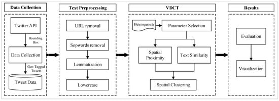
Figure 1.
Processing workflow.
2.1. Case-Study and Data Collection
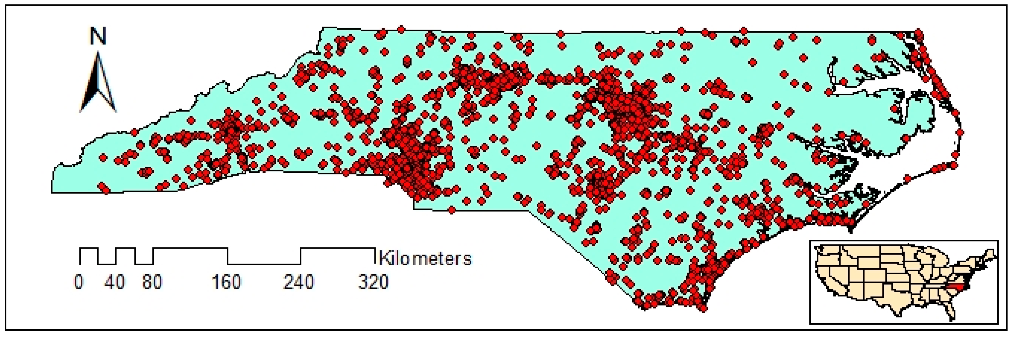
Hurricane Florence is selected as the case study to test how the proposed method can detect spatial events from geotagged tweets. As a Category 1 hurricane, Florence was predicted to have maximum wind speeds between 74 and 95 kph. Powerful waves and walls of water moved inland and led to flooding. North Carolina State was severely affected by the hurricane and was selected as the study area in this research. Using Twitter streaming API, shared tweets within North Carolina have been collected during hurricane Florence, from 12 September to 19 September. Tweets were filtered using bounding box and only tweets which contain latitude and longitude were extracted and saved in the database.
2.2. Text Processing
In order to use the extracted tweets for spatial clustering, a text preprocessing phase is required. Initially, URLs, hashtags, special characters, and numbers are removed. Then, the words are converted to lowercase and stop words are deleted. Finally, the rest of the words are transformed into their stem form through lemmatization. After the text preprocessing, 8992 geotagged tweets remained in the study area. The final extracted tweets are presented in Figure 2.
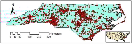
Figure 2.
Distribution of geotagged tweets.
2.3. VDCT
In order to cluster geo-located tweets and extract events, a varied density-based clustering algorithm, named VDCT (Varied Density-based spatial Clustering for Twitter data), was developed in this study. Consider T as a collection of geotagged tweets so that each tweet is represented as a tuple , where and are the geographical coordinate of the tweet, is the textual content of the tweet and is the cluster label of the tweet which is undefined at the beginning. VDCT algorithm receives as input and return , so that every tweet in the result set, , has a defined cluster label, , or its cluster label is set to noise, .
2.3.1. Text Similarity
In order to extract events, similar tweets must be placed in the same clusters. In this regard, in addition to Euclidean distance between geotagged tweets, the text similarity of tweets should be considered. Text similarity plays an important role in document clustering and topic modeling [28,29]. As tweets are limited to 140 characters, most of the text similarity techniques are not efficient for calculating the similarity between them due to the short length of the messages, the informal language and a large number of spelling and grammatical errors [30,31]. Meanwhile, cosine similarity is a similarity measure which has proved its ability to calculate the text similarity between tweets [32,33]. Cosine similarity in text mining is a string-based measure which measures the distance between two strings. Each string represented by a vector. Consider W as the collection of all terms in T. For a tweet , its textual content can be presented as vector , where shows the number of times the term occurs in tweet . Having two tweets and , their similarity is computed according to cosine formula (Equation (1)) [3].
Cosine similarity measures the cosine of the angle between two non-zero vectors. If two vectors are perpendicular, they have cosine similarity of 0 and when they are similar and completely the same, they have cosine similarity of 1.
2.3.2. Clustering
The proposed VDCT solution for extracting clusters from geotagged Twitter data is an extension to the DBSCAN algorithm. DBSCAN receives two parameters of epsilon and minimum points (minPnts) as inputs, where epsilon is the radius for neighborhood search and minPnts is the minimum number of points that must exist around a data point so that those points can be considered as a cluster. DBSCAN randomly selects a point which at least has minPnts points within the distance of epsilon around it. The surrounding points are called reachable points afterward. The selected point and its reachable points are considered as a cluster. The cluster will repeatedly grow by adding other points that are in the epsilon distance of the reachable points as new reachable points. The algorithm continues until all points are either has a cluster label or there is less than minPnts points around them and thus they are considered as noise [17].
In order to address the shortcoming of DBSCAN in dealing with spatial heterogeneity, VDBSCAN (varied density-based spatial clustering of applications with noise) algorithm was proposed by Liu, Zhou, and Wu [26]. VDBSCAN chooses different values for epsilon using k-dist plot. For all data points in the dataset, the average distances to the k neighbors of each point are computed, sorted in ascending order and plotted in a graph where x-axis shows the distance (epsilon) and y-axis depicts the points sorted by the distance. The sharp changes in the plot correspond to the suitable epsilon values. In this method, when the density varies significantly in different regions, various values of epsilon are determined [26].
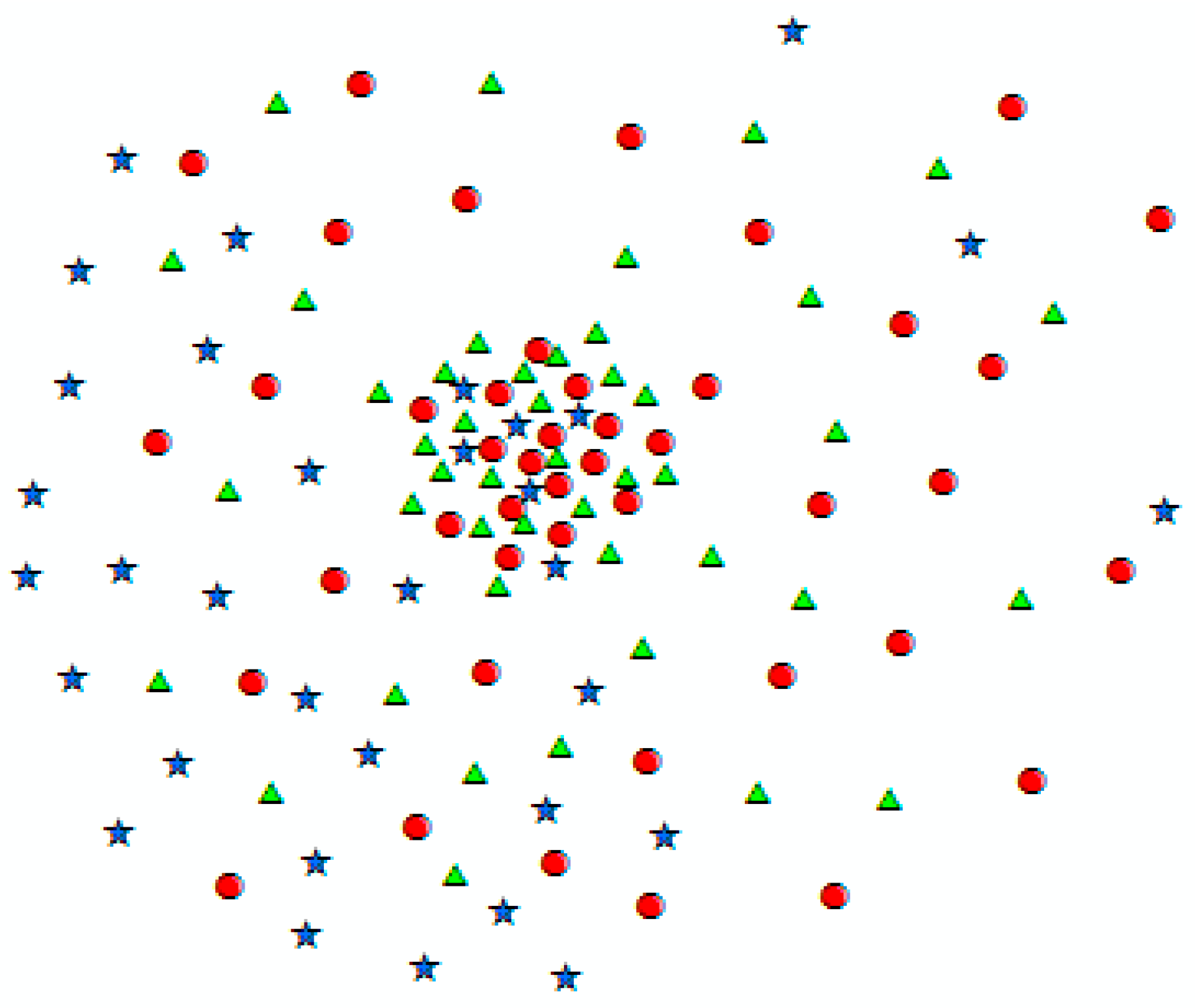
Although VDBSCAN can effectively deal with spatial heterogeneity, it still encounters two main challenges for event extraction from Twitter data. The first challenge is that VDBSCAN only considers one dimension for cluster detection. However, in order to develop an effective event detection algorithm for Twitter data, the algorithm must consider the similarity between the content of tweets in addition to closeness in space. As illustrated in Figure 3, tweets at the center of the image are geographically close, but they refer to different contents and therefore cannot be grouped in the same cluster. The second challenge is that VDBSCAN, in order to deal with spatial heterogeneity, utilizes k-dist plot to determine the epsilon parameter for various densities. However, k-dist plot is efficient for small data and does not perform well when we are dealing with large datasets [34] such as Twitter data. Particularly, it is hard to detect the sharp changes in the plot when there exists a large number of data points.

Figure 3.
Tweets with various contents.
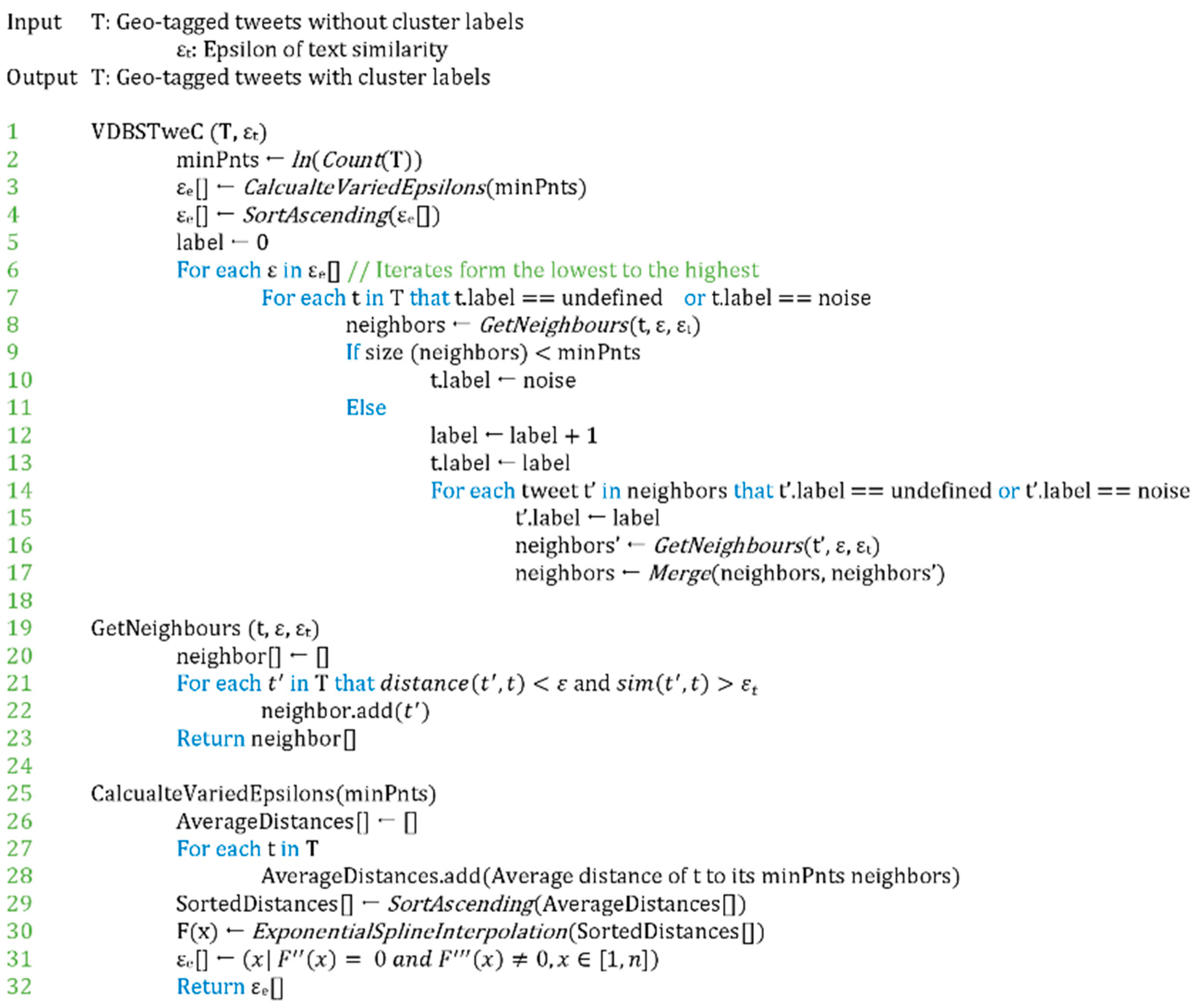
In order to address the mentioned shortcomings, VDCT considers both location and text similarity for cluster detection by including two neighborhood search parameters of and for spatial proximity and text similarity, respectively. Additionally, the proposed algorithm borrows the idea of calculating various values for neighborhood search from VDBSCAN, but uses exponential spline interpolation, instead of k-dist plot to find the different levels of densities. Figure 4 represents the pseudo code of VDCT algorithm.
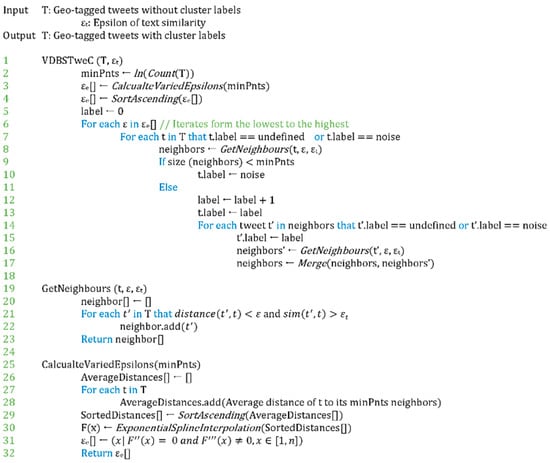
Figure 4.
The pseudo code of VDCT algorithm.
As it is described in Figure 4, the algorithm receives geotagged tweets (T) and text similarity search radius () as input. Each tweet in T contains both geographical coordinates and textual content, but the cluster labels of the tweets are undefined. The algorithm starts by calculating minPnts (Figure 4, line 3), which is the minimum number of tweets that must exist in the neighborhood of a tweet so that those tweets can be considered as a cluster. A heuristic approach for choosing a proper minPnts is through calculating ln(n), where n is the total number of input tweets [35,36].
In order to calculate (Figure 4, line 3 and lines 22 to 29), as the varied radiuses for neighborhood search, k-nearest neighbor distances are calculated using kd-tree data structure. Employing kd-tree leads the computation of k-nearest neighbors (k-NN) to be more efficient which is crucial for handling large datasets [37,38]. The value of k is set to minPnts value [39]. The average distances to k nearest neighbors are calculated afterwards and sorted in an ascending order. Based on the recommendation of Louhichi, Gzara, and Ben-Abdallah [34], exponential splines interpolation [40] is used then to extract different levels of densities. In this approach, an exponential spline curve is fitted to the sorted average distances of k nearest neighbors. Having the exponential spline curve, inflection points, the points at which the direction of curvature changes, are extracted and considered as the candidates of different density levels and therefore values. Bronshtein et al. [41] has thoroughly described the procedure of extracting inflection points from exponential splines.
After calculating the values of , they are sorted in ascending order. Then, by iterating through the lowest value to the highest value of εe, the algorithm tries to find clusters with different densities and assign cluster labels to tweets while considering both εe and (Figure 4, lines 6 to 17). In each iteration, a tweet that hasn’t given a cluster label before (a tweet with the label of undefined or noise) is selected and its neighbors are listed. If the number of selected neighbors is less than minPnts, then the tweet is considered as a noise. Otherwise, the tweet and its neighbors are considered as a new cluster; they receive a new label; and the algorithm tries to expand this cluster and find other tweets around these tweets that are included in this cluster (Figure 4, lines 16 and 17) by searching for the neighbors of the tweets in the neighbor list and merging the results into the neighbor list. The expansion continuous until all the tweets in the current cluster are found and labeled. Then, the algorithm continues with the next value of .
In order to the select the neighbor of a tweet (Figure 4, lines 19 to 23), both Euclidean distance between tweets and text similarity are considered. Two tweets are considered as neighbors if the Euclidean distance between them is less than and their text similarity, calculated based on cosine formula (Equation (1)), is greater than εt.
2.4. Quality Measures
Selection of proper measures for the evaluation of clustering algorithms depends on the available information and utilized methods [42,43]. Two types of evaluation measures have been used in the literature: internal indices and external indices. While external indices compare the results with the existing ground truth, internal measures compare the results of different algorithms to show which algorithm performs better. Using internal evaluation criteria, the output clusters with high intra-similarity and low inter-similarity get higher scores. Due to the fact that it is very hard to collect ground truth data for events that are already happening in the real world, three internal measures of Davies–Bouldin index [44], Dunn index [45] and Silhouette coefficient [46] have been used in this study to compare the results of the proposed clustering algorithms with the results of DBSCAN as the base algorithm. Davies–Bouldin index is calculated using Equation (2).
In Equation (2), n is the number of clusters, is the centroid of cluster x, is the average distance of all objects of cluster x to the centroid of cluster and d(ci, ci) depicts the distance between centroids of clusters i and j. According to this criteria, the algorithm which produces the lowest Davies–Bouldin index is considered to perform better.
Dunn index calculates the ratio between the minimum inter-cluster distances to the maximum intra-cluster distance [45]. This index is calculated using Equation (3).
In Equation (3), is the inter-cluster distance between clusters i and j and is the distance between objects in cluster k. The distance between clusters i and j can be calculated using various methods such as measuring the distance between centroids of the clusters. The algorithm which achieves higher Dunn index is more efficient.
The silhouette coefficient contrasts the average distance to objects in the same cluster with the average distance to the objects in other clusters [46]. The coefficient ranges between −1 and 1 where 1 represents the best value. Negative values show that samples are wrongly assigned to a cluster. Overlapping clusters result in values near 0. The following equation calculates the silhouette coefficient.
In Equation (4), is the distance between an object and the nearest cluster that the object does not belong to and a(i) is the mean intra-cluster distance of an object.
3. Results and Discussion
In addition to geotagged tweets, is the only input parameter of the proposed algorithm. The algorithm received 8992 geotagged tweets, related to Hurricane Florence (Section 2.1), while the value of was set to 0.5. The algorithm was able to assign cluster labels to the input tweets. In order to provide a reference for comparison, we also ran a DBSCAN algorithm on the dataset with minPnts = 10 and epsilon = 0.1.
3.1. Parameter Sselection
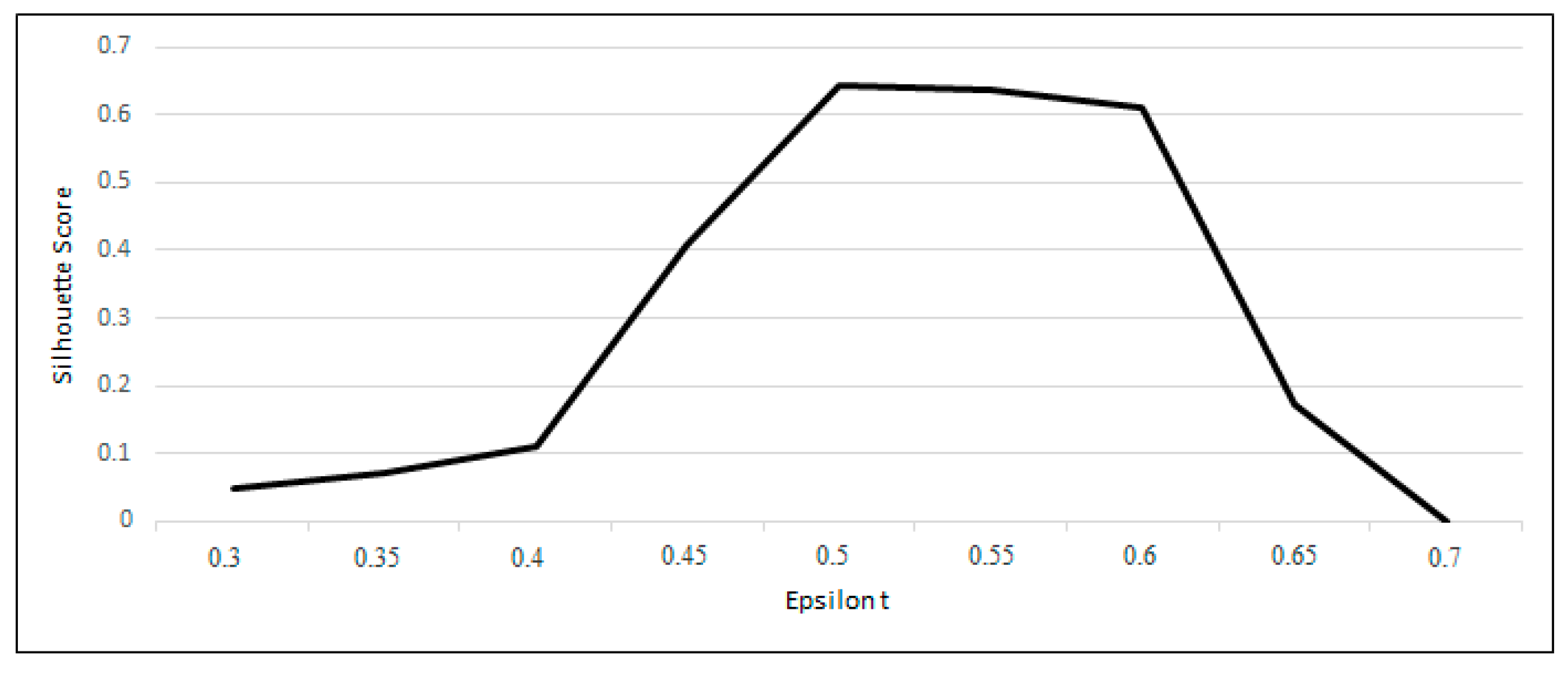
In order to obtain the best value of εt that maximizes the performance of the proposed solution, the model was run with different values of , from 0.3 to 1, and the silhouette scores was calculated for the output results. As it can be seen in Figure 5, the value of 0.5 for results in the highest silhouette score. For the εt value of 0.7, VDCT only extracted one cluster and hence the silhouette score was equal to zero. For the values higher than 0.7, no cluster was detected, and no silhouette score was calculated. Therefore, the value of 0.5 has been chosen for text similarity threshold which is also in line with the best text similarity threshold that was used in the literature [47,48,49,50].
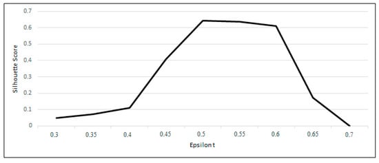
Figure 5.
Variation of the silhouette coefficient in response to different values.
3.2. Quality Measures’ Results
The output results of VDCT and DBSCAN algorithms are presented in Table 1. According to the results, the value of Dunn index and silhouette coefficient of VDCT are higher than those of DBSCAN. Also, VDCT achieved lower Davies–Bouldin index than DBSCAN. The output results prove that VDCT provides more satisfactory results in comparison with DBSCAN.

Table 1.
The output results of internal evaluation criteria.
3.3. Visual Comparison and Discussion
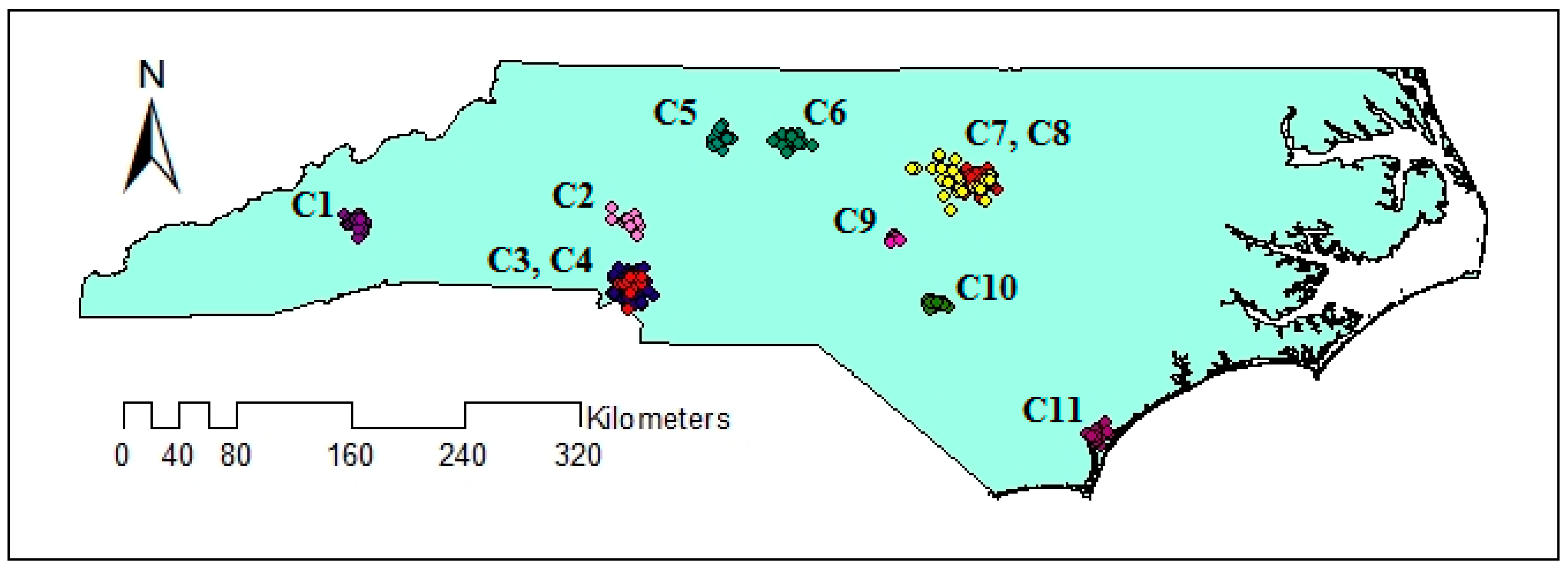
The distribution of geotagged tweets from 12 September to 19 September is illustrated in Figure 2. The figure shows that the distribution of geotagged tweets varies over the study area and therefore, there may be clusters with varied densities. The extracted clusters using VDCT and DBSCAN clustering algorithms are demonstrated in Figure 6 and Figure 7, respectively, where 11 clusters have been extracted by VDCT and 8 clusters have been determined by DBSCAN. The location of the extracted clusters by both algorithms are almost the same. However, VDCT extracted clusters with more details and higher accuracy in comparison with DBSCAN. In addition, the sizes of clusters detected by VDCT are different from those of DBSCAN.
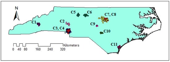
Figure 6.
Extracted clusters using VDCT clustering algorithm.

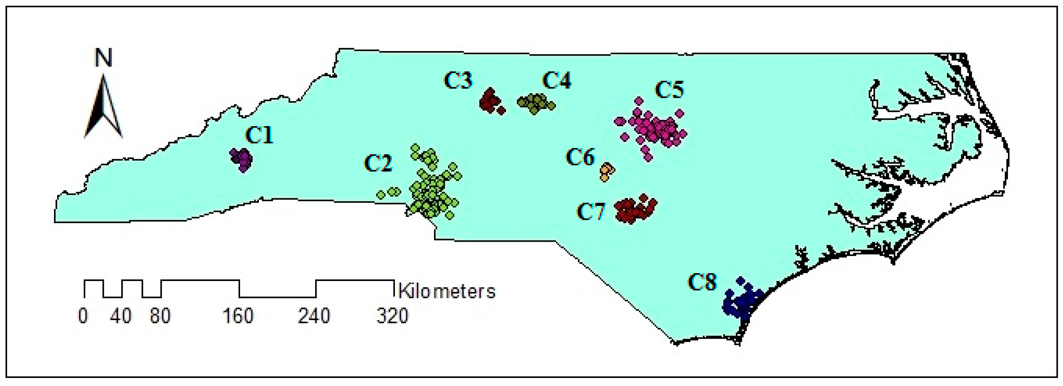
Figure 7.
Extracted clusters using DBSCAN clustering algorithm.
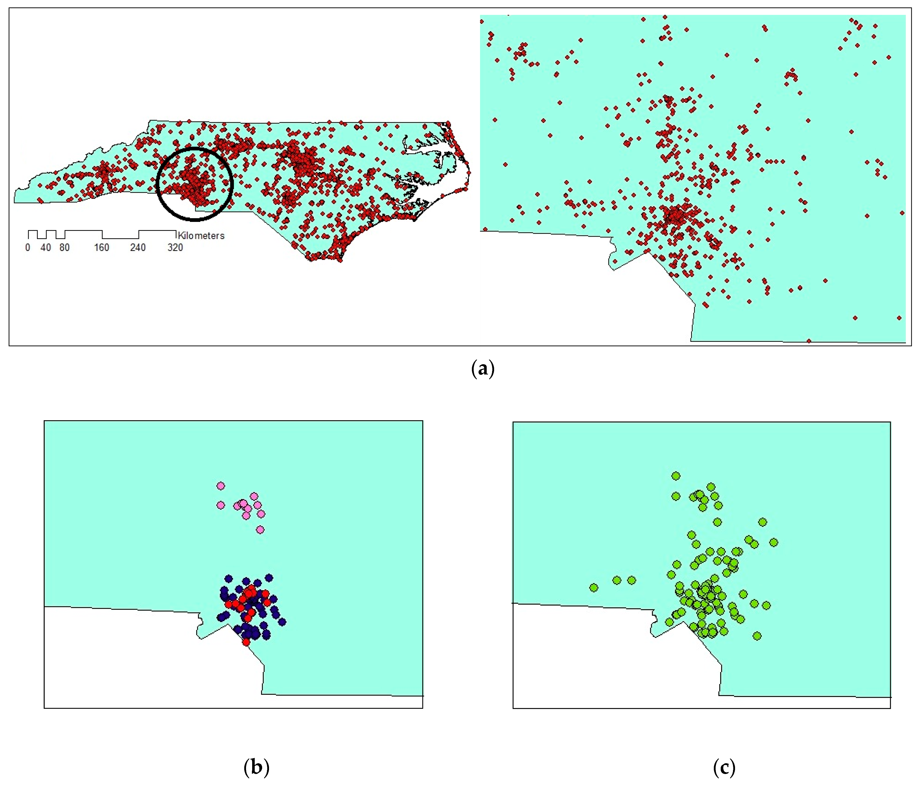
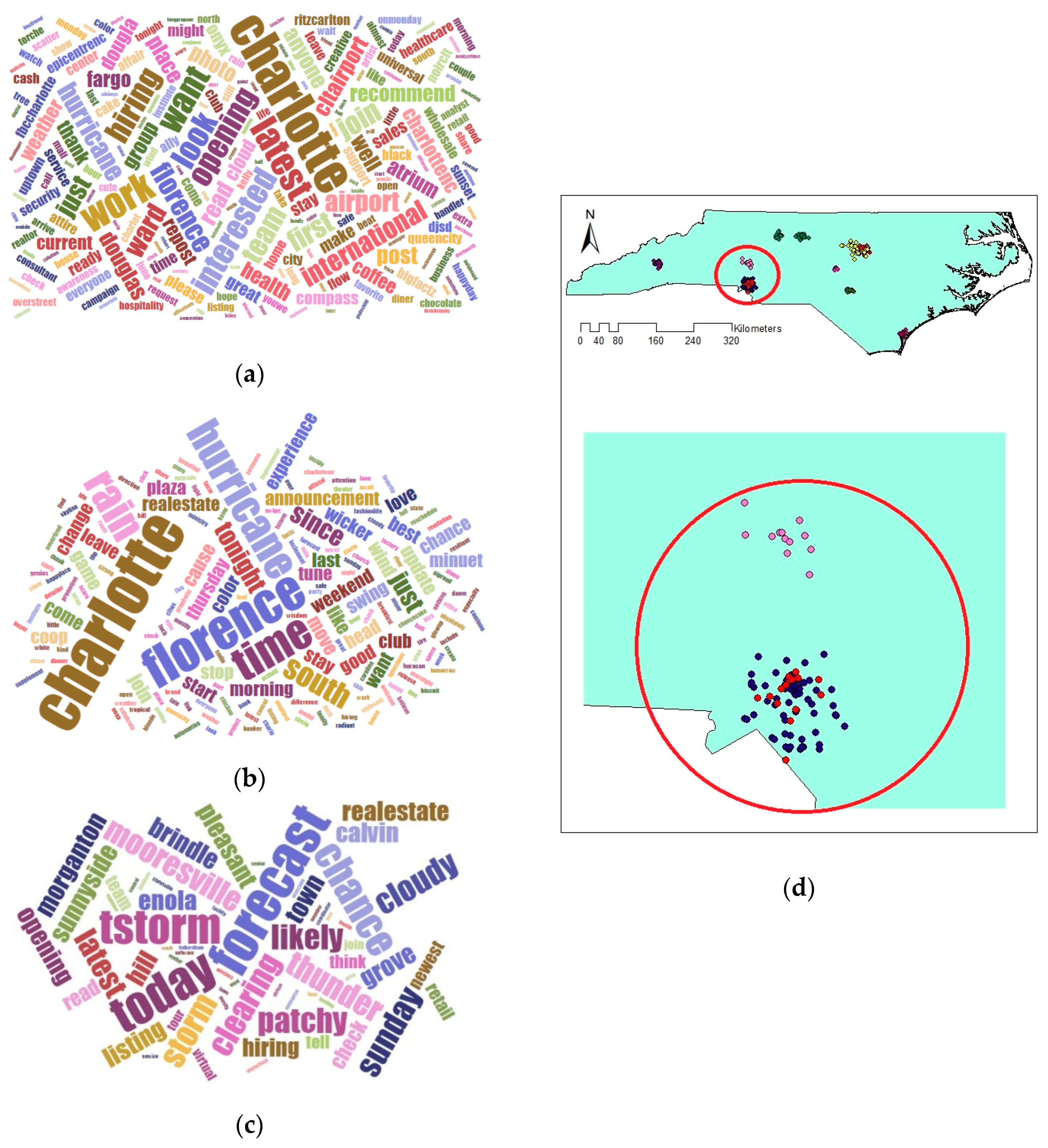
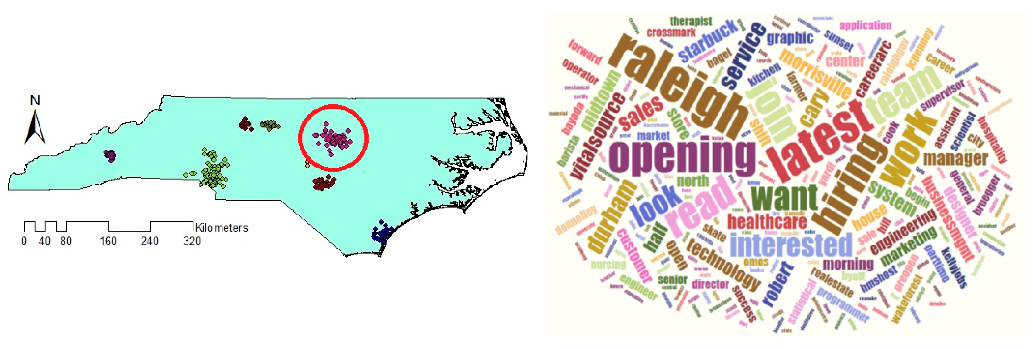
Comparing the size and content of the extracted clusters by the algorithms clarifies that in the areas with less density variation, VDCT and DBSCAN extracted clusters which are almost the same. While in the areas with higher variation in densities, the algorithms perform differently. In these areas, VDCT extracted more clusters with different densities. A part of the study area with higher variation in density is depicted in Figure 8. As it is shown in Figure 8a, by considering different values for , VDCT was able to extract 3 distinct clusters (C2, C3 and C4, Figure 6) while DBSCAN clustered all data of this area into only one group (C2, Figure 7). The Word Cloud of cluster C2 of DBSCAN and clusters C2, C3 and C4 of VDCT are illustrated in Figure 9 and Figure 10a–c, respectively. Word Cloud is a visualization method which displays the frequency and importance of each word in a document by its size. The Word Cloud of VDCT clusters indicates that the proposed algorithm was able to appropriately separate clusters related to the hurricane and other topics. The most frequent words are “forecast”, “tstorm” and “today” in cluster C4, “charlotte”, “Florence” and “hurricane” in cluster C3 and “charlotte”, “opening”, “work” and “hiring” in cluster C2. While all these tweets are clustered together by DBSCAN algorithm. The other clear distinctions between the output clusters are cluster C5 of DBSCAN and C7 and C8 of VDCT. As depicted in Figure 11 and Figure 12, two distinct clusters extracted by VDCT are grouped as a unique cluster by DBSCAN. VDCT separated clusters related to “Raleigh” event and its “Opening”. While DBSCAN clustered all tweets related to “Raleigh” to one group.

Figure 8.
(a) A part of the study area with more variation in density; (b) Extracted clusters by VDCT and (c) Extracted clusters by DBSCAN.
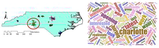
Figure 9.
Word Cloud generated for Cluster number 2 (C2) of DBSCAN.
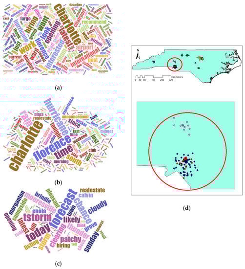
Figure 10.
Word Cloud generated for Clusters (a) 2, (b) 3 and (c) 4 extracted by VDCT and (d) their positions on map.

Figure 11.
Word Cloud generated for Cluster 5 of DBSCAN.
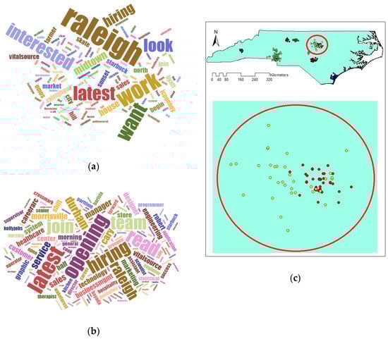
Figure 12.
Word Cloud generated for Clusters (a) 7 and (b) 8 extracted by VDCT and (c) their positions on map.
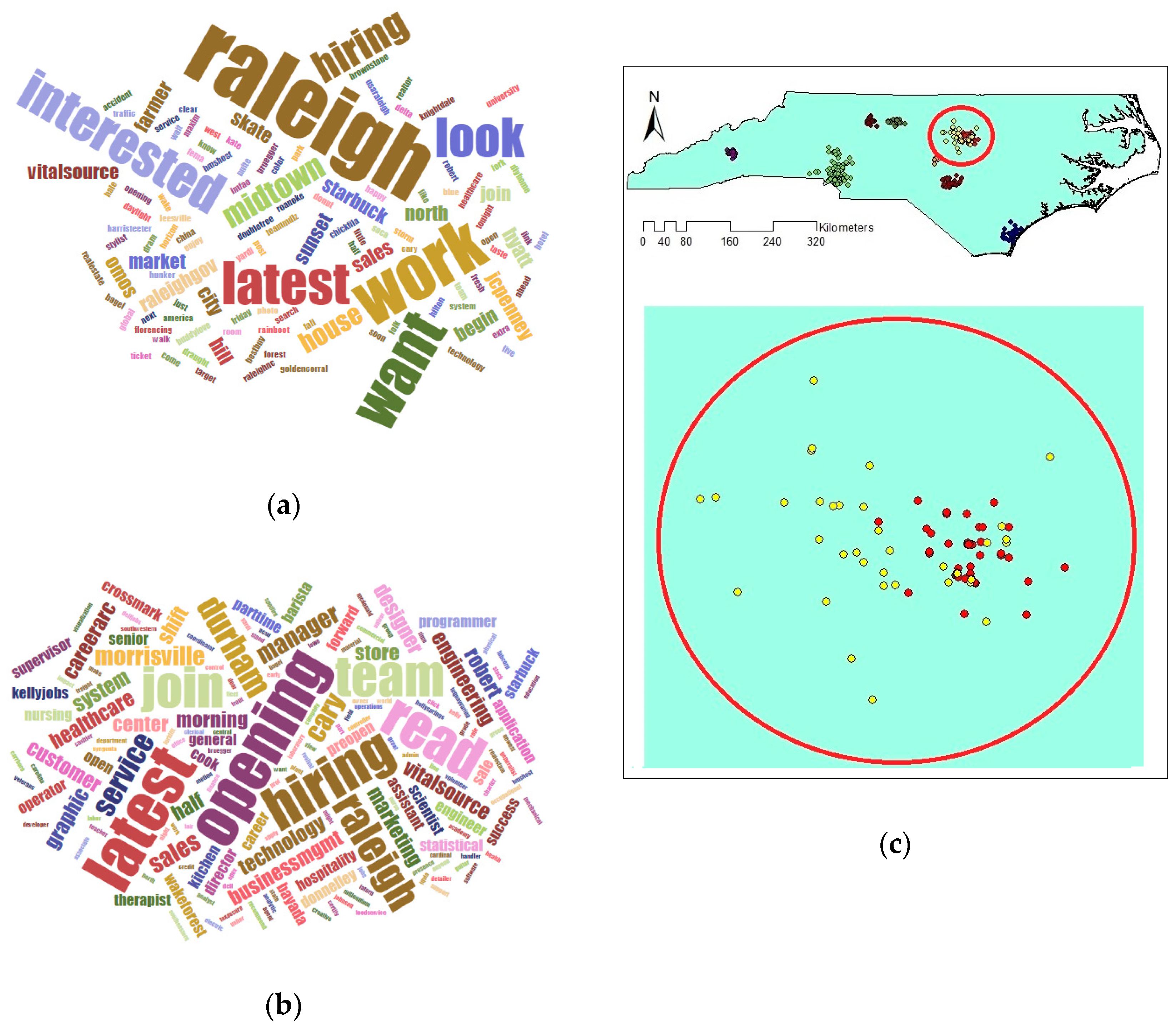
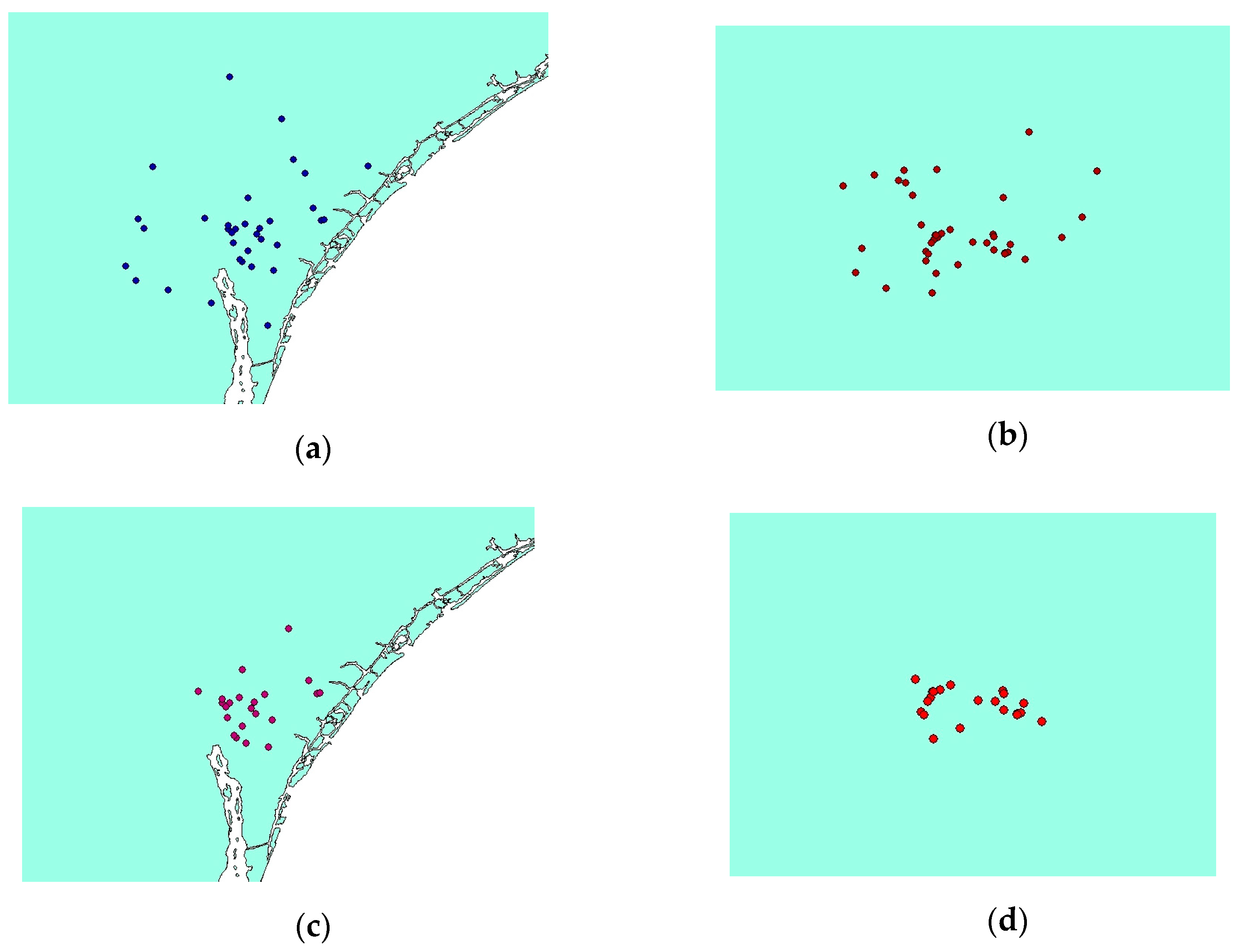
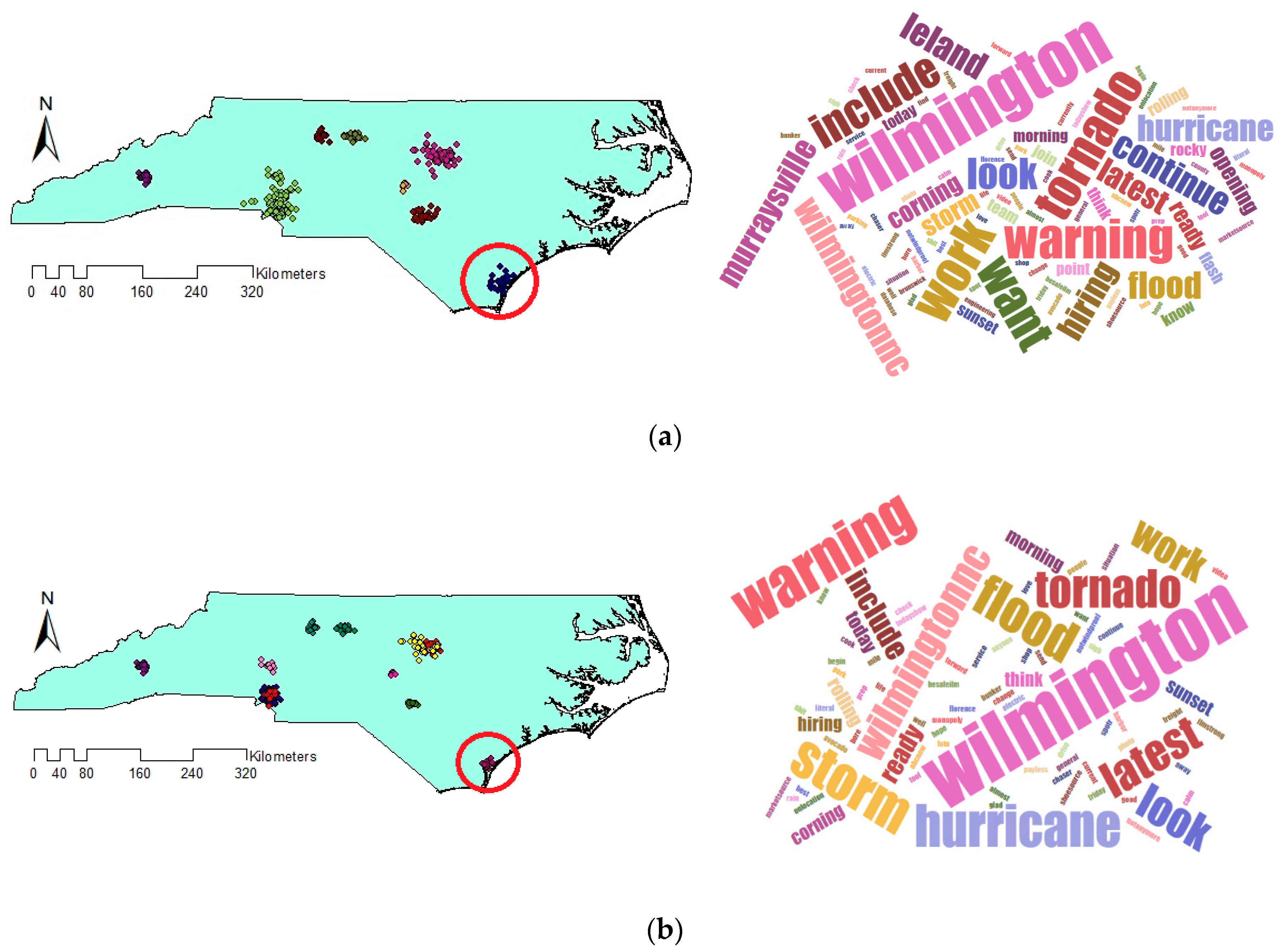
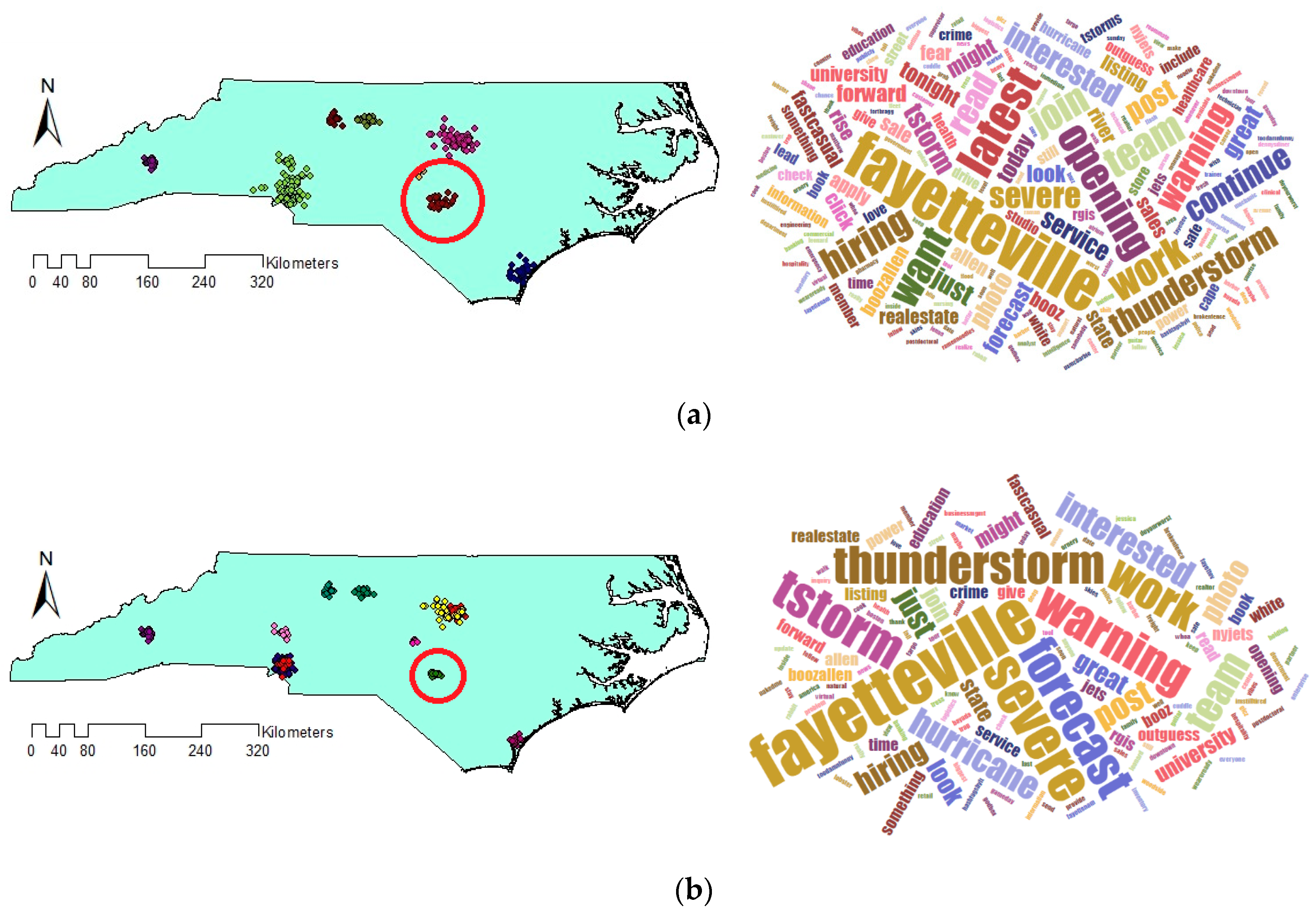
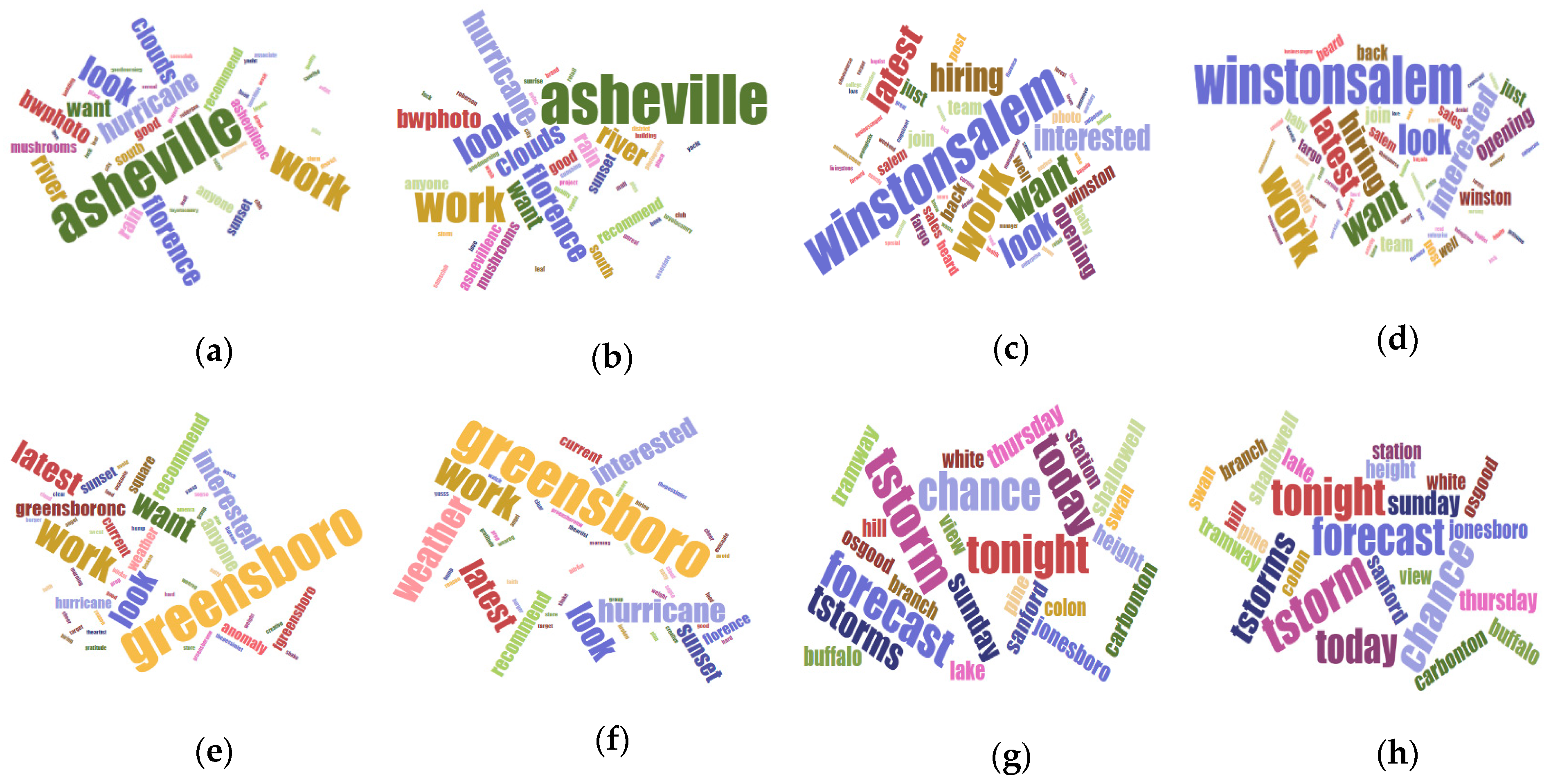
The other crucial issue that should be noticed is the different sizes of output clusters. Figure 13 demonstrates the extracted clusters of algorithms which are located at the same places but with diverse sizes. As clusters are located at the same location, they are indicating the same events. But the extracted clusters by VDCT are smaller than those of DBSCAN. Smaller and more compact clusters seem to be more useful since they provide us with the ability to monitor specific incidents rather than large clusters which may present both the event and the surrounding area. An example is Figure 11, in which VDCT separated tweets relating to “Raleigh” and its “opening” while DBSCAN considered all these tweets as one cluster. Another example is cluster C8 of DBSCAN and C11 of VDCT which their Word Clouds are illustrated in Figure 14a,b, respectively. The extracted Word Clouds and frequent words indicate that both clusters point to the same event which is “hurricane” in “Wilmington”. Having more tweets with irrelevant words to the hurricane, the frequency and importance of words related to hurricane such as “warning”, “flood”, “tornado” are affected by the existence of other words and therefore their sizes are diminished in the Word Cloud of the DBSCAN cluster. However, in VDCT extracted cluster, words such as “warning”, “hurricane”, “flood” and “storm” can be clearly distinguished. It is the same for clusters C7 of DBSCAN and C10 of VDCT which their Word Cloud are illustrated in Figure 15a,b, respectively. The frequent words, “thunderstorm”, “tstorm”, “severe”, “warning” and “forecast” can be quickly recognized in VDCT cluster, while these words cannot be easily identified in DBSCAN cluster as they are affected by other words. The other clusters (C1, C5, C6 and C9 of VDCT and C1, C3, C4 and C6 of DBSCAN) are almost the same for both algorithms as the density of tweets does not significantly vary in these places and their Word Clouds depict the same frequent words in related clusters. The generated Word Clouds of these clusters are illustrated in Figure 16.
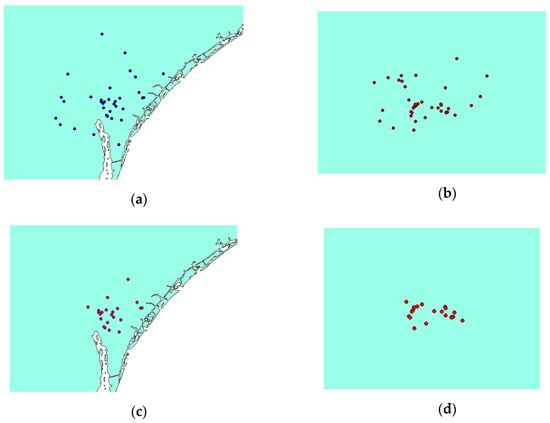
Figure 13.
Clusters (a) number 8 of DBSCAN, (b) number 7 of DBSCAN, (c) number 11 of VDCT and (d) number 10 of VDCT.
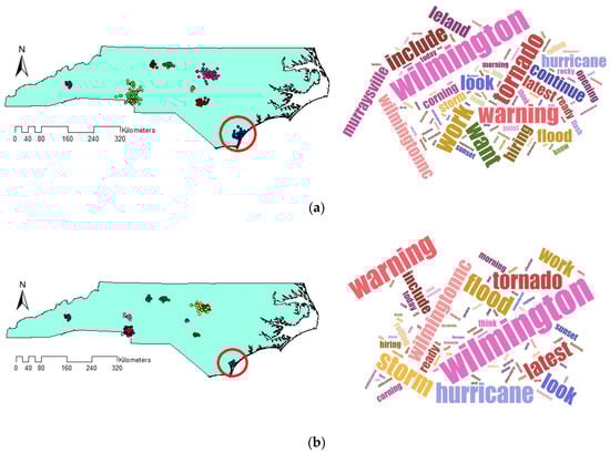
Figure 14.
Generated Word Cloud of (a) C8 DBSCAN and (b) C11 VDCT.
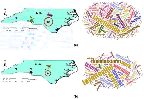
Figure 15.
Generated Word Cloud of (a) C7 DBSCAN and (b) C10 VDCT.
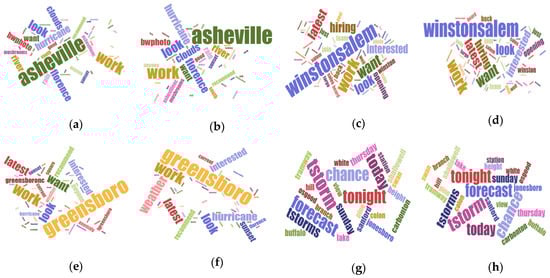
Figure 16.
Word Cloud generated for clusters: (a) C1, (c) C3, (e) C4 and (g) C6 of DBSCAN and (b) C1, (d) C5, (f) C6 and (h) C9 of VDCT.
An important issue about the presented Word Clouds of the clusters (Figure 8, Figure 9, Figure 10, Figure 11, Figure 12, Figure 13, Figure 14, Figure 15 and Figure 16) is the existence of the names of the places near the main event in the Word Clouds. Although these place names can be considered redundant words from one aspect, they still convey valuable information that can be helpful in determining the location of the events. If we consider an event which has happened in a special place, the users from other areas may share some tweets related to that event. These tweets may create a cluster. However, the words in the Word Cloud of the cluster do not match with its surrounding location names. By considering the name of the surrounding locations and the Word Cloud of the cluster, the events which happened in other places can be identified and single out. There are some studies in this regard that have tried to localize the extracted clusters based on the location names in each area [51,52,53,54].
4. Conclusions and Future Works
This study proposed a solution for event extraction from geotagged tweets. In order to overcome the shortcomings of DBSCAN in dealing with density variation in the Twitter dataset, VDBSCAN algorithm has been extended to extract clusters from geotagged tweets. The proposed algorithm, VDCT, employs exponential spline interpolation to determine different search radiuses for cluster detection. It also utilizes cosine similarity to group tweets with similar content in addition to spatial closeness. For evaluation, the output clusters of VDCT have been compared to those of DBSCAN. The results prove the ability of VDCT in extracting clusters with varied densities from geotagged tweets. In areas where density fluctuated, VDCT was able to extract more precise clusters with different densities and more details, while DBSCAN merged denser clusters into one in areas with significant variation in density. Also, the comparison of the content of the output clusters showed that VDCT was able to efficiently group tweets with more related contents, while DBSCAN clusters sometimes included some tweets with less similarity in context.
As depicted in output maps, the number of geotagged tweets considerably varies over different areas. Some areas consist of a considerable number of users who share a large number of tweets during weekdays while the others have only a few active users. So, in order to form a cluster, the number of minimum points can be set differently for different areas due to the number of active users in each area. In this regard, the future work will focus on determining different values for the minimum number of points for VDCT algorithm based on the number of active users in each area. Additionally, improving the proposed solution so that it can localize the extracted events by considering the names of the surrounding locations will be a field of future investigation. The other issue is that cosine similarity does not consider the semantics of the words. Utilizing semantic similarity measures to improve the result of spatial clustering is also considered as a future work of this study.
Author Contributions
Z.G. and M.F. conceived and designed the study and related experiments; both authors implemented the experiments and statistical analysis. Z.G. prepared the original draft. M.F. was the supervisor and reviewed and edited the manuscript. The manuscript was discussed and analyzed by both authors.
Funding
This research received no external funding.
Conflicts of Interest
The authors declare no conflict of interest.
References
- Adedoyin-Olowe, M.; Gaber, M.M.; Dancausa, C.M.; Stahl, F.; Gomes, J.B. A rule dynamics approach to event detection in twitter with its application to sports and politics. Expert Syst. Appl. 2016, 55, 351–360. [Google Scholar] [CrossRef]
- Serrano, E.; Iglesias, C.A.; Garijo, M. A survey of Twitter rumor spreading simulations. In Computational Collective Intelligence; Springer: Berlin/Heidelberg, Germany, 2015; pp. 113–122. [Google Scholar]
- Fu, C.; McKenzie, G.; Frias-Martinez, V.; Stewart, K. Identifying spatiotemporal urban activities through linguistic signatures. Comput. Environ. Urban Syst. 2018, 72, 25–37. [Google Scholar] [CrossRef]
- Gerber, M.S. Predicting crime using Twitter and kernel density estimation. Decis. Support Syst. 2014, 61, 115–125. [Google Scholar] [CrossRef]
- Relia, K.; Akbari, M.; Duncan, D.; Chunara, R. Socio-spatial Self-organizing Maps: Using Social Media to Assess Relevant Geographies for Exposure to Social Processes. arXiv 2018, arXiv:1803.09002. [Google Scholar] [CrossRef]
- Akbari, M.; Relia, K.; Elghafari, A.; Chunara, R. From the User to the Medium: Neural Profiling Across Web Communities. In Proceedings of the Twelfth International AAAI Conference on Web and Social Media, Palo Alto, CA, USA, 25–28 June 2018. [Google Scholar]
- Atefeh, F.; Khreich, W. A survey of techniques for event detection in twitter. Comput. Intell. 2015, 31, 132–164. [Google Scholar] [CrossRef]
- Arın, İ.; Erpam, M.K.; Saygın, Y. I-TWEC: Interactive clustering tool for Twitter. Expert Syst. Appl. 2018, 96, 1–13. [Google Scholar] [CrossRef]
- Mohammadinia, A.; Alimohammadi, A.; Saeidian, B. Efficiency of Geographically Weighted Regression in Modeling Human Leptospirosis Based on Environmental Factors in Gilan Province, Iran. Geosciences 2017, 7, 136. [Google Scholar] [CrossRef]
- Saeidian, B.; Mesgari, M.; Pradhan, B.; Ghodousi, M. Optimized Location-Allocation of Earthquake Relief Centers Using PSO and ACO, Complemented by GIS, Clustering, and TOPSIS. ISPRS Int. J. Geo-Inf. 2018, 7, 292. [Google Scholar] [CrossRef]
- Yang, W.; Deng, M.; Xu, F.; Wang, H. Prediction of hourly PM2. 5 using a space-time support vector regression model. Atmos. Environ. 2018, 181, 12–19. [Google Scholar] [CrossRef]
- Brunsdon, C.; Fotheringham, S.; Charlton, M. Geographically weighted regression. J. R. Stat. Soc. Ser. D (Stat.) 1998, 47, 431–443. [Google Scholar] [CrossRef]
- Blank, G. The digital divide among Twitter users and its implications for social research. Soc. Sci. Comput. Rev. 2017, 35, 679–697. [Google Scholar] [CrossRef]
- Sloan, L.; Morgan, J.; Burnap, P.; Williams, M. Who tweets? Deriving the demographic characteristics of age, occupation and social class from Twitter user meta-data. PLoS ONE 2015, 10, e0115545. [Google Scholar] [CrossRef] [PubMed]
- Sloan, L.; Morgan, J.; Housley, W.; Williams, M.; Edwards, A.; Burnap, P.; Rana, O. Knowing the tweeters: Deriving sociologically relevant demographics from Twitter. Sociol. Res. Online 2013, 18, 1–11. [Google Scholar] [CrossRef]
- Mislove, A.; Lehmann, S.; Ahn, Y.-Y.; Onnela, J.-P.; Rosenquist, J.N. Understanding the Demographics of Twitter Users. ICWSM 2011, 11, 25. [Google Scholar]
- Ester, M.; Kriegel, H.-P.; Sander, J.; Xu, X. A density-based algorithm for discovering clusters in large spatial databases with noise. In Proceedings of the KDD 1996, Portland, OR, USA, 2–4 August 1996; pp. 226–231. [Google Scholar]
- Parimala, M.; Lopez, D.; Senthilkumar, N. A survey on density based clustering algorithms for mining large spatial databases. Int. J. Adv. Sci. Technol. 2011, 31, 59–66. [Google Scholar]
- Capdevila, J.; Cerquides, J.; Nin, J.; Torres, J. Tweet-scan: An event discovery technique for geo-located tweets. Pattern Recognit. Lett. 2017, 93, 58–68. [Google Scholar] [CrossRef]
- Capdevila, J.; Pericacho, G.; Torres, J.; Cerquides, J. Scaling dbscan-like algorithms for event detection systems in twitter. In Proceedings of the International Conference on Algorithms and Architectures for Parallel Processing, Granada, Spain, 14–16 December 2016; pp. 356–373. [Google Scholar]
- Nakahori, K.; Yamaguchi, S. A method to discover spots from Twitter for tour miner. In Proceedings of the 2017 IEEE International Symposium on Consumer Electronics (ISCE), Taibei, Taiwan, 12–14 June 2017; pp. 32–34. [Google Scholar]
- Lee, C.-H. Mining spatio-temporal information on microblogging streams using a density-based online clustering method. Expert Syst. Appl. 2012, 39, 9623–9641. [Google Scholar] [CrossRef]
- Arcaini, P.; Bordogna, G.; Ienco, D.; Sterlacchini, S. User-driven geo-temporal density-based exploration of periodic and not periodic events reported in social networks. Inf. Sci. 2016, 340, 122–143. [Google Scholar] [CrossRef]
- Nguyen, M.D.; Shin, W.-Y. DBSTexC: Density-Based Spatio-Textual Clustering on Twitter. In Proceedings of Proceedings of the 2017 IEEE/ACM International Conference on Advances in Social Networks Analysis and Mining, Sydney, Australia, 31 July–3 August 2017; pp. 23–26. [Google Scholar]
- Idrissi, A.; Rehioui, H.; Laghrissi, A.; Retal, S. An improvement of DENCLUE algorithm for the data clustering. In Proceedings of the 2015 5th International Conference on Information & Communication Technology and Accessibility (ICTA), Marrakech, Morocco, 21–23 December 2015; pp. 1–6. [Google Scholar]
- Liu, P.; Zhou, D.; Wu, N. VDBSCAN: Varied density based spatial clustering of applications with noise. In Proceedings of the 2007 International Conference on Service Systems and Service Management, Chengdu, China, 8–11 June 2007; pp. 1–4. [Google Scholar]
- Ram, A.; Sharma, A.; Jalal, A.S.; Agrawal, A.; Singh, R. An enhanced density based spatial clustering of applications with noise. In Proceedings of the 2009 Advance Computing Conference, Patiala, India, 6–7 March 2009; pp. 1475–1478. [Google Scholar]
- Al-Smadi, M.; Jaradat, Z.; Al-Ayyoub, M.; Jararweh, Y. Paraphrase identification and semantic text similarity analysis in Arabic news tweets using lexical, syntactic, and semantic features. Inf. Process. Manag. 2017, 53, 640–652. [Google Scholar] [CrossRef]
- Lee, H.; Kihm, J.; Choo, J.; Stasko, J.; Park, H. iVisClustering: An interactive visual document clustering via topic modeling. Comput. Graph. Forum 2012, 1155–1164. [Google Scholar] [CrossRef]
- Hurlock, J.; Wilson, M.L. Searching Twitter: Separating the Tweet from the Chaff. In Proceedings of the Fifth International AAAI Conference on Weblogs and Social Media, Barcelona, Spain, 17–21 July 2011; pp. 161–168. [Google Scholar]
- Zuo, Y.; Wu, J.; Zhang, H.; Lin, H.; Wang, F.; Xu, K.; Xiong, H. Topic modeling of short texts: A pseudo-document view. In Proceedings of the 22nd ACM Sigkdd International Conference on Knowledge Discovery and Data Mining, San Francisco, CA, USA, 24–27 August 2016; pp. 2105–2114. [Google Scholar]
- Fu, C.; Samet, H.; Sankaranarayanan, J. WeiboStand: Capturing Chinese breaking news using Weibo tweets. In Proceedings of the 7th ACM Sigspatial International Workshop on Location-Based Social Networks, Dallas/Fort Worth, TX, USA, 4 November 2014; pp. 41–48. [Google Scholar]
- Sankaranarayanan, J.; Samet, H.; Teitler, B.E.; Lieberman, M.D.; Sperling, J. Twitterstand: News in tweets. In Proceedings of the 17th Acm sigspatial International Conference on Advances in Geographic Information Systems, Seattle, WA, USA, 4–6 November 2009; pp. 42–51. [Google Scholar]
- Louhichi, S.; Gzara, M.; Ben-Abdallah, H. Unsupervised varied density based clustering algorithm using spline. Pattern Recognit. Lett. 2017, 93, 48–57. [Google Scholar] [CrossRef]
- Suthar, N.; Jeet Rajput, I.; Kumar Gupta, V. A Technical Survey on DBSCAN Clustering Algorithm. Int. J. Sci. Eng. Res. 2013, 4, 1775–1781. [Google Scholar]
- Birant, D.; Kut, A. ST-DBSCAN: An algorithm for clustering spatial-temporal data. Data Knowl. Eng. 2007, 60, 208–221. [Google Scholar] [CrossRef]
- Bentley, J.L. Multidimensional binary search trees used for associative searching. Commun. ACM 1975, 18, 509–517. [Google Scholar] [CrossRef]
- Friedman, J.H.; Bentley, J.L.; Finkel, R.A. An algorithm for finding best matches in logarithmic expected time. ACM Trans. Math. Softw. 1977, 3, 209–226. [Google Scholar] [CrossRef]
- Garcia, J.C.; Avendaño, A.; Vaca, C. Where to go in Brooklyn: NYC Mobility Patterns from Taxi Rides. In Proceedings of the World Conference on Information Systems and Technologies, Naples, Italy, 27–29 March 2018; pp. 203–212. [Google Scholar]
- Schweikert, D.G. An interpolation curve using a spline in tension. J. Math. Phys. 1966, 45, 312–317. [Google Scholar] [CrossRef]
- Bronshtein, I.N.; Semendyayev, K.A.; Musiol, G.; Muehlig, H. Tables. In Handbook of Mathematics; Springer: Berlin/Heidelberg, Germany, 2004; pp. 1007–1091. [Google Scholar]
- Ghaemi, Z.; Alimohammadi, A.; Farnaghi, M. LaSVM-based big data learning system for dynamic prediction of air pollution in Tehran. Environ. Monit. Assess. 2018, 190, 300. [Google Scholar] [CrossRef]
- Saeidian, B.; Mesgari, M.S.; Ghodousi, M. Optimum allocation of water to the cultivation farms using Genetic Algorithm. Int. Arch. Photogramm. Remote Sens. Spat. Inf. Sci. 2015, 40, 31–38. [Google Scholar] [CrossRef]
- Davies, D.L.; Bouldin, D.W. A cluster separation measure. IEEE Trans. Pattern Anal. Mach. Intell. 1979, 224–227. [Google Scholar] [CrossRef]
- Dunn, J.C. Well-separated clusters and optimal fuzzy partitions. J. Cybern. 1974, 4, 95–104. [Google Scholar] [CrossRef]
- Rousseeuw, P.J. Silhouettes: A graphical aid to the interpretation and validation of cluster analysis. J. Comput. Appl. Math. 1987, 20, 53–65. [Google Scholar] [CrossRef]
- Chellal, A.; Boughanem, M.; Dousset, B. Word similarity based model for tweet stream prospective notification. In Proceedings of the European Conference on Information Retrieval, Aberdeen, UK, 8–13 April 2017; pp. 655–661. [Google Scholar]
- De Boom, C.; Van Canneyt, S.; Demeester, T.; Dhoedt, B. Representation learning for very short texts using weighted word embedding aggregation. Pattern Recognit. Lett. 2016, 80, 150–156. [Google Scholar] [CrossRef]
- Ozdikis, O.; Senkul, P.; Oguztuzun, H. Context based semantic relations in tweets. In State of the Art Applications of Social Network Analysis; Springer: Berlin/Heidelberg, Germany, 2014; pp. 35–52. [Google Scholar]
- Xu, W.; Callison-Burch, C.; Dolan, B. SemEval-2015 Task 1: Paraphrase and semantic similarity in Twitter (PIT). In Proceedings of the 9th International Workshop on Semantic Evaluation (SemEval 2015), Denver, CO, USA, 4–5 June 2015; pp. 1–11. [Google Scholar]
- Gelernter, J.; Balaji, S. An algorithm for local geoparsing of microtext. GeoInformatica 2013, 17, 635–667. [Google Scholar] [CrossRef]
- Xu, Z.; Chen, L.; Chen, G. Topic based context-aware travel recommendation method exploiting geotagged photos. Neurocomputing 2015, 155, 99–107. [Google Scholar] [CrossRef]
- Abdelhaq, H.; Sengstock, C.; Gertz, M. Eventweet: Online localized event detection from twitter. Proc. VLDB Endow. 2013, 6, 1326–1329. [Google Scholar] [CrossRef]
- Zhang, L.; Sun, X.; Zhuge, H. Location-driven geographical topic discovery. In Proceedings of the 2013 Ninth International Conference on Semantics, Knowledge and Grids (SKG), Beijing, China, 3–4 October 2013; pp. 210–213. [Google Scholar]

© 2019 by the authors. Licensee MDPI, Basel, Switzerland. This article is an open access article distributed under the terms and conditions of the Creative Commons Attribution (CC BY) license (http://creativecommons.org/licenses/by/4.0/).