Abstract
This paper presents an analysis of the effects of cognitive agents employing selfish routing behavior in traffic networks with linear latency functions. Selfish routing occurs when each agent traveling on a network acts in a purely selfish manner, therefore the Braess Paradox is likely to occur. The Braess Paradox describes a situation where an additional edge with positive capacity is added to a given network, which leads to higher total system delay. By applying the concept of cognitive agents, each agent is able to make a range of non-selfish and selfish decisions. In addition, each agent has to cope with uncertainty in terms of travel time information associated with the traffic system, a factor in real-world traffic networks. This paper evaluates the influence of travel time uncertainty, and possible non-selfish decisions of the agents on overall network delay. The results indicate that both non-selfish behavior and uncertainty have an influence on overall travel delay. In addition, understanding the influence of cognitive agents on delay can help to better plan and influence traffic flows resulting in “closer to optimal” flows involving overall lower delays.
1. Introduction
The shortest path problem is well studied in the literature and has been applied in many different types of applications in the field of Geographic Information Science and Technology that range from habitat connectivity to vehicle routing. Shortest path algorithms form the basis for personal and vehicle navigation, where a path of least travel time, travel cost, or some other metric is used. People tend to use navigation aids in order to find their way in unfamiliar environments. In addition, many cars are equipped with a built-in or mobile navigation system that is capable of receiving (near) real-time traffic information—e.g., closed roads or traffic congestion, and many may guide drivers to routes that are less congested (e.g., Waze). Many products like Waze give the same guidance to everyone, which can lead to creating new evolving areas of congestion.
Navigation is comprised of two activities “way finding” (planning) and “locomotion” (execution of movements) [1]. Due to the fact that (near) real-time information is now integrated into the navigation process, the separation between “planning” and “execution of movements”, described as wayfinding and locomotion in [1], appears to be diminishing. We argue that the separation of the processes wayfinding strictly happening before locomotion is questionable. In the literature, navigation is described in a way that the user selects a destination and one or a combination of costs (e.g., time, fuel cost, travel distance) that can be used in evaluating possible routes. Based on the chosen cost function the navigation system responds with the minimum cost route from the current location to the destination. This planning process is valid for non-dynamic traffic situations but does not consider traffic as a “living” system, that displays certain dynamics. This is due to the fact that there are a number of players on a road network, each making their own decisions, where those decisions affect in concert the state of the network in the future. Hence, the network and associated attributes are time-dependent, and an accurate deterministic prediction cannot be made. In order to find shortest paths in a dynamic network several methods have been developed [2,3,4,5,6]. These algorithms try to “react” to dynamic conditions in the road network, and identify one shortest path for exactly one agent navigating in the network in a given situation—i.e., network status within the time-frame of the shortest path traversal).
From the literature it is evident that route planning models are tailored towards one single user, and thus do not address the fact that other agents are also making their decisions, each impacting the outcomes of others. In order to simulate decisions of a group of agents, game theory is employed in the literature [7]. Braess [8] identified a problem in traffic modeling that has since been called “Braess Paradox”, which describes a situation where a given set of players in a traffic network each try to find their “best route” in a selfish manner. Hence, selfish players choose the fastest route from their own perspective, neglecting the effect for other players. Given that an extra edge is added to the network, a layman could assume that the average travel time of the players will be the same or lower than the original network layout as the overall capacity has been increased. For the Braess example, the travel times are higher than what happens on the original network without the extra edge.
Roughgarden [7] and Braess [8] both assume a non-cooperative game, where players are purely selfish. In this paper, we apply the concept of a group of cognitive agents where each agent/player is able to make decisions accordingly—and change the strategy accordingly. In order to investigate the effect of the behavior of cognitive agents the approach in this paper evaluates:
- Varying probabilities of agents acting in a non-selfish way.
- Varying levels of uncertainty in travel time information. That is, the information available on network congestion-status may be fuzzy for some agents.
The basic research question addressed in this paper is: “How do different compositions of selfish & non-selfish decisions of agents affect the delay or latency of all agents acting on the network, considering possible uncertainties in the information regarding network status?” The rationale behind the contributions of this paper is as follows. Due to the fact that selfish routing depends on selfish behavior of agents in a network, decisions can be considered to be crisp rather than fuzzy. This holds true for situations in which agents have accurate information on the network status and act purely selfish—one type of condition involving machines but probably never in a complete sense for humans. In a transport network with cognitive agents, we assume that each agent has the ability to act in a non-selfish way, as well as that traffic information may be defined as uncertain. The driver is not able to fully evaluate the accuracy of the traffic situation ahead, due to the following reasons:
- (a)
- Real-time traffic applications (like Waze) are dependent on the number of users collecting & providing data. Such real-time applications have a high market share in certain countries, but they do not have a significant market penetration in all regions of the earth. In some European capital cities the numbers of Waze users are at a maximum. For example, in Paris approximately 51,000 users per/1 million citizens use the app. Other cities lag behind, for example Vienna involves only 1000 users/1 million citizens [9].
- (b)
- Traffic Message Channels (TMC) provide traffic information for vehicle drivers sent via FM radio frequency. This information can be included into any satnav system for routing purposes. The system is designed so that traffic information is only provided for major traffic junctions/locations collected in a location table—which results in inaccuracies in the location and extent of any traffic congestion.
- (c)
- As TMC or FM radio provided traffic information requires that traffic information be collected, checked and published thereafter, there is a temporal delay between the incident and the publishing of the traffic information. In FM radio stations, the updates on traffic may be broadcasted every 30 min, which means an incident may have cleared by the time that the information is broadcasted.
- (d)
- As we deal with a dynamic situation, the traffic conditions ahead of an agent may alter as the agent moves toward an incident location that is along the desired route. Hence, any agent has to rely on a prediction on how the situation might change—especially when the agent does not receive any timely update on the situation as he/she comes closer to the incident location.
Therefore, the provided traffic information can be regarded as only partly accurate. An agent does not necessarily have full trust in the provided traffic information—as the situation might differ from what is expected when the agent arrives at the incident location. Generally speaking, in real world situations any agent in a network does not necessarily have an accurate, timely overview on the network status. Kattan et al. [10] concluded that commuters who sought information from many traffic update sources were likely to be more compliant with the traffic advice when they received it. Hence, agents do not necessarily react to traffic updates accordingly, when they only have one single source of information or when updates are less frequent.
A key component in Intelligent Transportation Systems (ITS) is to forecast the number of vehicles and their positions in a traffic system [11]. The traffic forecasting is done with the collection of current traffic data. These data are amended with ancillary data as well as a trip demand model. In literature a number of traffic forecast models have been proposed. The classic approach is the Four-Step model [12]. The theoretical approach of this model is based upon the decomposing the process into four steps: Trip generation, trip distribution, mode choice and route assignment. Route assignment describes the allocation of trips between origin and destination. Wardrop’s principle [13], equivalent to the Nash equilibrium, is applied in the route assignment step. This problem is a so-called bi-level problem, as the travel times are a function of the demand along route segments and demand is a function of travel time along those very same segments. Other approaches utilize the Stackelberg competition model, where agents in a traffic network respond to actions of a leading instance.
The contribution of the paper is as follows. With the help of agent-based approach we show that the behavior and the agents influence the overall latency. This aspect in itself is not new, but what is new is the fact that we model agents where they are provided traffic information where there is a degree of uncertainty as to its accuracy. Agent decisions based upon this uncertain information on the traffic status may decrease/increase the overall latency, as they tend to make “wrong” decisions with respect to the real network status and in relation to their chosen strategy (i.e., selfish verses non-selfish behavior).
This paper is organized as follows. In the next section the relevant literature is briefly discussed and analyzed, followed by a section on the methodology applied in this paper to evaluate the effect of cognitive agents displaying varying degrees of selfish routing behavior and reliance on imperfect traffic information. Section 4 presents the results and analysis, and is followed by a summary in the final section.
2. Network Flows, Routing Games and Selfish Routing
This section reviews the concepts of the maximum flow problem, the min-cost flow problem and relevant theory on routing games. Whereas forms of the minimum cost flow model can be used to solve for traffic flows that involve the lowest total network delay, selfish routing involves the concept where travelers on the network behave in a strictly selfish manner. Routing games are “games”, in the sense of game theory [14], that occur in non-cooperative situations, where several agents try to find the best strategy that increases their own benefit at a possible cost to others. Generally, agents alter their strategy to improve their own benefit until they cannot increase their benefit any further. This situation is described in literature as a state of equilibrium—or Nash equilibrium [15]. Overall, selfish routing is a result of different agents acting on a network, each trying to find the best path from a strictly personal viewpoint, regardless of the consequence for other agents.
2.1. Shortest Paths and Network Flows
To begin, let us define a basic set of terms that are used in this paper. A network, N = {V,E}, is a set of n nodes, V, and a set of m edges, E. Edges are assumed to be directed, i.e., each edge consists of an ordered pair of nodes. Roads segments that can be traversed in both directions are represented as two network edges, one for each direction of travel. Additionally, each edge is assigned a cost function that represents the travel time to traverse that edge, represented as ce:R+→R+. Such travel time functions are usually expressed as a function of traffic flow, and increases with increasing traffic. In most networks, a number of different directed paths exist that connect an origin or source node with a destination or node.
Network flow problems are classic problems in operations research [16] and capture the essence of many real-world applications [17]. These problems are based on the existence of a flow network—i.e., a directed graph where each edge has an associated non-negative flow capacity c, which represents the maximum possible flow on that edge. A feasible set of flows in a network is defined as a function f:E→R+ such that 0 ≤ f(u,v) ≤ c(u,v) ∀ (u,v) ∈ E (Capacity Constraints) and Σv ∈ V f(u,v) = Σv ∈ V f(v,u), for all u ≠ s,t (Flow Conservation constraints), where s, t denote the source and sink nodes of the network. Two of the most well-known flow problems are the max flow and the minimum cost flow problems [16].
2.2. Routing Games and Selfish Routing
Routing games are part of the field of game theory [14], and involve routing decisions in a network. Game theory addresses problems of decision making involving rational decision makers [14] where conflict arises. A well-known example of Game Theory is the Prisoners dilemma [18]. In non-cooperative situations, where several agents try to find the best strategy to increase their own benefit (i.e., being selfish), the players have a cost for being non-cooperating. This cost externality is regarded as the Price of Anarchy [19], and measures the inefficiency of the Nash equilibrium. It is defined as the ratio between the worst outcome value and the value of the optimal outcome. For routing, we measure the outcome as the total travel time. Obviously, travelers want total travel time to be as low as possible. The Price of Anarchy can also be used as a measure of inefficiency in simple routing games. In recent papers approaches to mitigate the Price of Anarchy have been proposed. Several approaches use coordination solutions to overcome the Price of Anarchy [20,21,22]. In Reference [23] the effects of user preference heterogeneity on the Price of Anarchy are analyzed. [24] presents a probability-dominant description of Selfish Routing in a stochastic network, where current travel times in the network are available to the players in the system.
3. Quantifying the Impact of Cognitive Agents within a Collective of Players
This section outlines our approach to evaluate the effects of cognitive agents within the context of a group. We propose an agent-based approach to simulate the behavior of each of the players in a network with linear congestion functions as costs, similar to the selfish routing examples given in References [7,8]. Our networks will serve as the environment in which the agents act. We analyze the impacts that different probability levels of non-selfishness and levels of uncertainty of travel time information have on overall average travel delay for the group of agents, going beyond past work that involved solely selfish behavior.
For our experiments, the traffic network is defined as a directed Graph G = (V,E) with linear cost functions ce:R+→R+. That is, we can express travel delay or latency as ce(x) = ax + b. A Graph G has k source and destination vertex pairs {s1,t1}, … ,{sk,tk}. A simple pair of source and destination, si − ti, is denoted as Pi and the set of pairs is designated as P = {Pi}. Any network flow is defined as a function f:P→R+, and a fixed flow f is defined as . In addition, a finite, positive rate ri is associated with each pair (si,ti), which represents the demand for travel or flow between source si and destination ti. Generally, a flow is feasible if . Each edge e ∈ E is given a load-dependent latency or travel time function that is denoted as le(∙). The latency function is non-negative, differentiable and non-decreasing. Hence, the triple (G,r,l) represents a specific problem instance. The latency of a path P with respect to a feasible flow f is the sum of latencies of the edges in the path represented by . The cost C(f) of an entire set of flows f in G is the total latency incurred by f and is defined by:
In order to create a “testbed” for selfish routing we define a problem instance (G,r,l) comprised of a network, travel demands, and travel delay functions. The network that we use in our experiments is a directed Graph G that has four nodes and four edges with linear latency functions. This network is depicted in Figure 1 together with the latency functions l for each edge. Two edges are assigned the latency functions lAB = lCD = x/100 and the others are assigned lBD = lAC = 45—which are the latency functions used by Braess [8]. In order to evaluate the effects of cognitive agents within the context of Braess Paradox, an “additional” edge is depicted with a dashed line from node B to node C. The extra edge is assigned a latency function of lBC = 1.
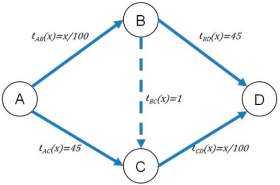
Figure 1.
The simple network used to simulate the effect of cognitive agents and demonstrate Braess Paradox. By adding an edge (which should intuitively help) a negative impact on all users of a congested network can be observed. The latency function l of each edge with respect to the number of agents on the edge x is given accordingly.
The Braess Paradox involves a non-intuitive outcome, associated with a traffic network, like that given in Figure 1. For this network, all original road segments (non-dashed edges) suffer increasing congestion as traffic flow increases. In order to simulate traffic on the original network we assume 4000 agents traveling from node A to node D along the given edges. Considering the original network without the additional edge eBC the players in the game will behave as players in a non-cooperative game. Hence, 2000 agents will take the path P1 = {A,B,D} and the remaining 2000 agents choose path P2 = {A,C,D} (see the left hand side of Figure 2). The given result is a flow at Nash equilibrium [25,26,27,28], which indicates that each agent is behaving “greedily”, without regard to the overall cost of travel on the network. Hence, each player travels along the minimum latency path currently available, with respect to the flow created by the other players. If a flow is at Nash equilibrium for an instance (G,r,l) assuming and with then all used si − ti paths have equal total latency. In the example employed here, the overall latency (cost of flow) C(f) equals 260,000 units (or 65 units of delay per agent). If the additional edge with high capacity (i.e., low latency lBC = 1) is added to the network, a flow at Nash equilibrium exists (assuming a non-cooperative game). The flow results in the following situation: All 4000 agents take the path P3 = {A,B,C,D} (see the right hand side of Figure 2, indicated by the red colored edges). The unique flow at equilibrium has a total cost C(f) which equals 324,000 units (or 81 units of delay per agent) [7,13,26,29]. Therefore, adding an additional edge and associated capacity can actually impede traffic flow rather than improve traffic flow, given that the agents act in a non-cooperative manner. This is an instance of Braess paradox.
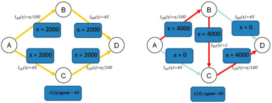
Figure 2.
Nash equilibrium flow and corresponding cost per agent C(f)/agent = 65 in the original network (left), and Nash flow after insertion of a high capacity edge (right). After adding the high capacity edge to the network, the total cost per agent C(f)/agent = 81, which is higher than in the original network.
Methodology to Evaluate the Effects of Cognitive Agents
To evaluate the effect of cognitive agents on Braess Paradox, we first introduce the concept of cognitive agents used in this work. After that, the evaluation approach is highlighted, which will incorporate varying levels of selfishness and uncertainty of travel times of the available paths from node A to D.
As opposed to non-cooperative games, where agents act in a strictly selfish manner, the approach presented here is comprised of cognitive agents. These agents are capable of making their own decisions based on their perceptions of the environment in which they act [30,31]. The concept of cognitive agents has been applied to wayfinding in built environments [32,33,34,35], and thus seems appropriate for traffic simulations as well. Hence, the agents in this work are able to make their own decisions while acting in the traffic network. In this work the reason for an agent’s decision is not a research focus, hence we just include simple cognitive abilities of the agent. Any agent is able to perceive the network status, i.e., congestion and latency, of a certain path (say by means of traffic news on a radio or by a navigation aid). In addition, an agent can decide their own action and choose a specific path to travel from node A to D. Therefore, the behavior of an agent has an effect on the other agents in terms of latency (and travel time). Of significant importance here is the fact that an agent’s decision does not necessarily have to be purely selfish, i.e., an agent may choose a path with a perceived higher latency (longer travel time), for whatever reason. Possible justifications for that behavior could be in personal preferences regarding the route choice, past experience that the route seems to be low in latency, toll roads/taxes (e.g., Reference [36]), or assumptions that the agent has regarding the behavior of other agents in terms of prospective memory [37].
In order to evaluate the effect of non-selfish behavior, different levels of selfishness are employed. This is represented by a parameter of non-selfishness probability PNS. The values of the parameter can range from 0 to 100, where 0 indicates that all decisions taken are selfish and 100 assumes that all decisions taken are of non-selfish nature. Usually probability levels have values from 0 to 1. In this paper, we use probability values multiplied by the factor 100, for the sake of readability. A PNS value of 50 means that there is a 50% probability that the decision of an agent will be non-selfish. Thus, the agents in the simulation may have selfish and non-selfish behavior. A non-selfish decision means, that the agent will not take the “obvious” faster path P3 = {A,B,C,D}, but chooses one of the “slower” paths P1 or P2, for whatever reasons. In order to evaluate the effect of non-selfish behavior, we have varied an agent’s probabilities of non-selfish decisions, from 0 to 100 in 5-unit steps—i.e., 0, 5, 10, …, 100.
Because agents in a traffic environment do not necessarily have accurate information on the status of traffic network, as discussed in Section 1. Therefore, we include an uncertainty factor for travel times in our approach, as this fact leads to a certain degree of uncertainty when making decisions. In order to evaluate the influence of varying levels of uncertainty on the Braess Paradox and the group of agents, we added uncertainty in latency and travel time information, denoted as ∆t, to the path P3 = {A,B,C,D} in the network. Hence, the total latency with uncertainty at P3 is denoted as C0(f). The calculation of C0(f) is defined in Equation (2),
where is a randomized positive number of the closed interval [0,∆t]. The ∆t is assigned a value ranging from 0 to 100 in 10-unit steps—i.e., 0, 10, 20, …, 100, according to the level of uncertainty that is applied in a specific test simulation.
We have evaluated the impact of various levels of selfishness of the decisions of cognitive agents under varying levels of latency uncertainty by simulating the group of cognitive agents in traveling from the origin and the destination. For each combination of level of non-selfishness PNS and uncertainty applied to latency of P3, 5000 simulation runs were performed (see Figure 3). In every simulation run 4000 agents have to travel from node A to node D, where they have to make decisions on the route taken based upon their cognitive and decision abilities. Overall, there are 231 combinations of P(NS) and ∆t. Given 5000 simulations for each distinct combination, there are 1,155,000 simulation runs. For each test run, we collected the following result variables: Total latency C0(f), the number of agents traversing edge eAB, the number of agents traversing edge eBD, the number of agents traversing edge eAC, the number of agents traversing edge eCD, the number of agents traversing edge eBC, and the number of selfish and non-selfish decisions made. For each distinct combination of ∆t and P(NS) the variables collected in each of the 5000 simulation runs were statistically analyzed. Hence, the mean value, the standard deviation and variance of each result variable for each combination of ∆t and PNS was calculated.
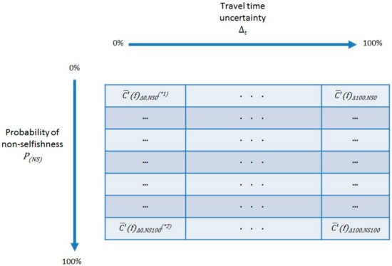
Figure 3.
Overview of the methodology to quantify the impact of cognitive agents, levels of selfishness and uncertainty on routing for a group of agents.
4. Experimental Results
This section presents the results of the evaluation approach highlighted in the previous section. The computational results are given in respective tables, elaborating on the effect of cognitive agents with respect to the experiment settings. The results were obtained using the Repast Simphony framework [38].
In Figure 3, the variable name for total latency value represents various levels of non-selfishness and travel time uncertainty. For example denotes the total latency value that occurs when the uncertainty level is 10 and the non-selfishness probability is set at 100. This means that represents delay incurred when the uncertainty in travel is at its lowest and when all agents’ decisions are selfish. The superscript (∗1) denotes that the additional edge BC is used, and superscript of (∗2) denotes that the edge BC is not used. This means that , marked with (∗2), denotes C(f) of the flow at Nash equilibrium without edge BC.
Our evaluation starts with the calculation of C(f) of the Nash flow on the original network i.e., without extra edge—and Ce(f) of the Nash flow of the extended network—i.e., with edge BC. Based on these “anchors”, the variable conditions of uncertainty of travel times and variable probability levels of non-selfishness were tested. The calculation of C(f) and Ce(f) is done according to the methodology mentioned in Section 3.1. Therefore, a non-cooperative game is created and evaluated until no agent can improve their individual situation by changing their behavior. Hence, C(f) results in 65 latency units per agent traveling from A to D, where 2000 agents traverse the edges AB-BD and the other 2000 agents choose AC-CD. For the network with the extra edge BC (having low latency) Ce(f) results in 81 units of latency per agent. In this case all 4000 agents traverse the edges AB-BC-CD. This paradox, of higher latency values due to an extra high capacity edge, is described in literature as Braess Paradox (e.g., Reference [8]).
In Table 1 the average latency values (i.e., total travel time over 5000 simulations) per agent are given for different levels of travel time uncertainty and probability of non-selfishness. The results indicate that the higher the level of uncertainty in terms of travel time ∆t is, the lower is the latency or delay per agent (given a fixed probability of non-selfishness P(NS)). This is depicted in Figure 4 and Table 1. Generally, the prior statement holds true except for the set of latency times highlighted in orange in Table 2. The highlighted values at a given P(NS) level are the lowest calculated values for given ∆t values. With increasing ∆t the values of increase. In Figure 5 the behavior of latency values for varying P(NS) with a given ∆t value is depicted (see Table 1 for numerical values). There, the latency values for ∆t values 0, 30, 60, 100 are depicted, showing decreasing latency values per agent with increasing P(NS). This monotonically decreasing behavior is present from P(NS) levels 0 to 90 (for ∆t ranging from 0–30), for P(NS) levels 0 to 85 (for ∆t ranging from 40–70), and for P(NS) levels 0 to 80 (for ∆t ranging from 80–100).

Table 1.
Average latency times of test runs for given values of varying ∆t and P(NS).
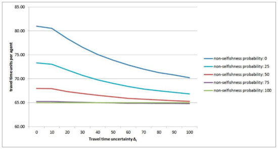
Figure 4.
Diagram showing the latency values per agent for given non-selfishness probabilities over varying travel time uncertainty values ∆t.
Table 2.
Lowest average latency times for varying ∆t and P(NS) are marked with orange colored numbers.
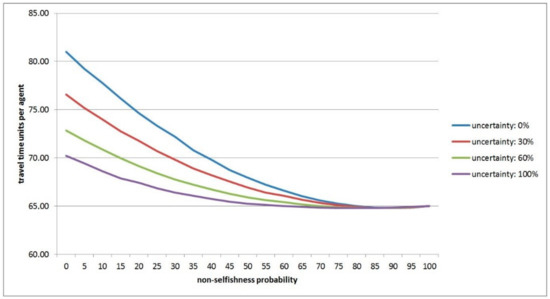
Figure 5.
Diagram showing the latency values per agent for given level of travel time uncertainty ∆t over varying probabilities of non-selfishness P(NS).
Both “anomalies”, depicted in Table 2, describe the fact that, when all agents follow the Nash flow without the edge BC, i.e., with latency C(f), then only a few agents choose to traverse edge BC. Thus, the agents act purely selfish by avoiding the edge BD with latency 45, which reduces latency for the agents (65 units verses 20 + 1 + (20 + x)/100 where x denotes the number of agents traversing edge BC). Hence, in this particular experiment setting a small number of agents in traversing edge BC can reduce the average latency per agent, which is depicted in Figure 4 and Figure 5 and Table 2.
In order to justify the latency values of Table 1—we show the number of agents traversing the respective edges in Appendix A Table A1 for edges AB and CD, and in Appendix A Table A2 for edges BD and AC. Appendix A Table A3 lists the number of agents traversing edge BC. These numbers are the basis for calculating the latency values given in Table 1 in conjunction with the latency functions given in Section 3.
In order to evaluate the stability in the number of agents traversing a certain edge the absolute standard deviation values and coefficient of variation have been computed. The coefficient of variation for edges AB and CD is between 0% and 31%, showing the highest variation coefficients at P(NS) values from 50 to 65 across all ∆t levels. In contrast to those numbers, the coefficient of variation for edges BD and AC are in the range between 8% and 395%, having decreasing coefficients of variation with higher P(NS) levels—except for P(NS) = 0. Hence, within the conducted test runs the standard deviation of edges BD and AC show higher values in comparison to AB and CD especially at low P(NS) and ∆t values. This is due to the fact that at low P(NS) and ∆t values edges BD and AC are not traversed by many agents, as most follow the path P3 = {A,B,C,D}. The coefficient of variation for edge BC ranges between 0% and 401% showing a high influence of P(NS) levels—i.e., increasing P(NS) leads to increasing variation.
In general, the coefficient of variation values reveals situations (i.e., distinct combinations of ∆t and P(NS)) which are volatile. Volatility in this context indicates test runs with high standard deviations, which in turn are unstable in terms of the number of traversing agents. Hence, a forecast or simulation of such situations is hardly possible, due to the variability of the system itself. For the experimental settings in this paper the edges AB and CD have an average coefficient of variation of 16% which is lower than the average coefficient of variation for edges BD and AC (53%). Hence, we can assume that the number of traversing agents of AB and CD are considered more stable than on AC and BD. For low ∆t values and low P(NS) levels coefficient of variation for edges AC and BD show especially high volatility due to the fact that the number of agents traversing these edges is low. The edge BC also shows unstable behavior in the test runs where the path P3 is seldom traversed.
The influence of the two variables ∆t and P(NS) on the average travel time per agent is also worth evaluating. In general, both variables have an influence on per agent, while P(NS) has a greater impact on per agent, than ∆t. This is justified by the numerical values given in Table 1, and by the correlation coefficients given in Table 3 and Table 4. In the tables the dependence of the latency values on the variables ∆t and P(NS) is given, where Table 4 indicates that P(NS) has higher impact on the values due to higher correlation coefficients in comparison to Table 3.
Table 3.
Correlation % between for given ∆t levels and P(NS), which indicates the dependence of travel delay on the uncertainty in travel information.
Table 4.
Correlation % between for given P(NS) levels and ∆t, which indicates the dependence between travel delay and the probability of selfishness.
On a global level the results reveal that the fastest route for an individual (i.e., shortest path in terms of travel time) does not necessarily have to be the fastest route for a group of people and for the individual itself, with respect to a defined network with latency functions. This is due to the behavior of other agents of the group and the latency due to the traffic volume on each edge, which is mentioned in Roughgarden [7]. Braess [8] and Roughgarden et al. [26] assume that each agent in the routing game acts in a strictly selfish manner, which results in the Braess Paradox. Therefore, if any player in a traffic situation would be equipped with a navigation system and would strictly follow the instructions of the navigation device the Braess Paradox is likely to occur. Thus, each member of the group travels with higher latency than without an extra high-capacity road present in the network. Roughgarden [7] mentions that the Price of Anarchy in networks with linear latency functions is at most 4/3. Of particular interest is that individual shortest paths do not necessarily lead to an “optimal” flow in the network if everyone acts selfish.
Nevertheless, if we consider real-world situations where agents in a network have uncertain information on the status of the network, they may act differently. Therefore, agents can make non-selfish decisions and take the longer path in terms of latency due to their preferences or their assumptions/view/information on the traffic situation. This behavior reduces the latency in the network, which is depicted in Table 1 and Table 2. Thus, in situations where a small number of agents travel on P3 the travel latency per agent is actually lower than in the network without the extra edge (see Figure 4 and Figure 5 and Table 1 and Table 2).
In that context, there is a possible impact on an Intelligent Transportation System (ITS) that tries to influence the decisions of agents which would result in an “optimal” flow. This could be realized by edge removal or with a special tax applied to high-capacity roads (see Reference [36]) or with “recommendations” for agents delivered by the navigation system. In addition, an agent could get rewards for taking detours (i.e., the longer path in terms of travel time). In Reference [36] the authors argue that the maximum benefit of taxes in networks with linear latency functions is 4/3, and with arbitrary latency functions is n/2, where n denotes the number of nodes in the network. The results here suggest that an approach to provide the agents in a traffic network with recommendations for the “optimal” paths that lead to the least global traffic latency, could easily be comprised by real-time communications that are directed to navigation systems (e.g., by utilizing the traffic message channel).
5. Conclusions and Future Work
This paper presents an analysis on the effect of cognitive agents on selfish routing in the context of a street network with a latency function on each edge. In contrast to the concept of a purely selfish routing problem, which is based upon the assumption of a non-cooperative game and strictly selfish agents [7,26], we consider cognitively enabled agents that can act in an environment with a given level of uncertainty associated with the status of the network in terms of latency information. In addition, each player in the system is able to act in both selfish and non-selfish ways, in contrast to a system with strictly selfish agents.
5.1. Crititcal Discussion of Obtained Results
The simulation environment consists of a network with linear latency functions and a group of 4000 agents that have to travel from an origin node to a destination node, by choosing amongst three different paths in the network. The network is defined in such a way that the Braess Paradox exists. The results indicate that both non-selfish behavior, and the uncertainty of traffic information (in terms of latency along a path), have an impact on overall travel time. The simulation results show that non-selfish decisions help to decrease the overall latency. While non-selfishness and uncertainty both have an influence on the total latency, non-selfish decisions taken by agents have a greater impact on latency than travel time uncertainty.
Of particular interest is the reduction of latency because of the travel time uncertainty, which might not be intuitive. As agents acting in the traffic network may have a “blurred” view of the network status ahead of them. As this issue affects the decision of each agent, having inaccurate information on, for example the current latency in the network, some agents might make “wrong” decisions that might not fit their chosen strategy, just because they have the wrong information. These situations may lead to some kind of distrust and dissatisfaction of real drivers. Thus, accurate, timely information on the status of the traffic network may be helpful for agents to come up with an appropriate route decision. In addition, Kattan et al. [10] conclude that agents having accurate and identical information from different information outlets are more likely to comply to the suggestions of a traffic management system.
In general, it can be observed that the fastest route for an individual does not correspond with the fastest route for a group of people, if all individuals follow their individual fastest route—with respect to a given network with linear latency functions. Hence, agents acting on a traffic network and strictly following route suggestions of e.g., a navigation systems (without TMC), may result in higher latency or travel time for all agents. If the majority of agents act in a non-selfish manner (i.e., taking what appears to be the slower path), while only some take the fast path, a low total latency can be observed, even slightly lower than the latency of the original network (65 min latency verses 64.8 mins latency).
5.2. Future Work and Connection to ITS
In the context of ITS, the results of this paper can be of interest, due to the fact that guidance systems could influence the decisions of agents which can result in an “optimal” traffic flow. In order to influence the traffic flow, the literature suggests the application of tolls on certain edges [36] or to remove certain edges of the network [39]. In addition, traffic could be influenced by rewarding agents for traversing longer paths in terms of travel time. Nevertheless, Kattan et al. [10] suggest that a proper information provision is a crucial part for “influencing” agents’ decisions. According to their work drivers that obtain the same information from different information outlets are more likely to comply to the suggestions.
Future work includes the evaluation of cognitive agents in larger networks with arbitrary latency functions. In addition, the concept of predictive memory could be applied to agents—currently being utilized in Personal Information Management (e.g., Reference [37]). In addition, predictive memory—a concept based on the recognition-prediction framework—could enable agents to learn from previous experiences [40,41]. Agents are then capable of making assumptions regarding the behavior of other agents and they can gradually build up and act upon a set of past experiences.
Author Contributions
J.S. contributed the research idea, and developed the theory in conjunction with R.L.C., and conducted the implementation of the experiments. J.S. wrote the initial manuscript which was edited by R.L.C. R.L.C. contributed to the research questions, the theory and critical conclusions. R.L.C. substantially helped J.S. to edit and revise the manuscript.
Funding
This research received no external funding.
Acknowledgments
Supported by TU Graz Open Access Publishing Fund.
Conflicts of Interest
The authors declare no conflict of interest.
Appendix A. Supplementary Results
Table A1.
Average number of agents traversing edge AB and CD for given values of ∆t and P(NS).
Table A1.
Average number of agents traversing edge AB and CD for given values of ∆t and P(NS).
| Agents Traversing Edge AB and CD | |||||||||||
|---|---|---|---|---|---|---|---|---|---|---|---|
| Travel Time Uncertainty ∆t | |||||||||||
| P(NS) | 0 | 10 | 20 | 30 | 40 | 50 | 60 | 70 | 80 | 90 | 100 |
| 0 | 4000 | 3974.81 | 3849.15 | 3734.76 | 3632.05 | 3547.62 | 3469.37 | 3401.86 | 3339.55 | 3295.05 | 3241.06 |
| 5 | 3900.07 | 3879.95 | 3758.69 | 3641.37 | 3547.75 | 3461.11 | 3384.27 | 3321.4 | 3257.16 | 3200.6 | 3162.78 |
| 10 | 3811.04 | 3774.2 | 3663.04 | 3555.4 | 3460.76 | 3379.4 | 3300.79 | 3242.36 | 3167.76 | 3120.97 | 3073.99 |
| 15 | 3708.08 | 3679.9 | 3580.8 | 3461.63 | 3376.74 | 3287.77 | 3215.32 | 3155.59 | 3101.99 | 3033.97 | 2986.3 |
| 20 | 3604.07 | 3583.16 | 3481.59 | 3381.52 | 3298.92 | 3199.16 | 3132.09 | 3080.07 | 3010.67 | 2959.26 | 2923.24 |
| 25 | 3505.82 | 3482.06 | 3386.4 | 3286.22 | 3196.58 | 3120.97 | 3048.38 | 2983.14 | 2933.44 | 2886.59 | 2838.81 |
| 30 | 3416.31 | 3384.71 | 3280.88 | 3199.04 | 3115.95 | 3046.93 | 2969.3 | 2922.98 | 2861.46 | 2809.34 | 2767.17 |
| 35 | 3294.03 | 3280.85 | 3192.62 | 3107.43 | 3042.72 | 2952.77 | 2894.61 | 2841.55 | 2794.96 | 2743.55 | 2707.56 |
| 40 | 3201.92 | 3176.84 | 3097.61 | 3025.9 | 2952.37 | 2879.66 | 2823.73 | 2775.24 | 2720.1 | 2675.26 | 2636.41 |
| 45 | 3089.87 | 3088.58 | 3009.95 | 2943.63 | 2872.17 | 2815.76 | 2748.1 | 2697.71 | 2652.49 | 2612.29 | 2569.12 |
| 50 | 2995.9 | 2994.26 | 2912.51 | 2852.01 | 2791.12 | 2731.5 | 2671.15 | 2629.46 | 2587.19 | 2548.21 | 2507.01 |
| 55 | 2898 | 2892.6 | 2827.96 | 2769.3 | 2724.01 | 2660.53 | 2608.99 | 2570.34 | 2526.3 | 2485.34 | 2460.01 |
| 60 | 2800.92 | 2798.16 | 2743.45 | 2702.34 | 2646.85 | 2587.73 | 2548.51 | 2503.55 | 2465.33 | 2432.68 | 2401.98 |
| 65 | 2694.2 | 2694.99 | 2658.81 | 2615.55 | 2568.78 | 2519.65 | 2478.97 | 2436.63 | 2404.11 | 2375.98 | 2348.21 |
| 70 | 2594.52 | 2596.72 | 2566.77 | 2525.5 | 2482.91 | 2443.28 | 2405.1 | 2371.54 | 2340.83 | 2315.53 | 2291.25 |
| 75 | 2500.25 | 2497.14 | 2469.29 | 2441.55 | 2402.34 | 2366.42 | 2336.04 | 2310.01 | 2282.15 | 2260.36 | 2241.7 |
| 80 | 2401.09 | 2394.62 | 2381 | 2353.58 | 2323.59 | 2292.75 | 2273.31 | 2250.37 | 2222.16 | 2205.35 | 2191.58 |
| 85 | 2296.75 | 2295.48 | 2290.35 | 2267.5 | 2242.06 | 2224.12 | 2205.9 | 2184.36 | 2166.27 | 2153.98 | 2141.78 |
| 90 | 2196.33 | 2202.09 | 2194.23 | 2174.59 | 2158.42 | 2150.37 | 2131.68 | 2118.38 | 2111.17 | 2100.74 | 2091.57 |
| 95 | 2094.3 | 2104.05 | 2092.21 | 2086.44 | 2081.78 | 2072.18 | 2065.88 | 2059.27 | 2054.71 | 2048.08 | 2043.54 |
| 100 | 2000 | 2000 | 2000 | 2000 | 2000 | 2000 | 2000 | 2000 | 2000 | 2000 | 2000 |
Table A2.
Average number of agents traversing edge BD and AC for given values of ∆t and P(NS).
Table A2.
Average number of agents traversing edge BD and AC for given values of ∆t and P(NS).
| Agents Traversing Edge BD and AC | |||||||||||
|---|---|---|---|---|---|---|---|---|---|---|---|
| Travel Time Uncertainty ∆t | |||||||||||
| P(NS) | 0 | 10 | 20 | 30 | 40 | 50 | 60 | 70 | 80 | 90 | 100 |
| 0 | 0 | 25.2 | 150.85 | 265.25 | 367.96 | 452.39 | 530.65 | 598.17 | 660.47 | 705 | 758.97 |
| 5 | 99.93 | 120.06 | 241.32 | 358.65 | 452.26 | 538.91 | 615.76 | 678.64 | 742.88 | 799.45 | 837.27 |
| 10 | 188.96 | 225.81 | 336.97 | 444.62 | 539.27 | 620.64 | 699.24 | 757.69 | 832.29 | 879.08 | 926.07 |
| 15 | 291.92 | 320.09 | 419.22 | 538.4 | 623.3 | 712.27 | 784.74 | 844.47 | 898.08 | 966.08 | 1013.76 |
| 20 | 395.93 | 416.84 | 518.42 | 618.52 | 701.13 | 800.9 | 867.97 | 920 | 989.38 | 1040.81 | 1076.82 |
| 25 | 494.18 | 517.94 | 613.63 | 713.82 | 803.47 | 879.08 | 951.68 | 1016.92 | 1066.64 | 1113.47 | 1161.24 |
| 30 | 583.68 | 615.29 | 719.14 | 800.99 | 884.09 | 953.13 | 1030.75 | 1077.09 | 1138.6 | 1190.71 | 1232.91 |
| 35 | 705.97 | 719.16 | 807.4 | 892.6 | 957.32 | 1047.28 | 1105.45 | 1158.51 | 1205.12 | 1256.52 | 1292.52 |
| 40 | 798.08 | 823.16 | 902.42 | 974.12 | 1047.68 | 1120.38 | 1176.34 | 1224.83 | 1279.97 | 1324.81 | 1363.66 |
| 45 | 910.13 | 911.42 | 990.07 | 1056.4 | 1127.87 | 1184.3 | 1251.96 | 1302.35 | 1347.58 | 1387.78 | 1430.94 |
| 50 | 1004.09 | 1005.74 | 1087.51 | 1148.02 | 1208.94 | 1268.55 | 1328.9 | 1370.62 | 1412.87 | 1451.87 | 1493.05 |
| 55 | 1102 | 1107.41 | 1172.06 | 1230.75 | 1276.05 | 1339.54 | 1391.08 | 1429.74 | 1473.78 | 1514.74 | 1540.07 |
| 60 | 1199.08 | 1201.85 | 1256.56 | 1297.71 | 1353.2 | 1412.33 | 1451.55 | 1496.53 | 1534.73 | 1567.4 | 1598.09 |
| 65 | 1305.8 | 1305.01 | 1341.21 | 1384.49 | 1431.27 | 1480.41 | 1521.1 | 1563.45 | 1595.96 | 1624.09 | 1651.85 |
| 70 | 1405.47 | 1403.29 | 1433.25 | 1474.53 | 1517.13 | 1556.78 | 1594.95 | 1628.52 | 1659.21 | 1684.53 | 1708.8 |
| 75 | 1499.75 | 1502.86 | 1530.74 | 1558.48 | 1597.72 | 1633.63 | 1664.01 | 1690.05 | 1717.91 | 1739.7 | 1758.34 |
| 80 | 1598.9 | 1605.38 | 1619.01 | 1646.45 | 1676.45 | 1707.29 | 1726.74 | 1749.67 | 1777.88 | 1794.69 | 1808.45 |
| 85 | 1703.25 | 1704.52 | 1709.66 | 1732.52 | 1757.97 | 1775.93 | 1794.13 | 1815.68 | 1833.76 | 1846.06 | 1858.25 |
| 90 | 1803.68 | 1797.91 | 1805.78 | 1825.43 | 1841.59 | 1849.65 | 1868.34 | 1881.64 | 1888.85 | 1899.29 | 1908.44 |
| 95 | 1905.7 | 1895.96 | 1907.78 | 1913.57 | 1918.23 | 1927.83 | 1934.13 | 1940.75 | 1945.3 | 1951.93 | 1956.47 |
| 100 | 2000 | 2000 | 2000 | 2000 | 2000 | 2000 | 2000 | 2000 | 2000 | 2000 | 2000 |
Table A3.
Average number of agents traversing edge BC for given values of ∆t and P(NS).
Table A3.
Average number of agents traversing edge BC for given values of ∆t and P(NS).
| Agents Traversing Edge BC | |||||||||||
|---|---|---|---|---|---|---|---|---|---|---|---|
| Travel Time Uncertainty ∆t | |||||||||||
| P(NS) | 0 | 10 | 20 | 30 | 40 | 50 | 60 | 70 | 80 | 90 | 100 |
| 0 | 4000 | 3949.61 | 3698.31 | 3469.51 | 3264.09 | 3095.23 | 2938.71 | 2803.68 | 2679.09 | 2590.05 | 2482.09 |
| 5 | 3800.14 | 3759.89 | 3517.36 | 3282.72 | 3095.49 | 2922.2 | 2768.52 | 2642.76 | 2514.28 | 2401.15 | 2325.51 |
| 10 | 3622.09 | 3548.39 | 3326.07 | 3110.78 | 2921.49 | 2758.76 | 2601.55 | 2484.67 | 2335.47 | 2241.89 | 2147.92 |
| 15 | 3416.16 | 3359.81 | 3161.58 | 2923.23 | 2753.44 | 2575.5 | 2430.58 | 2311.12 | 2203.9 | 2067.89 | 1972.54 |
| 20 | 3208.14 | 3166.32 | 2963.17 | 2763 | 2597.78 | 2398.26 | 2264.12 | 2160.07 | 2021.29 | 1918.45 | 1846.42 |
| 25 | 3011.63 | 2964.12 | 2772.76 | 2572.4 | 2393.1 | 2241.89 | 2096.7 | 1966.23 | 1866.79 | 1773.12 | 1677.57 |
| 30 | 2832.63 | 2769.42 | 2561.74 | 2398.05 | 2231.86 | 2093.81 | 1938.55 | 1845.89 | 1722.86 | 1618.63 | 1534.26 |
| 35 | 2588.06 | 2561.69 | 2385.22 | 2214.83 | 2085.4 | 1905.49 | 1789.16 | 1683.04 | 1589.84 | 1487.03 | 1415.04 |
| 40 | 2403.84 | 2353.68 | 2195.19 | 2051.78 | 1904.69 | 1759.28 | 1647.39 | 1550.42 | 1440.13 | 1350.45 | 1272.75 |
| 45 | 2179.75 | 2177.16 | 2019.88 | 1887.23 | 1744.3 | 1631.47 | 1496.15 | 1395.37 | 1304.91 | 1224.51 | 1138.18 |
| 50 | 1991.81 | 1988.52 | 1824.99 | 1703.99 | 1582.17 | 1462.94 | 1342.25 | 1258.84 | 1174.32 | 1096.34 | 1013.95 |
| 55 | 1796.01 | 1785.18 | 1655.9 | 1538.55 | 1447.95 | 1320.99 | 1217.91 | 1140.6 | 1052.52 | 970.6 | 919.93 |
| 60 | 1601.83 | 1596.3 | 1486.89 | 1404.63 | 1293.66 | 1175.4 | 1096.96 | 1007.02 | 930.6 | 865.28 | 803.88 |
| 65 | 1388.41 | 1389.98 | 1317.6 | 1231.07 | 1137.51 | 1039.24 | 957.87 | 873.18 | 808.16 | 751.88 | 696.36 |
| 70 | 1189.05 | 1193.43 | 1133.51 | 1050.97 | 965.78 | 886.51 | 810.15 | 743.02 | 681.62 | 631 | 582.46 |
| 75 | 1000.51 | 994.29 | 938.55 | 883.07 | 804.62 | 732.79 | 672.03 | 619.96 | 564.24 | 520.66 | 483.36 |
| 80 | 802.19 | 789.24 | 761.99 | 707.13 | 647.15 | 585.46 | 546.57 | 500.7 | 444.28 | 410.66 | 383.13 |
| 85 | 593.49 | 590.96 | 580.69 | 534.98 | 484.1 | 448.19 | 411.77 | 368.68 | 332.51 | 307.92 | 283.53 |
| 90 | 392.65 | 404.18 | 388.46 | 349.16 | 316.83 | 300.73 | 263.34 | 236.75 | 222.32 | 201.45 | 183.13 |
| 95 | 188.59 | 208.09 | 184.43 | 172.87 | 163.55 | 144.35 | 131.74 | 118.52 | 109.41 | 96.15 | 87.06 |
| 100 | 0 | 0 | 0 | 0 | 0 | 0 | 0 | 0 | 0 | 0 | 0 |
References
- Montello, D.R. Navigation. In The Cambridge Handbook of Visuospatial Thinking; Shah, P., Miyake, A., Eds.; Cambridge University Press: Cambridge, UK, 2005; pp. 257–294. [Google Scholar]
- Kamburowski, J. A note on the stochastic shortest route problem. Oper. Res. 1985, 33, 696–698. [Google Scholar] [CrossRef]
- Kaufman, D.E.; Smith, R.L. Fastest paths in time-dependent networks for IVHS application. IVHS J. 1993, 1, 1–11. [Google Scholar]
- Orda, A.; Rom, R. Minimum weight paths in time-dependent network. Networks 1991, 21, 295–320. [Google Scholar] [CrossRef]
- Ziliaskopoulos, A.; Mahmassani, H.S. Time-dependent shortest path algorithm for realtime intelligent vehicle highway system applications. Transp. Res. Rec. 1993, 1408, 295–320. [Google Scholar]
- Ding, B.; Yu, J.X.; Qin, L. Finding time-dependent shortest paths over large graphs. In Proceedings of the 11th International Conference on Extending Database Technology: Advances in Database Technology, Nantes, France, 25–29 March 2008; ACM: New York, NY, USA, 2008; pp. 205–216. [Google Scholar]
- Roughgarden, T. Selfish Routing and the Price of Anarchy; The MIT Press: Cambridge, MA, USA, 2005. [Google Scholar]
- Braess, D. Ueber ein Paradoxon aus der Verkehrsplanung. Unternehmensforschung 1968, 12, 258–268. [Google Scholar]
- Wazestats.com. Maximum of Wazers per Million Citizens at 2018/05/02. Available online: http:// http://wazestats.com (accessed on 22 August 2018).
- Kattan, L.; Habib, K.M.N.; Tazul, I.; Shahid, N. Information provision and driver compliance to advanced traveller information system application: Case study on the interaction between variable message sign and other sources of traffic updates in Calgary, Canada. Can. J. Civ. Eng. 2011, 38, 1335–1346. [Google Scholar]
- Meyer, M.D.; Miller, E.J. Urban Transportation Planning: A Decision-Oriented Approach; McGraw-Hill: Boston, MA, USA, 2001; ISBN 0-07-242332-3. [Google Scholar]
- McNally, M.G. The Four-Step Model. In Handbook of Transport Modelling; Emerald Insight Publishing: Bingley, West Yorkshire, UK, 2007; pp. 35–53. [Google Scholar]
- Wardrop, J.G. Road paper. Some theoretical aspects of road traffic research. In ICE Proceedings: Engineering Divisions; ICE Virtual Library: London, UK, 1952; Volume 1, pp. 325–362. [Google Scholar]
- Myerson, R.B. Game Theory: Analysis of Conflict; Harvard University Press: Cambridge, MA, USA, 1991. [Google Scholar]
- Nash, J. Non-Cooperative Games. Ann. Math. 1951, 54, 286–295. [Google Scholar] [CrossRef]
- Ford, L.R., Jr.; Fulkerson, D.R. Flows in Networks; Princeton University Press: Princeton, NJ, USA, 2010; ISBN 0-691-14667-5. [Google Scholar]
- Goldberg, A.V.; Tardos, E.; Tarjan, R.E. Network Flow Algorithms. In Paths, Flows and VLSI-Layout; Korte, B., Lovasz, L., Prömel, H.J., Schrijver, A., Eds.; Springer Verlag: Berlin, Germany, 1990; pp. 101–164. [Google Scholar]
- Tucker, A.W. A Two-Person Dilemma. Unpublished Notes. 1950. Available online: http://www.rasmusen.org/x/images/pd.jpg (accessed on 22 August 2018).
- Papadimitriou, C. Algorithms, games, and the internet. In Proceedings of the Thirty-Third Annual ACM Symposium on Theory of Computing, Crete, Greece, 6–8 July 2001; ACM: New York, NY, USA, 2001; pp. 749–753. [Google Scholar]
- Zhang, K.; Nie, Y.M. Mitigating the impact of selfish routing: An optimal-ratio control scheme (ORCS) inspired by autonomous driving. Transp. Res. Part C Emerg. Technol. 2018, 87, 75–90. [Google Scholar] [CrossRef]
- Christodoulou, G.; Mehlhorn, K.; Pyrga, E. Improving the price of anarchy for selfish routing via coordination mechanisms. Algorithmica 2014, 69, 619–640. [Google Scholar] [CrossRef]
- Hasan, M.R.; Bazzan, A.L.; Friedman, E.; Raja, A. A multiagent solution to overcome selfish routing in transportation networks. In Proceedings of the 2016 IEEE 19th International Conference on Intelligent Transportation Systems (ITSC), Rio de Janeiro, Brazil, 1–4 November 2016; pp. 1850–1855. [Google Scholar]
- Cole, R.; Lianeas, T.; Nikolova, E. When Does Diversity of Agent Preferences Improve Outcomes in Selfish Routing? In Proceedings of the IJCAI, Stockholm, Sweden, 13–19 July 2018; pp. 173–179. [Google Scholar]
- Zhang, W.; He, Z.; Guan, W.; Ma, R. Selfish routing equilibrium in stochastic traffic network: A probability-dominant description. PLoS ONE 2017, 12, e0183135. [Google Scholar] [CrossRef] [PubMed]
- Friedman, E.J. Genericity and congestion control in selfish routing. In Proceedings of the 43rd IEEE Conference on Decision and Control, Nassau, Bahamas, 14–17 November 2004; Volume 5, pp. 4667–4672. [Google Scholar]
- Roughgarden, T.; Tardos, É. How bad is selfish routing? J. ACM 2002, 49, 236–259. [Google Scholar] [CrossRef]
- Frank, M. The Braess Paradox. Math. Program. 1968, 20, 283–302. [Google Scholar] [CrossRef]
- Steinberg, R.; Zangwill, W.I. The prevalence of Braess’ paradox. Transp. Sci. 1983, 17, 301–318. [Google Scholar] [CrossRef]
- Beckmann, M.; McGuire, C.; Winsten, C.B. Studies in the Economics of Transportation; Yale University Press: New Haven, CT, USA, 1956. [Google Scholar]
- Frank, A.U.; Bittner, S.; Raubal, M. Spatial and cognitive simulation with multi-agent systems. In Spatial Information Theory; Springer: Berlin, Germany, 2001; pp. 124–139. [Google Scholar]
- Russel, S.; Norvig, P. Artificial Intelligence—A Modern Approach; Prentice Hall International, Inc.: Upper Saddle River, NJ, USA, 1995. [Google Scholar]
- Raubal, M.; Worboys, M. A formal model of the process of wayfinding in built environments. In Spatial Information Theory. Cognitive and Computational Foundations of Geographic Information Science; Springer: Berlin, Germany, 1999; pp. 381–399. [Google Scholar]
- Raubal, M.; Egenhofer, M.J. Comparing the complexity of wayfinding tasks in built environments. Environ. Plan. B 1998, 25, 895–914. [Google Scholar] [CrossRef]
- Jonietz, D.; Kiefer, P. Uncertainty in Wayfinding: A Conceptual Framework and Agent-Based Model. In Proceedings of the 13th International Conference on Spatial Information Theory (COSIT 2017), L’Aquila, Italy, 4–8 September 2017; Clementini, E., Donnelly, M., Yuan, M., Kray, C., Fogliaroni, P., Ballatore, A., Eds.; Leibniz International Proceedings in Informatics (LIPIcs), Schloss Dagstuhl–Leibniz-Zentrum fuer Informatik: Dagstuhl, Germany, 2017; Volume 86, p. 15. [Google Scholar]
- Hoogendoorn, S.P.; Bovy, P.H. Pedestrian route-choice and activity scheduling theory and models. Transp. Res. Part B Methodol. 2004, 38, 169–190. [Google Scholar] [CrossRef]
- Cole, R.; Dodis, Y.; Roughgarden, T. How much can taxes help selfish routing? J. Comput. Syst. Sci. 2006, 72, 444–467. [Google Scholar] [CrossRef]
- Abdalla, A.; Frank, A.U. Personal geographic information management. In Proceedings of the Workshop on Cognitive Engineering for Mobile GIS (CEUR Workshop Proceedings), Belfast, ME, USA, 12 September 2011. [Google Scholar]
- North, M.J.; Collier, N.T.; Ozik, J.; Tatara, E.R.; Macal, C.M.; Bragen, M.; Sydelko, P. Complex adaptive systems modeling with Repast Simphony. Complex Adapt. Syst. Model. 2013, 1, 3. [Google Scholar] [CrossRef]
- Cole, R.; Dodis, Y.; Roughgarden, T. Pricing Networks with Selfish Routing; Department of Computer Science, Cornell University: Ithaca, NY, USA, 2003. [Google Scholar]
- Clark, A. Whatever next? Predictive brains, situated agents, and the future of cognitive science. Behav. Brain Sci. 2013, 36, 181–204. [Google Scholar] [CrossRef] [PubMed]
- Hawkins, J.; Blakeslee, S. On Intelligence: How a New Understanding of the Brain Will Lead to the Creation of Truly Intelligent Machines; MacMillan: Basingstoke, UK, 2007. [Google Scholar]


© 2018 by the authors. Licensee MDPI, Basel, Switzerland. This article is an open access article distributed under the terms and conditions of the Creative Commons Attribution (CC BY) license (http://creativecommons.org/licenses/by/4.0/).