Representative Band Selection for Hyperspectral Image Classification

Abstract

The high dimensionality of hyperspectral images (HSIs) brings great difficulty for their later data processing. Band selection, as a commonly used dimension reduction technique, is the selection of optimal band combinations from the original bands, while attempting to remove the redundancy between bands and maintain a good classification ability. In this study, a novel hybrid filter-wrapper band selection method is proposed by a three-step strategy, i.e., band subset decomposition, band selection and band optimization. Based on the information gain (IG) and the spectral curve of the hyperspectral dataset, the band subset decomposition technique is improved, and a random selection strategy is suggested. The implementation of the first two steps addresses the problem of reducing inter-band redundancy. An optimization strategy based on a gray wolf optimizer (GWO) ensures that the selected band combination has a good classification ability. The classification performance of the selected band combination is verified on the Indian Pines, Pavia University and Salinas hyperspectral datasets with the aid of support vector machine (SVM) with a five-fold cross-validation. By comparing the proposed IG-GWO method with five state-of-the-art band selection approaches, the superiority of the proposed method for HSIs classification is experimentally demonstrated on three well-known hyperspectral datasets.

1. Introduction

Remotely sensed hyperspectral data which is collected by hyperspectral sensors consist of hundreds of contiguous spectral bands with high resolutions [1,2]. Recent studies in remote sensing have shown that hyperspectral images (HSIs) have been successfully applied in precision agriculture, urban planning, environmental monitoring and various other fields [3,4,5,6]. One of the typical characteristics of an HSI is that it cannot only obtain the scene information in the two-dimensional space of the target image but can also acquire one-dimensional spectral information with a high resolution to characterize the physical property. However, the superiority of HSIs with high resolution occurs at the expense of their vast amount of data and their high-dimensionality property (often including hundreds of bands). Furthermore, the great deal of information can also deteriorate the accuracy of classification, due to the redundant and noisy bands [7,8]. Therefore, it is of great importance to introduce new dimensionality-reduction methods that readily utilize the information resources of HSIs.

A large number of dimensionality reduction (DR) approaches have been developed in the past decades [9,10,11,12,13,14,15,16,17,18,19,20]. The existing dimensionality reduction methods can be commonly partitioned into the two branches of feature/band extraction and feature/band selection. The former projects the original high-dimensional HSIs data into a lower-dimensional space to reduce the number of dimensions through various transformations [16]. Typical algorithms include locally linear embedding (LLE) [17], principal component analysis (PCA) [12,18], and locality preserving projection (LPP) [19]. A powerful moment distance method was proposed for hyperspectral analysis by using all bands or a subset of bands to detect the shape of the curve in vegetation studies [14]. Despite the favorable results that can be provided by these methods, the critical information is sometimes damaged after the destruction of the band correlation in the transformation of HSIs data [20]. Therefore, compared with the band selection approaches, these methods are not always the most optimal choices for dimensionality reduction.

As for the band selection method, the most informative and distinctive band subset is automatically selected from the original band space of the HSIs [21,22,23]. Briefly, band selection technology contains two key elements: the search strategy and the evaluation criterion function [24]. The former seeks the most discriminative band subset among all feasible subsets through an impactful search strategy, while the latter evaluates a score for each band subset that was selected from the original bands by a suitable criterion function.

The search strategy for the optimal subset is a crucial issue in band selection. One can traverse all combinations of band subsets to generate the optimal subset by an exhaustive search [25]. However, this method is inapplicable after considering the high dimensionality of hyperspectral data. To randomly select m bands out of the n original bands, there are n!/(n − m)!m! possible results. An extremely high computational cost could be paid for selecting the optimal band combination from all band combinations. Another method is to randomly search for the minimal reduction by metaheuristics [26].

The inspiration for the metaheuristics usually comes from nature. It is mainly reflected in three types [27]: physics-based (simulated annealing [28]), evolutionary-based (genetic algorithm [29]), and swarm-based (GWO [30], artificial bee colony [31], particle swarm optimization [32],). Notably, the swarm-based technique has been extensively investigated in order to seek out the global optimal band combination by using stochastic and bio-inspired optimization techniques. The GWO algorithm advocated by Mirjalili [30] is a novel evolutionary-based method and is capable of offering competitive results, in contrast with the other state-of-the-art metaheuristics algorithms. It has the advantages of a broader range of pre-search, simple operation and fast convergence [30]. It is advantageous for approximating the global optimal solution [33,34,35,36]. Medjahed et al. [33] first applied the GWO algorithm to search for the optimal band combination for HSIs classification. It can be seen from their work that the classification result was not satisfied.

With regards to evaluation criteria, each candidate band subset could be assessed by two different techniques: wrapper and filter [27]. In the wrapper-based method [27,37,38,39], the learning algorithm, as a predictor wrapped on the search algorithm, participates in the evaluation of the band subset during its search procedure, and the classification results are used as the evaluation criteria for the band subset. In Ma et al. [39], the three indices of classification accuracy, computing time and stability were used to construct the criteria for evaluation. Despite the attractive performance of the wrapper-based approach, unfortunately, an enormous computational burden would be triggered because a new model is invariably established to evaluate the current band subset at every turn during the search procedures [40].

The filter-based method evaluates a score for each band or band subset by measuring their inherent attributes that are associated with their class separability rather than a learning method (classification algorithm) [41]. Often, correlation criteria, distance or information entropy are taken as measurements [42]. As a direct criterion for similarity comparison, linear prediction (LP) jointly evaluates the similarity between a single band and multiple bands [43]. The Laplacian score (Lscore) criterion has been utilized to rank bands in order to reduce the search space and obtain the optimal band subset [44]. Mutual information (MI) has been extensively used over the years as the measurement criterion due to its nonlinear and nonparametric characteristics [20,23]. Trivariate mutual information (TMI) is different from the traditional MI-based criterion and takes the correlation among three variables (the class label and two bands) into account concurrently [45]. The semi-supervised band selection approach based on TMI and graph regulation (STMIGR) used a graph regulation term to select the informative features by unlabeled samples [45]. Based on Ward’s linkage and MI, a hierarchical clustering method was introduced to reduce the original bands [20]. This approach was termed WaLuMI. Maximum information and minimum redundancy (MIMR) defines a criterion that maximizes the amount of information for the selected band combination while removing redundant information [23]. The bands with low redundancy were selected by MI for HSIs classification in these methods. However, choosing a certain number of bands to minimize the correlation among them is a time-consuming optimization issue [46]. Information gain (IG), also known as the Kullback–Leibler divergence, can measure how much information the features could contribute to the classification. In a previous study [47], IG was applied to rank the text features to achieve text recognition. Intuitively, the features with larger IG values are considered informative and momentous contributions to classification. Koonsanit [48] proposed an integrated PCA and IG method for hyperspectral band selection that significantly reduced the computational complexity. Qian et al. [15] used IG as the similarity function to measure the similarity between the two bands, and then an AP clustering algorithm was used to cluster the initial band to select the optimal band subset.

Compared with the wrapper method, the filter-based method is independent of the subsequent learning algorithms during the band selection process and has the advantages of a low computational complexity and strong generalization capability [40,41]. However, there are still two issues that need to be addressed: (1) the representative bands can be quickly obtained in terms of the score of each band in the filter-based method, but the correlation between the selected bands may be high; (2) some bands show a significant and indispensable effect on HSIs classification when combined with other bands. However, their score may not be high, so they may be abandoned in error.

On the basis of the above analysis, it is highly necessary to develop a hybrid filter–wrapper feature selection method. In this paper, the filter method based on IG is designed to replace the predictor wrapped on the search algorithm in the wrapped method. The experimental results show that this attempt achieves a reasonable compromise between efficiency (computing time) and effectiveness (classification accuracy actualized by the selected bands).

Furthermore, inspired by the concept of the adaptive subspace decomposition approach (ASD) [49], an improved subspace decomposition approach has been newly defined. As described previously [49], the entire spectral bands were first partitioned into band subsets in line with the correlation coefficient of adjacent bands. Then, bands were selected from each subset according to the quantity of information or class separability. Nevertheless, ASD did not overcome the limitations of the traditional subspace decomposition method, which only used correlation coefficients to partition the band space. This leads to the problem that subspaces are difficult to partition because of their multiple minimum points. Thus, we suggest an improved subspace decomposition technique in which band space is decomposed by calculating the value of IG along with the visualization result of the HSIs spectral curve. Moreover, the selection of the same number of bands from each band subset ensures that each band subset makes the same contribution to the final classification results.

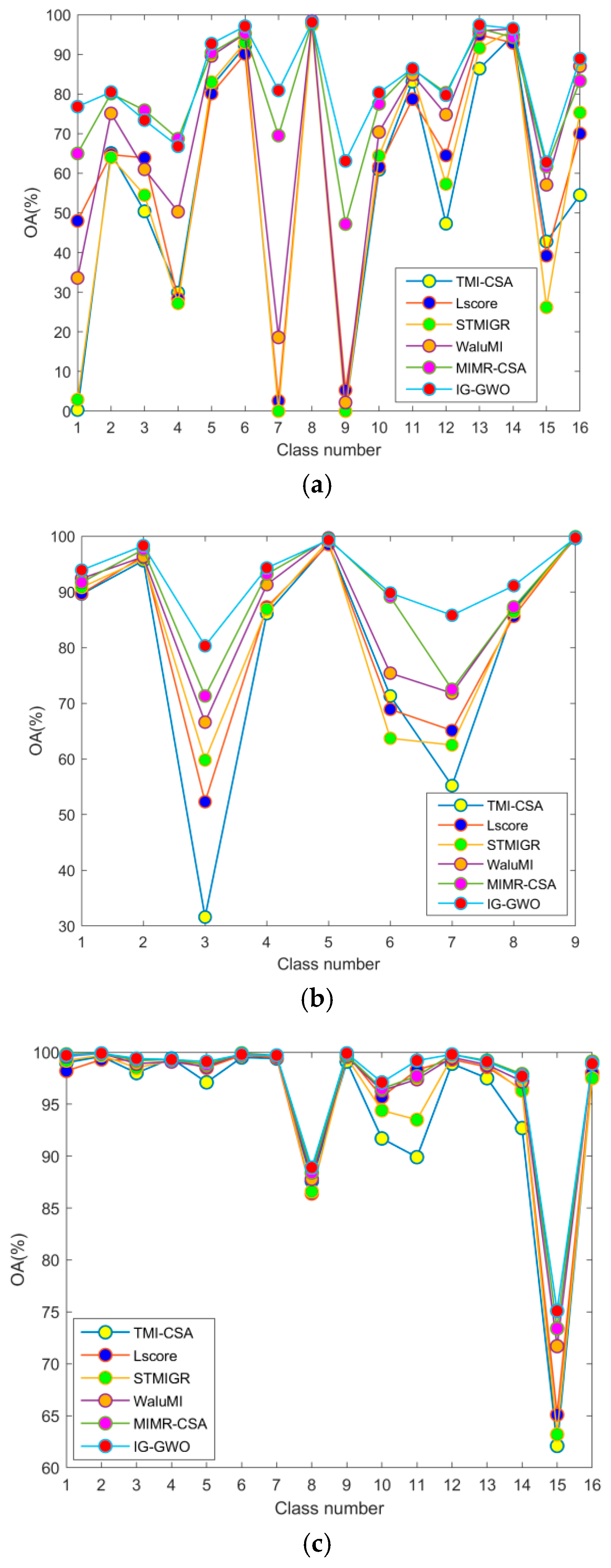
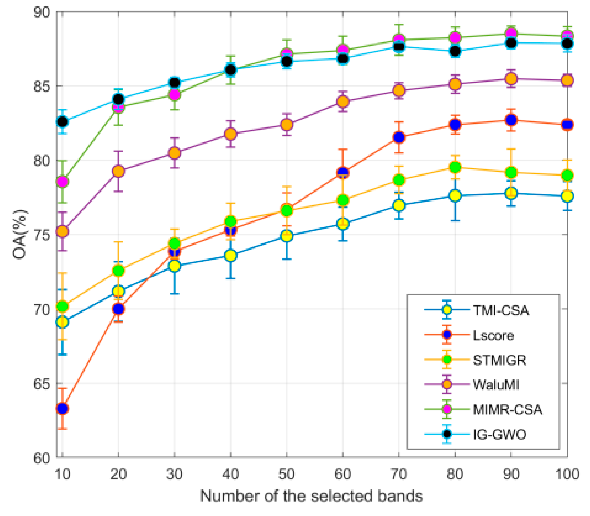
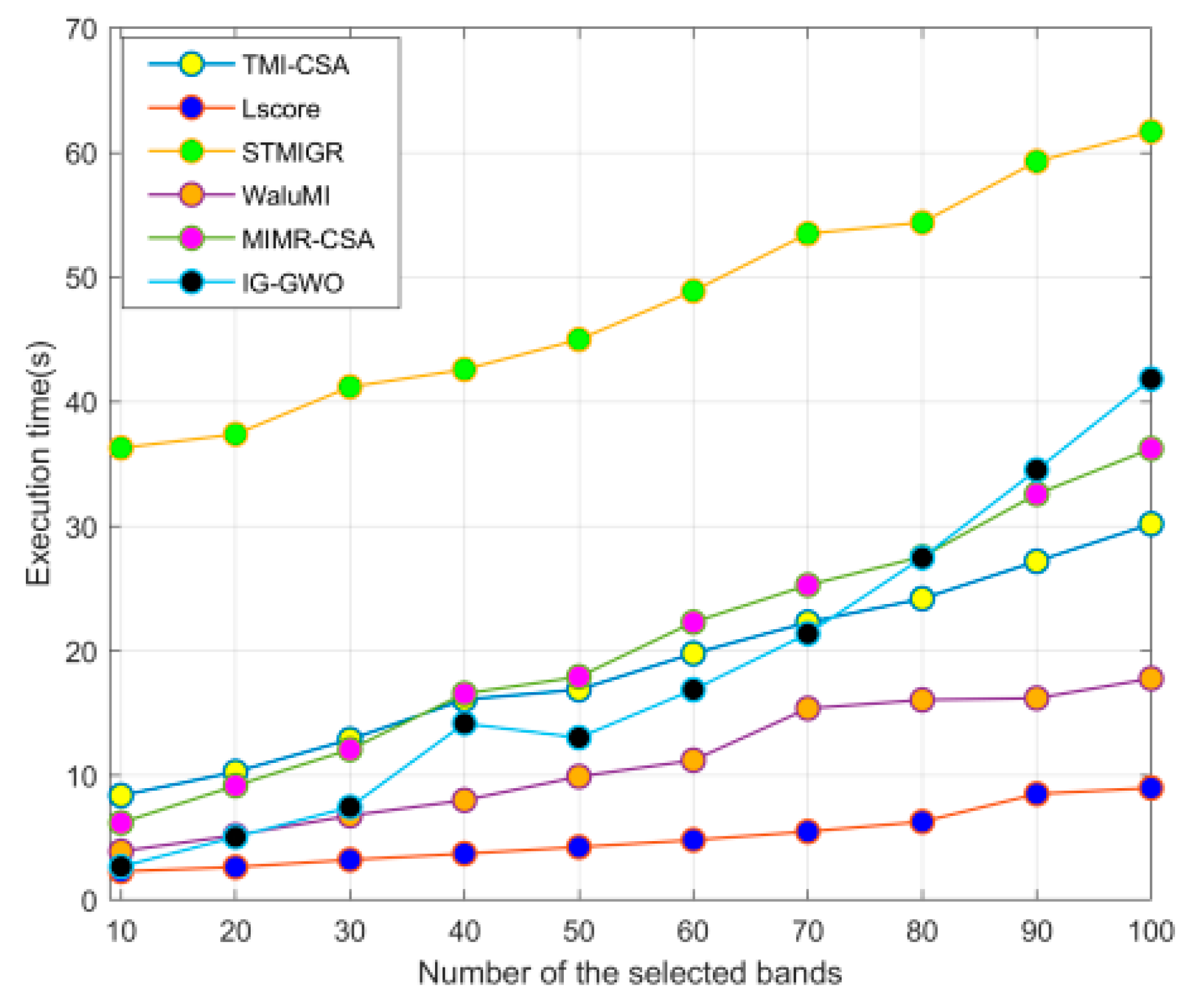
In this study, a novel hybrid filter-wrapper band selection method is introduced based on an improved subspace decomposition method and GWO optimization algorithm, and it is implemented through a three-step strategy: decomposition, selection and optimization. Extensive experimental results over the three hyperspectral datasets presented here clearly prove the effectiveness of the proposed method (IG-GWO), offering a solution to the aforementioned limitations and excelling compared to the other state-of-the-art band selection methods.

2. Materials and Methods

2.1. Information Gain (IG)

In machine learning and information theory, IG is a synonym for Kullback—Leibler divergence, which was introduced by Kullback and Leibler [47]. As a feature selection technique, IG has been widely applied to select a slice of important features for text classification. The larger the IG of a feature is, the more information it contains [48]. The computation of IG is based on entropy and conditional entropy.

Given a hyperspectral dataset $HD=\left\{x_1,x_2,\cdots ,x_n\right\}$ with l bands $\left\{B_1, B_2, \cdots ,B_l\right\}$ and q classes {C₁, C₂, …, C_q}, the IG of band B_i can be mathematically defined as below:

$$IG\left(C,Bi\right)=E\left(C\right)-E\left(C|B_i\right)$$

(1)

where E(C) denotes the entropy of dataset HD, and E(C|B) is the conditional entropy. E(C) and E(C|B_i) are expressed as follows:

$$E\left(C\right)=-{{\displaystyle \sum }}_{j=1}^{q}p\left(C_j\right)\log p\left(C_j\right)=-{{\displaystyle \sum }}_{j=1}^q\frac{N_{Bm}^j}{N_{Bm}}\log \frac{N_{Bm}^j}{N_{Bm}}$$

(2)

$$E\left(C|B_i\right)=-{{\displaystyle \sum }}_{m=1}^k\frac{N_{Bm}}{\left|\mathrm{HD}\right|}\left({{\displaystyle \sum }}_{j=1}^q\frac{N_{Bm}^j}{N_{Bm}}\log \frac{N_{Bm}^j}{N_{Bm}}\right)$$

(3)

where $|·|$ denotes the cardinality of the set, and N_Bm indicates the number of pixels in the m-th set that was obtained by using the band B_i to partition the hyperspectral dataset into k different sets via their intensity value G. Assuming a hyperspectral image with a radiometric resolution of 8 bits, the intensity value G of pixels in the image will have 256 gray levels; $N_{Bm}^j$ is the number of pixels belonging to the j-th class in the m-th set.

The band with the highest IG value is characterized by better classification performance. However, it is possible that the bands with high IG values will concentrate on a band subinterval. In this case, a flawed classification result will be obtained because the adjacent bands generally have a strong correlation. In addition, we do not know how to properly pre-assign the threshold to select them. Consequently, it is difficult to directly select such bands from the original bands to reduce the dimension of the hyperspectral dataset by using IG values only.

2.2. Gray Wolf Optimizer (GWO)

Very recently, a more powerful optimization method, the gray wolf optimizer, was proposed by Mirjalili [30]. This algorithm simulated the living and hunting behavior of a group of gray wolves. All gray wolves were divided hierarchically into four groups, denoted in turn as alpha wolf, beta wolf, delta wolf and omega wolf. In the first group, there was only a gray wolf, the alpha wolf, which was the leader of the others and controlled the whole wolf pack. The beta wolf only obeyed the alpha wolf in the second group and helped the alpha wolf to make some decisions and commanded the rest of the wolves in the two lower levels. The alpha wolf would be replaced by the beta wolf if the alpha wolf passed away. The gray wolves in the fourth group were named omega wolves and were responsible for collecting useful information to submit to the alpha wolf and beta wolf. The remainders were called delta wolves. The hunting procedure of gray wolves was carried out in three steps: tracking, pursuing and attacking the prey.

The social hierarchy and hunting procedure can be mathematically described as follows:

$\alpha$: The fittest solution;

$\beta$: The second-best solution;

$\delta$: The third-best solution;

$\omega$: The remaining candidate solutions.

The mathematical model of encircling the prey can be described as

$$\stackrel{\rightharpoonup }{D}=\left|\stackrel{\rightharpoonup }{C}·\stackrel{\rightharpoonup }{X_p}\left(t\right)-\stackrel{\rightharpoonup }{X}\left(t\right)\right|$$

(4)

$$\stackrel{\rightharpoonup }{X}\left(t+1\right)=\stackrel{\rightharpoonup }{X_p}\left(t\right)-\stackrel{\rightharpoonup }{A}·\stackrel{\rightharpoonup }{D}$$

(5)

where t denotes the current iteration;$\stackrel{\rightharpoonup }{D}$ represents the distance between the gray wolf and the prey; $\stackrel{\rightharpoonup }{A}$ and $\stackrel{\rightharpoonup }{C}$ are coefficient vectors; $\stackrel{\rightharpoonup }{ X_p}$ is the position vector of the prey and $\stackrel{\rightharpoonup }{X}$ the position vector of a gray wolf. The symbol. represents the corresponding multiplication of each component of two vectors.

The coefficient vectors A and C can be obtained by

$$\stackrel{\rightharpoonup }{A}=2\stackrel{\rightharpoonup }{a}·\stackrel{\rightharpoonup }{r_1}-\stackrel{\rightharpoonup }{a}$$

(6)

$$\stackrel{\rightharpoonup }{C}=2·\stackrel{\rightharpoonup }{r_2}$$

(7)

where components of $\stackrel{\rightharpoonup }{a}$ linearly decrease from 2 to 0 over the course of iterations; $\stackrel{\rightharpoonup }{r_1}$ and $\stackrel{\rightharpoonup }{r_2}$ are random vectors.

The mathematical model of hunting is

$$\stackrel{\rightharpoonup }{D_{\alpha }}=\left|\stackrel{\rightharpoonup }{C_1}·\stackrel{\rightharpoonup }{X_{\alpha }}\left(t\right)-\stackrel{\rightharpoonup }{X}\right|,\stackrel{\rightharpoonup }{ D_{\beta }}=\left|\stackrel{\rightharpoonup }{C_2}·\stackrel{\rightharpoonup }{X_{\beta }}\left(t\right)-\stackrel{\rightharpoonup }{X}\right|, \stackrel{\rightharpoonup }{D_{\delta }}=\left|\stackrel{\rightharpoonup }{C_3}·\stackrel{\rightharpoonup }{X_{\delta }}\left(t\right)-\stackrel{\rightharpoonup }{X}\right|$$

(8)

$$\stackrel{\rightharpoonup }{X_1}=\stackrel{\rightharpoonup }{X_{\alpha }}-\stackrel{\rightharpoonup }{A_1}·\stackrel{\rightharpoonup }{D_{\alpha }},\stackrel{\rightharpoonup }{X_2}=\stackrel{\rightharpoonup }{X_{\beta }}-\stackrel{\rightharpoonup }{A_2}·\stackrel{\rightharpoonup }{D_{\beta }},\stackrel{\rightharpoonup }{X_3}=\stackrel{\rightharpoonup }{X_{\delta }}-\stackrel{\rightharpoonup }{A_3}·\stackrel{\rightharpoonup }{D_{\delta }}$$

(9)

$$\stackrel{\rightharpoonup }{X}\left(t+1\right)=\stackrel{\rightharpoonup }{(X_1}+\stackrel{\rightharpoonup }{X_2}+\stackrel{\rightharpoonup }{X_3})/3$$

(10)

Repeating Equations (4)–(10), one can eventually compute the best solution $\stackrel{\rightharpoonup }{X_{\alpha }}$.

It should be noted that this theory is valid in a continuous case. If we slightly revise Equation (10) by rounding the operation, this algorithm can be used in a discrete case.

The GWO algorithm is summarized by the following steps:

Step 1

Initialize the gray wolf population GW_i (= 1, 2, …, N); parameters $\stackrel{\rightharpoonup }{a}$; maximum iterations;

Step 2

Select the alpha, beta and delta wolves from the population by calculating fitness;

Step 3

Update the position of each wolf by Equation (10);

Step 4

Compute Equations (4)–(9) and go to step 2;

Step 5

Output alpha until the iterations reach their maximum or the choice of the same alpha wolf twice in succession is satisfied.

To select the most distinguished band combination for increasing classification accuracy, it is important to choose/define the fitness function in step 2. The information gain (IG) is adopted as the fitness function in this study. Unlike the adoption of overall accuracy (OA) as fitness, one of the advantages of adopting IG as fitness is to effectively reduce the computation time of the GWO method since the computation of IG has nothing to do with the classification results.

Provided that there are s bands in a band combination (gray wolf), the IG value can be computed by Equation (11):

$${{\displaystyle \sum }}_{i=1}^{s}IG\left(C,B_i\right).$$

(11)

where $IG\left(C,B_i\right)$ is the information gain value of i-th band obtained from Equations (1)–(3).

2.3. The Proposed Band Selection Method

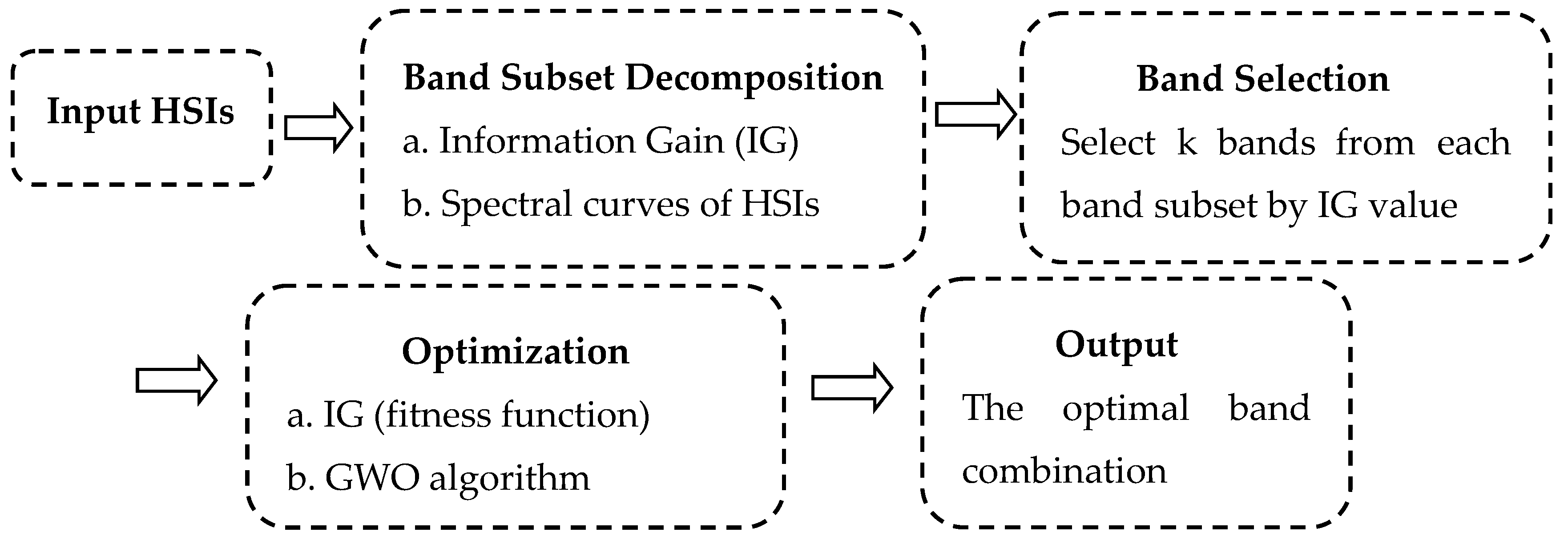
In this study, we integrate band subset decomposition, band selection and a GWO optimization algorithm to select the optimal band combination. The framework of the proposal is described in Figure 1.

Band subset decomposition is the partitioning of the original bands into different subsets so that bands in the same subset are similar to each other, and bands from different subsets are dissimilar. With this process, bands in different subsets enjoy different classification performances. Obviously, it is arduous to actualize band subset decomposition by only using the IG value. Therefore, in this work, we introduce an improved subset decomposition technique by simultaneously considering the spectral curve of the hyperspectral dataset and local minimal value method.

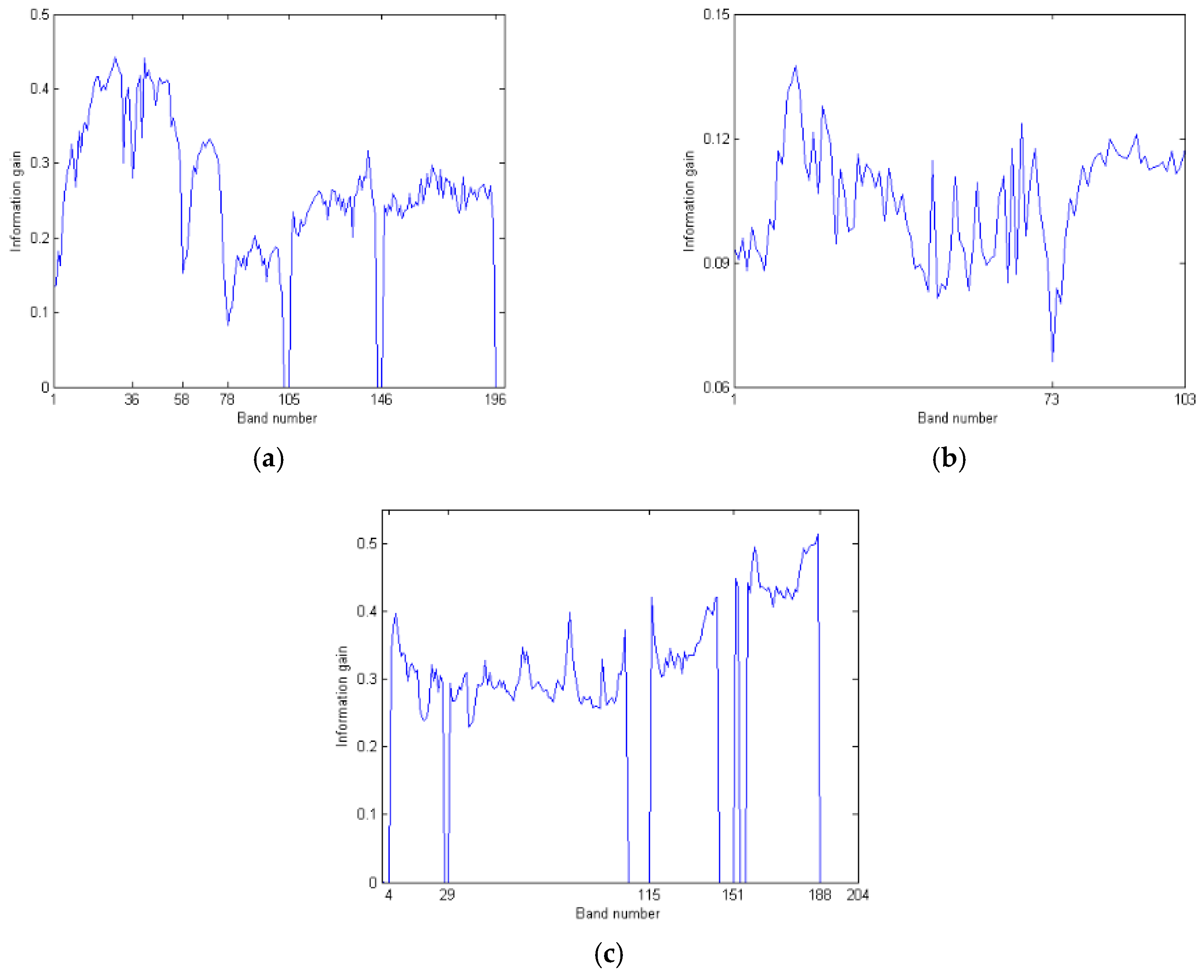
Specifically, for a given HSI, the information gain of each band is first calculated by Equations (1)–(3). The number c of band subsets is determined by the line chart of information gain in the spectral curve of the HSI. Finally, one can properly partition all bands into c different band subsets.

Regarding band selection, the spectral curve of the hyperspectral data set implies that the spectral curves of each pixel in a certain interval are similar in shape and only different from each other in radiance. This means that bands that are located in the same interval have a similar distinguishing capacity for different land surface features. Consequently, it is logical to replace all bands in the same subset with several selected bands in an attempt to maintain similar classification results. This process implies that some of the redundant bands are abandoned.

On the basis of c different subsets, one can obviously select the bands with high IG values from each subset. However, this may lead to the loss of substantial information. Alternately, we randomly select k different bands from each band subset to constitute a band combination in a process that is also known as gray wolf, ($b_{11},\dots ,b_{1k},\dots \dots , b_{c1},\dots ,b_{ck}$). The component $b_{ij}$ in gray wolf denotes the selected j-th band from i-th subset. This ensures that each band subset has the same contribution to the classification result. It is notable that the acquired band combination has less band redundancy, but this does not mean that it has good classification performance. Thus, the GWO algorithm is employed to optimize it to provide a satisfactory classification performance. The GWO algorithm is chosen as the optimization method because the GWO algorithm shows very good performance in exploration, local minima avoidance, and exploitation, simultaneously [30].

Regarding optimization: suppose that there are N gray wolves in the initial population. The IG value of each gray wolf in the initial population is computed by using Equations (1)–(3) and (11). One then performs a descending sort of the IG values, with the largest in front. The wolves that correspond to the three largest IG values are called the alpha wolf, beta wolf and delta wolf, one after the other. The rest are designated as omega wolves. In the absence of information about the location of the prey, the position vector of the prey is replaced approximately by the position of the alpha wolf. The following supposes that each of the gray wolves knows the location of prey and encircles it [30,33].

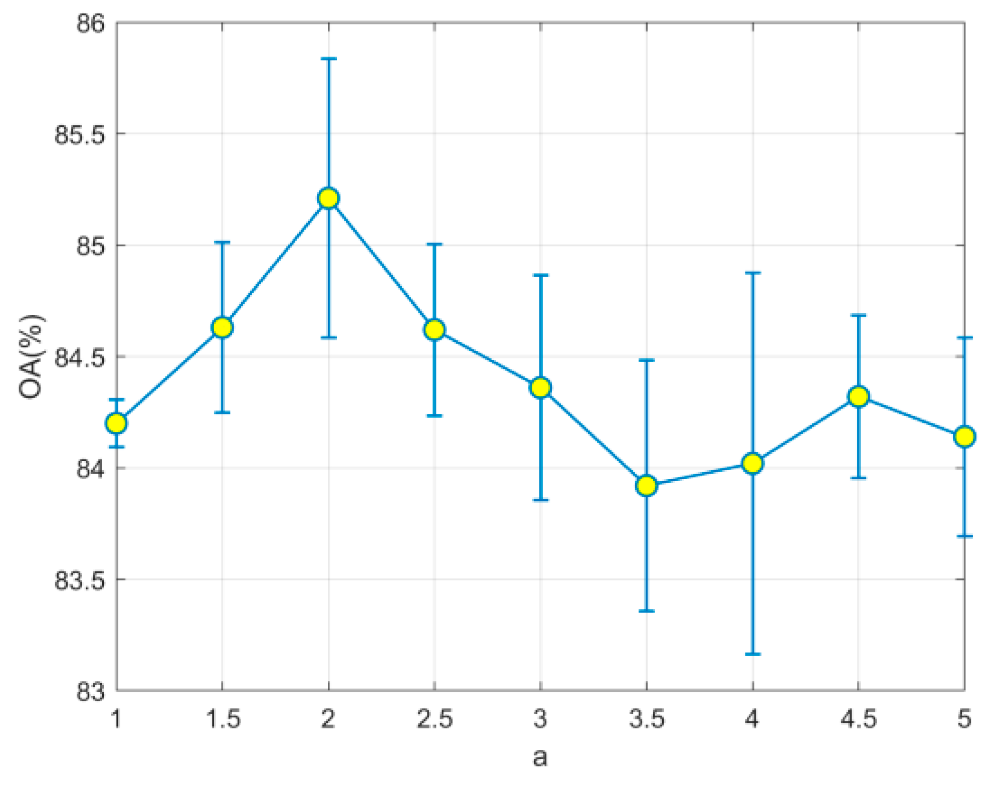
Encircling the prey during the hunt can be performed by Equations (4)–(7) and setting a = 2.

After encircling the prey, each wolf should quickly update its position relative to the locations of the alpha, beta and delta wolves in order to enclose the prey. The hunting process is accomplished by computing Equations (8)–(10).

The proposed band selection algorithm IG-GWO can be summarized as follows:

Input: Hyperspectral dataset; parameters $\stackrel{\rightharpoonup }{a}$ and maximum iterations.

Output: The most informative feature, subset $\alpha$.

Step 1: Divide the initial bands into c subsets by their IG value and the spectral curve of the hyperspectral dataset.

Step 2: Randomly select k different bands from each subset to constitute a gray wolf.

Step 3: Initialize the population in GWO by repeatedly performing step 2 N times.

Step 4: Call the GWO algorithm mentioned in Section 2.2.

3. Results

3.1. Experimental Setup and Description of the Dataset

To assess the performance of the proposed method, three typical hyperspectral datasets, Indian Pines, Pavia University and Salinas [50], were chosen for our experiments. A support vector machine with five-fold cross-validation (SVM-5) is applied to classify the selected three datasets. Classification is actualized through the one-against-all approach, and the Gaussian radial basis function (RBF) kernel is adopted as its kernel function in SVM-5. The optimal parameters C and γ of the RBF kernel are determined via five-fold cross-validation. TMI-CSA (clonal selection algorithm) [45], Lscore [44], STMIGR [45], WaLuMI [20] and MIMR-CSA (clonal selection algorithm) [23] are used as the comparison methods. The reason for choosing these five algorithms is that the same classifiers, labeling proportions and precision evaluation indicators are used in these five algorithms with the suggested methods.

In all experiments, 5%, 10%, 15% and 20% of instances in each class are randomly labeled to compose the training sets. The rest are to be classified directly. In order to reduce the influence of random labeling on the classification result, all experiments are conducted over 30 independent runs with a random choice of training set. The average value and standard deviation of classification accuracy are reported in the following tables. The initial population in the GWO algorithm consists of N = 30 gray wolves. The maximum number of iterations is set to 50 in the GWO algorithm.

To quantitatively appraise the classification result of the hyperspectral dataset, the three universal indices [51] of overall accuracy (OA), average accuracy (AA), and kappa coefficient (KC) are adopted in this study.

(1)

Overall accuracy (OA) refers to the number of correctly classified instances divided by the total number of testing samples;

(2)

Average accuracy (AA) is a measure of the mean value of the classification accuracies of all classes;

(3)

The kappa coefficient (KC) is a statistical measurement of consistency between the ground truth map and the final classification map.

The Indian pines image [50] was collected by the Airborne Visible Infrared Imaging Spectrometer (AVIRIS) sensor at the Indian pine test station located in northwestern Indiana in 1992. It contains 145 × 145 pixels and 200 available spectral reflectance bands (eliminating the 20 water absorption bands) in the wavelength range from 0.4 to 2.5 μm. The spatial resolution is 20 m/pixel. The 16 classes of vegetation and forests are contained in the image, as well as the specific types of ground objects that can be found in the legend (Figure 2). A three-feature false-color composite image and its ground truth image are displayed in Figure 2a,b, respectively.

The Pavia University image was captured by the Reflective Optics System Imaging Spectrometer (ROSIS) sensor over Pavia, Northern Italy [50]. Each band image comprises 610 × 340 samples with a spatial resolution of 1.3 m/pixel. In each band scene, there are nine classes of representative urban ground objects. After removing 12 noisy spectral bands, 103 usable bands are retained for the following research. A three-feature false-color composite image and ground truth image are separately exhibited (Figure 3a,b).

The Salinas scene was also gathered by the AVIRIS sensor over Salinas Valley, California (Figure 3). The image has a spatial dimension of 512 × 217 pixels and a spatial resolution of 3.7 m/pixel. The AVIRIS sensor generates 224 spectral bands (eliminating 20 water absorption bands), and 204 bands remain for the subsequent experiment. The Salinas image consists of 16 classes of ground objects, covering vegetables, fields, bare soils, and so on [50]. A three-feature false-color composite image and its ground truth image are shown (Figure 4a,b).

Some of the main features of the three datasets are summarized in

Table 1. The description of three hyperspectral datasets. ROSIS: Reflective Optics System Imaging Spectrometer.

Class Number	Indian Pines	Pavia University	Salinas
	16	9	16
Bands	200	103	204
Size	$145\times 145$	$610\times 340$	$512\times 217$
Sensor	AVIRIS	ROSIS	AVIRIS
Resolution	20 m	1.3 m	3.7 m
Samples	10,249	42,776	54,129

.

3.2. Classification Results.

Based on the information gain and spectral curve of three hyperspectral datasets (Figure 5), one can properly decompose the Indian Pines dataset into six band subsets, which are (1~36), (37~58), (59~78), (79~105), (106~146) and (147~200). The Pavia University dataset can be divided into two band subsets, which are (1~73) and (74~103). The Salinas dataset may be separated into four band subsets, which are (1~29), (30~115), (116~151) and (152~204). Based on a specific dataset and its band subset decomposition, k different bands in each subset are randomly selected to consist of a gray wolf (k = 1, 2, ..., 7 for the Indian Pines and Salinas datasets and k = 3, 6, 9, 12, 15, 18 for the Pavia University dataset). Then, the most informative band subset is outputted by applying the proposed IG-GWO algorithm.

In the second lines in

Table 2. The classification results over overall accuracy (OA), average accuracy (AA) and kappa coefficient (KC) (%) on the Indian Pines dataset (the numbers marked in bold represent the best classification results).

Label Ratio Index		Number of the Selected Bands
		6	12	18	24	30	36	42
5%	OA	72.56 ± 1.7	75.24 ± 1.6	75.18 ± 3.1	75.36 ± 2.9	76.19 ± 1.9	76.15 ± 1.5	77.09 ± 1.3
	AA	63.10 ± 13.9	64.97 ± 11.6	65.32 ± 14.9	67.07 ± 16.8	67.03 ± 13.7	64.73 ± 13.7	65.79 ± 10.9
	KC	68.43 ± 2.2	71.54 ± 1.8	71.53 ± 3.7	71.71 ± 3.4	72.67 ± 2.2	72.67 ± 1.8	73.72 ± 1.5
10%	OA	76.96 ± 0.9	79.72 ± 1.9	80.61 ± 1.7	80.39 ± 1.9	81.07 ± 1.1	81.35 ± 1.2	82.29 ± 1.5
	AA	72.55 ± 11.9	73.08 ± 9.2	73.95 ± 14.5	74.38 ± 12.5	75.26 ± 8.5	73.34 ± 10.2	75.10 ± 9.6
	KC	73.58 ± 1.1	76.79 ± 2.2	77.81 ± 2.0	77.55 ± 2.4	78.32 ± 1.2	78.67 ± 1.4	79.74 ± 1.8
15%	OA	78.64 ± 0.5	81.87 ± 1.2	82.86 ± 1.0	82.68 ± 1.2	83.59 ± 0.7	83.68 ± 0.7	84.61 ± 0.4
	AA	76.93 ± 8.9	78.45 ± 8.4	79.20 ± 7.0	79.44 ± 7.8	80.34 ± 7.3	79.72 ± 6.6	79.98 ± 10.8
	KC	75.52 ± 0.5	79.26 ± 1.4	80.41 ± 1.2	80.17 ± 1.4	81.25 ± 0.8	81.34 ± 0.9	82.41 ± 0.5
20%	OA	79.49 ± 0.5	83.75 ± 0.6	83.98 ± 1.1	84.40 ± 1.3	85.21 ± 0.8	85.12 ± 0.6	86.15 ± 0.7
	AA	77.80 ± 7.4	81.53 ± 6.9	81.02 ± 7.0	81.55 ± 6.8	82.59 ± 6.6	80.89 ± 6.7	83.69 ± 9.4
	KC	76.51 ± 0.5	81.43 ± 0.8	81.70 ± 1.3	82.16 ± 1.5	83.10 ± 0.9	82.99 ± 0.7	84.18 ± 0.8

,

Table 3. The classification results over OA, AA and KC (%) on the Pavia University dataset (the numbers marked in bold represent the best classification results).

Label Ratio Index		Number of the Selected Bands
		6	12	18	24	30	36
5%	OA	88.25 ± 0.5	90.62 ± 0.4	92.26 ± 0.5	92.89 ± 0.3	92.86 ± 0.5	93.00 ± 0.5
	AA	84.34 ± 2.8	87.87 ± 2.3	89.61 ± 2.4	90.61 ± 2.4	90.58 ± 2.1	90.54 ± 1.9
	KC	84.19 ± 0.8	87.44 ± 0.6	89.68 ± 0.7	90.53 ± 0.5	90.48 ± 0.7	90.66 ± 0.7
10%	OA	89.08 ± 0.2	91.62 ± 0.2	93.35 ± 0.5	93.82 ± 0.3	93.67 ± 0.2	94.11 ± 0.3
	AA	85.72 ± 1.8	89.35 ± 1.4	91.16 ± 1.4	91.73 ± 1.6	91.52 ± 1.6	92.04 ± 1.5
	KC	85.35 ± 0.2	88.80 ± 0.3	91.15 ± 0.7	91.77 ± 0.4	91.57 ± 0.3	92.16 ± 0.4
15%	OA	89.46 ± 0.2	92.02 ± 0.2	93.80 ± 0.1	94.32 ± 0.3	94.29 ± 0.2	94.66 ± 0.2
	AA	86.39 ± 1.7	89.92 ± 1.2	91.76 ± 1.6	92.33 ± 1.2	92.23 ± 0.9	92.71 ± 1.1
	KC	85.87 ± 0.3	89.35 ± 0.2	91.75 ± 0.2	92.45 ± 0.3	92.41 ± 0.3	92.89 ± 0.2
20%	OA	89.73 ± 0.2	92.40 ± 0.2	94.21 ± 0.2	94.67 ± 0.2	94.51 ± 0.1	94.88 ± 0.2
	AA	86.60 ± 1.6	90.29 ± 1.3	92.25 ± 1.0	92.76 ± 0.9	92.50 ± 1.0	92.99 ± 1.4
	KC	86.23 ± 0.3	89.85 ± 0.2	92.30 ± 0.2	92.92 ± 0.2	92.70 ± 0.1	93.20 ± 0.2

and

Table 4. The classification results over OA, AA and KC (%) on the Salinas dataset (the numbers marked in bold represent the best classification results).

Label Ratio Index		Number of the Selected Bands
		4	8	12	16	20	24	28
5%	OA	89.34 ± 0.4	91.37 ± 0.3	91.71 ± 0.5	91.86 ± 0.6	91.92 ± 0.3	92.45 ± 0.4	92.34 ± 0.3
	AA	93.28 ± 1.9	94.86 ± 1.5	95.24 ± 1.4	95.46 ± 1.4	95.52 ± 1.2	95.76 ± 1.7	95.66 ± 1.7
	KC	88.09 ± 0.4	90.37 ± 0.3	90.75 ± 0.6	90.92 ± 0.7	90.99 ± 0.3	91.58 ± 0.5	91.46 ± 0.3
10%	OA	89.87 ± 0.2	91.90 ± 0.2	92.40 ± 0.3	92.69 ± 0.2	92.64 ± 0.2	93.20 ± 0.3	93.07 ± 0.3
	AA	94.03 ± 1.2	95.44 ± 1.2	95.93 ± 0.8	96.19 ± 1.0	96.15 ± 0.9	96.41 ± 1.0	96.36 ± 0.9
	KC	88.69 ± 0.2	90.96 ± 0.3	91.52 ± 0.4	91.85 ± 0.3	91.79 ± 0.3	92.42 ± 0.3	92.28 ± 0.4
15%	OA	90.01 ± 0.3	92.22 ± 0.2	92.75 ± 0.3	93.15 ± 0.2	93.03 ± 0.3	93.67 ± 0.2	93.53 ± 0.2
	AA	94.23 ± 1.0	95.79 ± 0.7	96.29 ± 0.9	96.62 ± 0.7	96.50 ± 0.8	96.80 ± 0.7	96.80 ± 0.7
	KC	88.84 ± 0.3	91.32 ± 0.3	91.91 ± 0.3	92.36 ± 0.3	92.22 ± 0.3	92.95 ± 0.2	92.79 ± 0.3
20%	OA	90.15 ± 0.1	92.36 ± 0.2	93.01 ± 0.1	93.30 ± 0.1	93.29 ± 0.2	93.91 ± 0.2	93.89 ± 0.2
	AA	94.40 ± 0.8	95.92 ± 0.5	96.49 ± 0.6	96.72 ± 0.5	96.68 ± 0.6	96.98 ± 0.6	97.03 ± 0.7
	KC	89.01 ± 0.1	91.47 ± 0.2	92.21 ± 0.1	92.52 ± 0.1	92.52 ± 0.2	93.22 ± 0.2	93.19 ± 0.2

, the number of the optimal bands is the product of the number k and the number of band subsets. The numbers in the first columns in Table 2, Table 3 and Table 4 are sampling ratios.

The classification results of the Indian Pines dataset that were obtained by the proposed method are reported in Table 2. The best classification by OA achieves an accuracy of 86.15% ± 0.7% (42 optimized bands and a labeling ratio of 20%). The classification results over OA and KC become increasingly better as the number of the selected bands increases. When the number of the selected bands ranges from 12 to 42, the three indices all exhibit a slow increase (approximately 2.5%) and no notable increase. This may be because the redundancy among the bands is increased as the number of selected bands increases. The classification results are unfavorable when six bands are selected because too much band information is lost.

The satisfactory classification results on the Pavia University dataset are listed in Table 3. The classification accuracy over OA (94.88% ± 0.2%) indicates that the pixels in this dataset are almost correctly classified by the proposed method. This means that more informative bands can be selected by the proposed IG-GWO algorithm. Three indices have little variety and represent a stable tendency as the number of the selected bands increases from 18 to 36.

The classification results on the Salinas dataset are shown in Table 4. From the top-left to the lower right in Table 4, the three indices all present a growing trend. This pattern occurs because the classification accuracy increases as the number of selected bands and the sampling proportion increase. However, it is clear that there is a small difference in the classification results between 20 bands and 28 bands. This result again confirms that the distinctive bands can be selected from the original bands by our proposal. This better result proves the effectiveness of the proposed method.

3.3. Comparative Analysis of Classification Results

To fairly compare our proposal with the other five band selection methods, the same random sampling proportion of 20% and classifiers are taken for the comparison experiments. In the other five approaches, the number of the selected bands is 30 for the Indian Pines and Salinas datasets and 20 for the Pavia University dataset. Based on the band subset decomposition and band selection strategy, the exact band number could not be obtained in our proposal. Accordingly, band number 18 for the Pavia University dataset and band number 28 for the Salinas dataset are adopted and are close to those of the other five methods. The comparison results of the six algorithms for the three datasets are listed in

Table 5. The comparison results of six algorithms on the Indian Pines dataset. STMIGR: semi-supervised band selection approach based on TMI and graph regulation; WaLuMI: Ward’s linkage and MI method; IG-GWO: information gain–grey wolf optimization.

Method	OA (%)	AA (%)	KC (%)
TMI-CSA	72.9 ± 2.0	55.5 ± 2.3	68.7 ± 2.3
Lscore	73.9 ± 0.5	61.4 ± 1.1	70.0 ± 0.6
STMIGR	74.4 ± 1.0	57.4 ± 1.2	70.4 ± 1.2
WaLuMI	80.6 ± 0.8	68.2 ± 2.0	77.7 ± 1.0
MIMR-CSA	84.5 ± 0.9	79.4 ± 1.8	82.3 ± 1.0
IG-GWO	85.2 ± 0.8	82.6 ± 6.6	83.1 ± 0.9

,

Table 6. The comparison results of six algorithms on the Pavia University dataset.

Method	OA (%)	AA (%)	KC (%)
TMI-CSA	86.2 ± 1.6	79.4 ± 2.7	81.4 ± 2.2
Lscore	87.5 ± 1.7	82.6 ± 2.7	83.2 ± 2.3
STMIGR	87.2 ± 1.5	82.8 ± 1.6	82.8 ± 2.0
WaLuMI	90.1 ± 1.0	86.7 ± 1.2	86.7 ± 1.4
MIMR-CSA	92.5 ± 0.3	89.1 ± 0.6	90.1 ± 0.3
IG-GWO (18 bands)	94.2 ± 0.2	92.3 ± 1.0	92.3 ± 0.2

and

Table 7. The comparison results of six algorithms on the Salinas dataset.

Method	OA (%)	AA (%)	KC (%)
TMI-CSA	90.8 ± 0.2	94.3 ± 0.2	89.8 ± 0.2
Lscore	91.7 ± 0.6	95.7 ± 0.3	90.7 ± 0.6
STMIGR	91.3 ± 0.3	95.3 ± 0.3	90.3 ± 0.3
WaLuMI	93.0 ± 0.2	96.4 ± 0.2	92.2 ± 0.2
MIMR-CSA	93.5 ± 0.2	96.8 ± 0.1	92.7 ± 0.2
IG-GWO (28 bands)	93.9 ± 0.2	97.0 ± 0.7	93.2 ± 0.2

.

One can easily see from Table 5, Table 6 and Table 7 that the proposal outperforms the other five algorithms on the three datasets. The positive classification results have not been obtained by the six algorithms on the Indian Pines dataset, partially due to the complexity of the ground-truth. However, better classification results have been achieved on the Salinas dataset by these six methods since all of the classification accuracies over OA and AA are greater than 90%. The MIMR-CSA method is more competitive than the other four methods. As shown in Table 5 and Table 7, the classification results on the Indian Pines and Salinas datasets show few differences between the MIMR-CSA method and our proposal. In addition, the TMI-CSA, Lscore, and STMIGR methods cannot effectively classify the Indian Pines and Pavia University datasets, as shown in Table 5 and Table 6. It should be noted that excellent results can still be obtained by the proposed method in the absence of two bands in the Pavia University and Salinas datasets.

The classification results of each class on the three datasets are presented in Figure 6. For most classes, the classification accuracies that are obtained by our proposal are greater than or equal to those that are provided by the other five algorithms. Figure 6c clearly explains why the values of index AA are greater than those of OA on the Salinas dataset since 14 out of 16 classes are almost correctly classified. The TMI-CSA and STMIGR methods result in dreadful classification results, such as the 7th class (grass/pasture-mowed) and 9th class (Oats) in the Indian Pines dataset and the 3rd class (gravel) and 7th class (bitumen) in the Pavia University dataset.

In Medjahed et al. [33], the authors directly applied the GWO algorithm to select optimal candidate bands by defining five objective functions by their fitness. Based on the selected bands, they used a K nearest neighbor (KNN) classifier to perform classification. The best classification result (OA) that they provided was 73.67% on Indian Pines, 88.17% on Pavia University and 95.38% on Salinas. We here have not compared our results with theirs in Table 5, Table 6 and Table 7 since different classifiers are used. Furthermore, the authors did not clearly point out how many bands were selected for their final classification results. Regarding Table 2, Table 3 and Table 4 and in the case of the same sampling of 10% of the pixels, the superiority of the proposed method is obvious.

3.4. Sensitivity and Computing Time Analysis

In what follows, for simplicity, we will take the Indian Pines dataset as an example in order to analyze the variation of the average classification accuracies obtained by the six algorithms as the number of selected features increases from 10 to 100. It can be seen in Figure 7 that our algorithm achieves better classification results when the number of the selected bands is less than or equal to 40. This indicates that the most informative bands can be found by the proposed method. The classification accuracies of the six algorithms all show an upward trend as the number of selected bands increases. However, due to the sharp increase in redundancy between bands, the classification accuracy does not show a notable increase as the number of selected bands multiplies.

Figure 8 records the computing time of the six approaches for the Indian Pines dataset. Among the six algorithms, Lscore takes the least amount of time due to the ranking-based search that is without iteration. Compared to the other five algorithms, STMIGR is very time-consuming since the construction of the adjacent graph by the samples is necessary. With the exception of the STMIGR algorithm, all of the other five algorithms show good time implementation. Combined with Figure 7 and Figure 8, we can see that the IG-GWO and MIMR-CSA algorithms show good classification abilities and implementation.

When OA and IG are adopted as fitness functions in the optimization process, Figure 9 shows the classification results that are obtained by using the IG-GWO method and single GWO algorithm. Based on these two fitness functions, the proposed method acquires a better classification accuracy. The classification difference between the two fitness functions is less than 2%. Starting from the selection of the bands with high IG values, the GWO algorithm using both OA and IG as fitness is directly applied to search for the optimal band combination. As a result, their classification results are lower than those obtained by the IG-GWO method. The GWO algorithm using OA as fitness shows instability, which may be because the optimization algorithm is terminated before the optimal band combination is found. After all, for a data set with 200 bands, there are too many band combinations. GWO with IG as fitness provides poor classification results because there is much redundancy in the resulting band combinations, which leads to the decline of classification ability. This fully illustrates the necessity of carrying out subset decomposition in the proposed method.

As shown in Figure 10, the computing time of the algorithm adopting IG as the fitness function is much less than that with OA. Theoretically, if OA is used as the fitness function, the GWO algorithm needs to implement the classification algorithm (SVM) in each iteration, which undoubtedly increases the computation time of the algorithm. This result is consistent with the theoretical analysis.

It is necessary to analyze the effect of parameter changes on classification accuracy. In the proposal, parameter a controls the optimization range and the convergence rate of the GWO algorithm. A small a value means that the optimization range of GWO is smaller and the convergence speed is faster. Figure 11 records the variability classification accuracies with different parameters for a. There is approximately a 1% difference between the maximum classification accuracy and the minimum classification accuracy. This shows, to a certain extent, that the algorithm proposed in this paper is relatively stable.

4. Conclusions

In this work, a novel hybrid filter-wrapper band selection method is introduced by a three-step strategy that is based on the improved band subset decomposition method and the GWO optimization algorithm. For the selected band combination, the first two steps attempt to reduce the redundancy between the spectral bands, and the last step ensures that the combination has a good classification performance. The proposed method inherits the advantages of a high classification accuracy based on the wrapper method and a fast computing speed based on the filter algorithm. The experimental results reveal that this attempt achieves a reasonable compromise between computing time and classification accuracy. The comparative experimental results on three typical hyperspectral datasets successfully confirm that the proposal is more powerful than several existing approaches.

References

1. Cao, X.; Wei, C.; Han, J.; Jiao, L. Hyperspectral Band Selection Using Improved Classification Map. IEEE Geosci. Remote Sens. Lett. 2017, 14, 2147–2151. [Google Scholar] [CrossRef]
2. Zhang, M.; Ma, J.; Gong, M. Unsupervised Hyperspectral Band Selection by Fuzzy Clustering with Particle Swarm Optimization. IEEE Geosci. Remote Sens. Lett. 2017, 14, 773–777. [Google Scholar] [CrossRef]
3. Khanal, S.; Fulton, J.; Shearer, S. An overview of current and potential applications of thermal remote sensing in precision agriculture. Comput. Electron. Agric. 2017, 139, 22–32. [Google Scholar] [CrossRef]
4. Nielsen, M. Remote sensing for urban planning and management: The use of window-independent context segmentation to extract urban features in Stockholm. Comput. Environ. Urban Syst. 2015, 52, 1–9. [Google Scholar] [CrossRef]
5. Padmanaban, R.; Bhowmik, A.; Cabral, P. A Remote Sensing Approach to Environmental Monitoring in a Reclaimed Mine Area. ISPRS Int. J. Geo-Inf. 2017, 6, 401. [Google Scholar] [CrossRef]
6. Prasad, D.K.; Agarwal, K. Classification of Hyperspectral or Trichromatic Measurements of Ocean Color Data into Spectral Classes. Sensors 2016, 16, 3. [Google Scholar] [CrossRef] [PubMed]
7. Yang, J.; Jiang, Z.; Hao, S.; Zhang, H. Higher Order Support Vector Random Fields for Hyperspectral Image Classification. ISPRS Int. J. Geo-Inf. 2018, 7, 19. [Google Scholar] [CrossRef]
8. Ghamisi, P.; Benediktsson, J.A.; Ulfarsson, M.O. Spectral–Spatial Classification of Hyperspectral Images Based on Hidden Markov Random Fields. IEEE Trans. Geosci. Remote Sens. 2014, 52, 2565–2574. [Google Scholar] [CrossRef]
9. Patra, S.; Modi, P.; Bruzzone, L. Hyperspectral Band Selection Based on Rough Set. IEEE Trans. Geosci. Remote Sens. 2015, 53, 5495–5503. [Google Scholar] [CrossRef]
10. Zhang, J.; Wang, Y.; Zhao, W. An Improved Hybrid Method for Enhanced Road Feature Selection in Map Generalization. Int. J. Geo-Inf. 2017, 6, 196. [Google Scholar] [CrossRef]
11. Dong, Y.; Du, B.; Zhang, L.; Zhang, L. Dimensionality Reduction and Classification of Hyperspectral Images Using Ensemble Discriminative Local Metric Learning. IEEE Trans. Geosci. Remote Sens. 2017, 55, 2509–2524. [Google Scholar] [CrossRef]
12. Chang, C.; Du, Q.; Sun, T. A Joint Band Prioritization and Band-Decorrelation Approach to Band Selection for Hyperspectral Image Classification. IEEE Trans. Geosci. Remote Sens. 1999, 37, 2631–2641. [Google Scholar] [CrossRef]
13. Chang, C.; Su, W. Constrained Band Selection for Hyperspectral Imagery. IEEE Trans. Geosci. Remote Sens. 2006, 44, 1575–1585. [Google Scholar] [CrossRef]
14. Salas, E.A.L.; Henebry, G.M. A New Approach for the Analysis of Hyperspectral Data: Theory and Sensitivity Analysis of the Moment Distance Method. Remote Sens. 2013, 6, 20–41. [Google Scholar] [CrossRef] [Green Version]
15. Qian, Y.; Yao, F.; Jia, S. Band Selection for Hyperspectral Imagery Using Affinity Propagation. IET Comput. Vis. 2009, 3, 213–222. [Google Scholar] [CrossRef]
16. Wang, Q.; Yuan, Y.; Yan, P. Visual Saliency by Selective Contrast. IEEE Trans. Circuits Syst. Video Technol. 2013, 23, 1150–1155. [Google Scholar] [CrossRef]
17. Roweis, S.T.; Saul, L.K. Nonlinear Dimensionality Reduction by Locally Linear Embedding. Science 2000, 290, 2323. [Google Scholar] [CrossRef] [PubMed]
18. Agarwal, A.; El-Ghazawi, T.; El-Askary, H.; Le-Moigne, J. Efficient Hierarchical-PCA Dimension Reduction for Hyperspectral Imagery. In Proceedings of the IEEE International Symposium on Signal Processing and Information Technology, Giza, Egypt, 15–18 December 2008; pp. 353–356. [Google Scholar]
19. Li, W.; Prasad, S.; Fowler, J.E.; Bruce, L.M. Locality-Preserving Dimensionality Reduction and Classification for Hyperspectral Image Analysis. IEEE Trans. Geosci. Remote Sens. 2012, 50, 1185–1198. [Google Scholar] [CrossRef] [Green Version]
20. Martínez-Usómartinez-Uso, A.; Pla, F.; Sotoca, J.M.; García-Sevilla, P. Clustering-Based Hyperspectral Band Selection Using Information Measures. IEEE Trans. Geosci. Remote Sens. 2007, 45, 4158–4171. [Google Scholar] [CrossRef] [Green Version]
21. Guo, B.; Gunn, S.R.; Damper, R.I.; Nelson, J.D.B. Band Selection for Hyperspectral Image Classification Using Mutual Information. IEEE Geosci. Remote Sens. Lett. 2006, 3, 522–526. [Google Scholar] [CrossRef] [Green Version]
22. Talebi Nahr, S.; Pahlavani, P.; Hasanlou, M. Different Optimal Band Selection of Hyperspectral Images Using a Continuous Genetic Algorithm. In Proceedings of the ISPRS International Archives of the Photogrammetry, Remote Sensing and Spatial Information Sciences, Tehran, Iran, 15–17 November 2014; pp. 249–253. [Google Scholar]
23. Feng, J.; Jiao, L.; Liu, F.; Sun, T.; Zhang, X. Unsupervised feature selection based on maximum information and minimum redundancy for hyperspectral images. Pattern Recognit. 2016, 51, 295–309. [Google Scholar] [CrossRef]
24. Zheng, X.; Lu, X. Discovering Diverse Subset for Unsupervised Hyperspectral Band Selection. IEEE Trans. Image Process. 2017, 26, 51–64. [Google Scholar]
25. Zhong, N.; Dong, J.; Ohsuga, S. Using Rough Sets with Heuristics for Feature Selection. J. Intell. Inf. Syst. 2001, 16, 199–214. [Google Scholar] [CrossRef]
26. Lai, C.; Reinders, M.J.T.; Wessels, L. Random Subspace Method for Multivariate Feature Selection. Pattern Recognit. Lett. 2006, 27, 1067–1076. [Google Scholar] [CrossRef]
27. Mafarja, M.M.; Mirjalili, S. Whale Optimization Approaches for Wrapper Feature Selection. Appl. Soft Comput. 2017, 62, 441–453. [Google Scholar] [CrossRef]
28. Lehegarat-Mascle, S.; Vidal-Madjar, D.; Olivier, P. Applications of Simulated Annealing to SAR Image Clustering and Classification Problems. Int. J. Remote Sens. 2018, 17, 1761–1776. [Google Scholar] [CrossRef]
29. Ghamisi, P.; Benediktsson, J.A. Feature Selection Based on Hybridization of Genetic Algorithm and Particle Swarm Optimization. IEEE Geosci. Remote Sens. Lett. 2014, 12, 309–313. [Google Scholar] [CrossRef]
30. Mirjalili, S.; Mirjalili, S.M.; Lewis, A. Grey Wolf Optimizer. Adv. Eng. Softw. 2014, 69, 46–61. [Google Scholar] [CrossRef]
31. Karaboga, D.; Ozturk, C. A novel clustering approach: Artificial Bee Colony (ABC) algorithm. Appl. Soft Comput. 2011, 11, 652–657. [Google Scholar] [CrossRef]
32. Ghamisi, P.; Couceiro, M.S.; Martins, F.M.L.; Benediktsson, J.A. Multilevel Image Segmentation Based on Fractional-Order Darwinian Particle Swarm Optimization. IEEE Trans. Geosci. Remote Sens. 2014, 52, 2382–2394. [Google Scholar] [CrossRef] [Green Version]
33. Medjahed, S.; Saadi, T.; Benyettou, A.; Ouali, M. Gray Wolf Optimizer for hyperspectral band selection. Appl. Soft Comput. 2016, 40, 178–186. [Google Scholar] [CrossRef]
34. Khairuzzaman, A.K.M.; Chaudhury, S. Multilevel Thresholding Using Grey Wolf Optimizer for Image Segmentation. Expert Syst. Appl. 2017, 86, 64–76. [Google Scholar] [CrossRef]
35. Mirjalili, S.; Saremi, S.; Mirjalili, S.M.; Coelho, L.D.S. Multi-Objective Grey Wolf Optimizer: A Novel Algorithm for Multi-Criterion Optimization. Expert Syst. Appl. 2016, 47, 106–119. [Google Scholar] [CrossRef]
36. Rodríguez, L.; Castillo, O.; Soria, J.; Melin, P.; Valdez, F.; Gonzalez, C.I.; Martinez, G.E.; Soto, J. A Fuzzy Hierarchical Operator in the Grey Wolf Optimizer Algorithm. Appl. Soft Comput. 2017, 57, 315–328. [Google Scholar] [CrossRef]
37. Poona, N.K.; Van, N.A.; Nadel, R.L.; Ismail, R. Random Forest (RF) Wrappers for Waveband Selection and Classification of Hyperspectral Data. Appl. Spectrosc. 2016, 70, 322. [Google Scholar] [CrossRef] [PubMed]
38. Bris, A.L.; Chehata, N.; Briottet, X.; Paparoditis, N. A Random Forest Class Memberships Based Wrapper Band Selection Criterion: Application to Hyperspectral. In Proceedings of the 2015 IEEE International Geoscience and Remote Sensing Symposium (IGARSS), Milan, Italy, 26–31 July 2015; pp. 1112–1115. [Google Scholar]
39. Ma, L.; Fu, T.; Blaschke, T.; Li, M.; Tiede, D.; Zhou, Z.; Ma, X.; Chen, D. Evaluation of Feature Selection Methods for Object-Based Land Cover Mapping of Unmanned Aerial Vehicle Imagery Using Random Forest and Support Vector Machine Classifiers. ISPRS Int. J. Geo-Inf. 2017, 6, 51. [Google Scholar] [CrossRef]
40. Solorio-Fernández, S.; Carrasco-Ochoa, J.A.; Martínez-Trinidad, J.F. A New Hybrid Filter–Wrapper Feature Selection Method for Clustering based on Ranking. Neurocomputing 2016, 214, 866–880. [Google Scholar] [CrossRef]
41. Jain, I.; Jain, V.K.; Jain, R. Correlation Feature Selection based improved-Binary Particle Swarm Optimization for Gene Selection and Cancer Classification. Appl. Soft Comput. 2017, 62, 203–215. [Google Scholar] [CrossRef]
42. Conese, C.; Maselli, F. Selection of optimum bands from TM scenes through mutual information analysis. ISPRS J. Photogramm. Remote Sens. 1993, 48, 2–11. [Google Scholar] [CrossRef]
43. Du, Q.; Yang, H. Similarity-Based Unsupervised Band Selection for Hyperspectral Image Analysis. IEEE Geosci. Remote Sens. Lett. 2008, 5, 564–568. [Google Scholar] [CrossRef]
44. Solorio-Fernández, S.; Carrasco-Ochoa, J.A.; Martínez-Trinidad, J.F. Hybrid Feature Selection Method for Supervised Classification Based on Laplacian Score Ranking. In Advances in Pattern Recognition, Proceedings of the Second Mexican Conference on Pattern, Puebla, Mexico, 27–29 September 2010; Springer: Berlin/Heidelberg, Germany, 2010. [Google Scholar]
45. Feng, J.; Jiao, L.C.; Zhang, X.; Sun, T. Hyperspectral Band Selection Based on Trivariate Mutual Information and Clonal Selection. IEEE Trans. Geosci. Remote Sens. 2014, 52, 4092–4105. [Google Scholar] [CrossRef]
46. Sotoca, J.M.; Pla, F. Hyperspectral Data Selection from Mutual Information between Image Bands. In Proceedings of the Joint IAPR International Conference on Structural, Syntactic, and Statistical Pattern Recognition, Hong Kong, China, 17–19 August 2006. [Google Scholar]
47. Uğuz, H. A two-stage feature selection method for text categorization by using information gain, principal component analysis and genetic algorithm. Knowl.-Based Syst. 2011, 24, 1024–1032. [Google Scholar] [CrossRef]
48. Koonsanit, K.; Jaruskulchai, C.; Eiumnoh, A. Band Selection for Dimension Reduction in Hyper Spectral Image Using Integrated Information Gain and Principal Components Analysis Technique. Phys. Rev. B 2012, 3, 248–251. [Google Scholar]
49. Zhang, Y.; Desai, M.D.; Zhang, J.; Jin, M. Adaptive subspace decomposition for hyperspectral data dimensionality reduction. In Proceedings of the International Conference on Image Processing, Kobe, Japan, 24–28 October 1999. [Google Scholar]
50. Hyperspectral Remote Sensing Scenes. Available online: http://www.ehu.eus/ccwintco/index.php?title=Hyperspectral_Remote_Sensing_Scenes (accessed on 20 May 2011).
51. Foody, G.M. Status of land cover classification accuracy assessment. Remote Sens. Environ. 2002, 80, 185–201. [Google Scholar] [CrossRef]
Figure 1. The flowchart of the proposed method. GWO: Grey wolf optimizer.
Ijgi 07 00338 g001
Figure 2. Indian Pines dataset: (a) false-color image composited by three-band (17, 27, 50); (b) ground truth.
Ijgi 07 00338 g002
Figure 3. Indian Pines dataset: (a) false-color image; (b) ground truth.
Ijgi 07 00338 g003
Figure 4. Salinas dataset. (a) false-color image; (b) ground truth.
Ijgi 07 00338 g004
Figure 5. The line chart of information gain of three hyperspectral datasets: (a) Indian Pines; (b) Pavia University; (c) Salinas.
Ijgi 07 00338 g005
Figure 6. The classification results over OA for each class on three datasets. (a) Indian Pines; (b) Pavia University; (c) Salinas.
Ijgi 07 00338 g006
Figure 7. The variation of classification results of six algorithms with the number of selected bands.
Ijgi 07 00338 g007
Figure 8. The variation of execution time of six algorithms with the number of selected bands.
Ijgi 07 00338 g008
Figure 9. The classification results of IG-GWO and GWO with different fitness functions.
Ijgi 07 00338 g009
Figure 10. The execution time of IG-GWO and GWO with different fitness functions.
Ijgi 07 00338 g010
Figure 11. The variation of classification results with different parameter a.
Ijgi 07 00338 g011