Multi-Objective Optimisation Based Planning of Power-Line Grid Expansions

Abstract

German nuclear power phase out in 2022 leads to significant reconstruction of the energy transmission system. Thus, efficient identification of practical transmission routes with minimum impact on ecological and economical interests is of growing importance. Due to the sensitivity of Germany’s public to grid expansion (especially in case of overhead lines), the participation and planning process needs to provide a high degree of openness and accountability. Therefore, a new methodological approach for the computer-assisted finding of optimal power-line routes considering planning, ecological and economic decision criteria is presented. The approach is implemented in a tool-chain for the determination of transmission line routes (and sets of transmission line route alternatives) based on multi-criteria optimisation. Additionally, a decision support system, based on common Geographic Information Systems (GIS), consisting of interactive visualisation and exploration of the solution space is proposed.

1. Introduction

In 2011, the German federal government ultimately decided on nuclear power phase-out in 2022 due to the Fukushima nuclear catastrophe in the same year. The so-called German Energiewende (German for transformation of energy systems towards renewable energy) includes the transition to a national energy portfolio dominated by renewable energy, energy efficiency and sustainable development. Significant changes in energy policy have been made to ensure secure energy supply in the future. The whole energy system has to be restructured to cover the production rate of 17 nuclear power plants and 40% reduction in greenhouse gas emissions by 2020 [1]. The shift to renewable energy systems depends on a stable legislative framework; therefore, the German government introduced six laws and one ordinance to guarantee a secure and affordable electricity supply [2]. Basically, the focus is on grid expansion and renewable energy development, which are the purposes of the Grid Expansion Acceleration Act and the Energy Industry Act, as an example [2]. Enhancing renewable energy development, Germany sets itself the target that an 80% share of renewable energies in electricity supply should be reached by 2050 [2].

The Energiewende is changing the historically grown large-scale structure of energy production sites and grids in Germany. So far, energy production and consumption locations have been close to each other, especially in the southern and western part of Germany. To implement the energy transition, massive investments in grid expansion are essential. As wind power is the most important renewable energy source in Germany, there will be an increase of 7 $\mathrm{G}$$\mathrm{W}$ installed offshore wind capacity built in the North and the Baltic Sea area. Hence, new offshore wind farms in northern parts of the country are the main reason for the extraordinary grid expansion in Germany [2]. Otherwise, the total capacity of installed offshore wind power cannot be transferred to areas with major demand, which are industrial consumers in the Ruhr Region and southern Germany.

Studies have shown that about $3,600$ $\mathrm{k}$$\mathrm{m}$ of additional transmission lines with extra-high voltage ( 380 $\mathrm{k}$$\mathrm{V}$) are needed and have to be installed by 2020 [3]. Although the connecting points of the grid expansion are already defined, there are unprecedented challenges for efficient planning and implementation. The major challenges are the long distances that transmission lines have to overcome. Routes have to cross several federal states with divergent political majorities and interests. Additionally, in a densely populated country various challenges such as settlement areas and several types of protected areas which have to be avoided, and physical barriers like mountains, rivers, lakes, etc. have to be taken into account.

This work gives a description of an innovative approach that makes the planning process more transparent and supports decision makers in more efficient and therefore faster identification of suitable routings for transmission lines. The described multi-objective decision support system integrates into common GIS and uses a client-server based architecture that offloads optimisation tasks with long calculation times and high memory requirements to high-performance servers. Thus, all parts of the presented system integrate easily into existing information technology architectures. The potential of the presented system is shown by identifying alternative routes for a network expansion project in North Rhine-Westphalia (Germany).

The main contributions of this paper are:

• development and implementation of a client-server based Pareto-optimisation system for power-line routing,
• design and implementation of an interactive visualisation system for intuitive navigation of Pareto-optimal solutions and support of decision-making.

2. Background

Since the described workflow is designed to support planners and decision-makers in finding alternative suitable power-line routes for grid expansion projects, this is considered in the current planning and legal context. In Section 2.1, a description of the current planning workflow for power-line grid expansion is given. Section 2.2 gives an overview of existing multi-criteria spatial analysis approaches and Section 2.3 gives an overview of the state-of-the-art in multi-objective shortest path methods.

2.1. Common Planning Workflow

Grid expansion is conducted in a collaboration of the Federal Network Agency (FNA), the Transmission System Operators (TSOs), affected local authorities, as well as the public, in a legal based multi-stage process [4]. The TSOs submit several alternative routes within prior defined spatial corridors. The proposals will be discussed in public and checked for potential environmental impacts. The planning process ends with the Planning Approval (§§8 ff. Grid Expansion Acceleration Act), which defines the exact power-line route.

While the planning and participation processes are strictly regulated by law, there is a three-step methodological approach to finding suitable power-line routings formulated as a recommendation in a collaboration of the four major German TSOs [5]. In Germany, common planning practice for optimal power-line routes is based on multi-criteria decision analysis. Classes of spatial impact with three to five degrees of severity are used to model the suitability of different land use types for power-line routing, e.g., natural conservation areas or residential areas are less suitable than agricultural land.

In the first step, the study area is defined by an ellipse encompassing the identified start and end points of the expansion project. All land use types as well as ecological, social and technical factors within the study area need to be classified by experts according to their spatial impact class. Afterwards, planners consecutively draw macro and micro corridors for potential power-line routes and finally submit exact power-line route proposals that, in the best case, cross least sensitive land use types and take advantage of existing linear infrastructure, like motorways and power transmission lines. Here, proprietary algorithms implemented in commercial geographic information systems are used. Corridors and routes are calculated using Least-Cost Path Analysis (LCPA) (see Section 2.2).

2.2. State of the Art in Multi-Criteria Spatial Analysis

Monteiro et al. [6] present a methodology for power-line routing based on dynamic programming. The approach uses a raster-based modelling of the study area in a GIS. Decision making is supported by the creation and visualisation of corridors with costs below a user-defined threshold. A genetic algorithm using a Total Weighted Surface Raster Map is presented by Eroğlu and colleague [7].

Least-Cost Path Analysis (LCPA) [8] is implemented in most available GIS. LCPA is based on finding a route with minimal cost on a raster-based accumulated cost surface, i.e., the weighted sum of land use costs, etc. Here, the finding of proper weights is an important issue. These can be determined by experts and can therefore be subject to subjective influences. Saaty [9] proposed a method based on the principal eigenvectors of a comparison matrix, i.e., pairs of criteria are weighted against each other. This methodology is part of the so-called Analytical Hierarchy Process (AHP) [10] a systematic method for weighting decision criteria. Ho et al. [11] give a comprehensive overview of the wide range of applications of the AHP in multi-criteria decision-making.

AHP is also used in decision support systems for site planning. Jeong et al. [12] propose a multi-criteria analysis technique using AHP based on fuzzy membership function standardisation of spatial criteria to create a system for site planning for rural buildings. In a case study, AHP is used to generate weightings for three criteria sets each consisting of five sub-criteria. Simple additive weighting for the three criteria groups is used to calculate suitability indices. Finally, a spatial clustering technique is used to obtain suitable siting areas for different weightings. Abudeif et al. [13] combine binary overlays (rejected areas) with weighted linear combination (suitability score) in an AHP (ranking of candidate sites) to decision-making for siting a nuclear power plant in Egypt.

As an alternative to AHP based criteria weighting, Terh and colleague [14] use a Likert-type scale to rank criteria for the suitability of cycling paths in the Woodlands Planing Area in Singapore. Nine criteria are ranked based on questionnaires completed by three groups of stakeholders. Weighted linear combination is used to build suitability maps. Suitability maps are then used to assess the suitability of existing cycling paths.

Mileu and colleagues [15] propose a web GIS based decision support system. By integrating a semi-quantitative risk assessment into planning, scenarios for land use change decisions for a case study in Oeiras (Portugal) are conducted. Here, risk is expressed in terms of indices, which are a product of hazard index by consequence index. Weighting of criteria is obtained by application of the MACBETH (Measuring Attractiveness by a Categorical Based Evaluation Technique) model or by stakeholder preference.

A decision support system for supply chain optimisation using a Monte Carlo method through cyberGIS software is presented by Hu et al. [16]. The web based system generates quasi-random model inputs for a biomass provision system model and distributes these to high-performance optimisation servers (cyberGIS). Uncertainty and sensibility analysis are performed on the results of the distributed computations.

The Georgia Transmission Cooperation (GTC) analysed the routing and siting practice and presents a methodology for overhead electric transmission line siting [17] based on LCPA. A three-step process is proposed consisting of macro corridor generation (project boundaries), generation of alternative linear areas within the macro corridors and generation and presentation of alternative line routing within the alternative areas. This includes a methodology based on professional collaboration for the selection of a preferred route. Geographical features were weighted using the Delphi Process [18] on the input of 400 stakeholders and AHP. Schmidt [19] adopted the methodology to build a toolbox based on ESRI ModelBuilder [20].

Bagli et al. [21] elaborate an approach based on LCPA and multi-criteria evaluation of identified paths for power-line routing. LCPA is adopted (with criteria weighted by expert decision) to support different discretisation schemes. A performance score is calculated for the set of LCPA routes according to a second set of criteria not incorporated in the calculation of the cost surface. Included criteria were habitat fragmentation (length outside existing infrastructure corridors), human health and landscape criteria. The set of routes is then ranked according to these performance scores utilising a decision support system [22].

Grassi et al. [23] present a multi-criteria LCPA approach. The results of a Viewshed Analysis with centre points of buildings as observer points are utilised to minimise the visual impact of the planned power-line route. A straightening method is applied to reduce zig-zag like routes usually produced by LCPA based methodologies.

Planing the expansion of the grid of power-lines is depending on many stakeholders with varying conflicting goals. Competing interests have to be fulfilled efficiently such that a compromise is reached. In a more abstract or mathematical way, this could be modelled as a multi-objective optimisation problem. For example, the impact of each land use type or agglomerations of these could build an objective with the goal of minimising impact on land use types. A path from a start to an end point of the planned expansion is in this context called efficient (or Pareto-optimal) if the further improvement in one of the objectives would result in the deterioration in another objective (see Section 3.4). Thus, the set of such solutions (also called the Pareto-front) build a foundation for the planers’ process of consideration in the effort in defining routing corridors or power-line route proposals.

Maximising the net present value while minimising the invested capital costs in high voltage overhead line design is presented by Beryozkina and colleagues [24]. Random and uncertain factors are integrated using a scenario based approach in combination with probabilistic variables. The bi-objective optimisation is based on a Pareto approach. Aissi et al. [25] use a corridor siting approach based on multi-criteria evaluation. The study area is decomposed into polygons and those are classified using ELECTRE TRI. Adjacent polygons are connected as a graph and the bi-criteria shortest path problem is solved. Objectives are qualitative evaluation of the polygons and length of the paths. Medrano and colleague [26] present a bi-objective shortest path method for the approximation of the Pareto-Frontier using a heuristic based on the Gateway Shortest Path Problem.

The surveyed multi-criteria approaches are limited to the one- or bi-objective optimisation case. Thus, outranking methods like ELECTRE, MACBETH, AHP or expert decision are utilised for the scalarisation of the multiple objectives into a one-dimensional objective function. Optimisation for more than two objectives will reduce the impact of weighting used to agglomerate multiple criteria, which is prone to subjective influence. Conflicts of the objectives are represented by the set of Pareto-optimal solutions instead by different weightings. This is the basis for the approach presented in this work. The number of criteria usually considered in grid expansion planning is too big to create one dimension of the optimisation objective for each of them. Thus, criteria are categorised in an hierarchy similar to AHP. Multi-objective optimisation is then performed for criteria groups higher up the hierarchy. Group objectives are built as weighted sums of the related sub criteria.

2.3. State of the Art in Multi-Objective Shortest Path Methods

The Multi-Objective Shortest Path (MOSP) problem is known to be intractable [27] (i.e., there exists no efficient algorithm to solve it) and not solvable in an output-sensitive way [28] (i.e., runtime depends on the size of the input and output) unless $\mathbf{P}=\mathbf{NP}$. The general techniques employed to solve the multi-objective shortest path problem are based on labelling techniques. The latest computational study considering more than two objectives [29] tested a total of 27 variants of labelling algorithms on 9050 artificial instances. In summary, a label-correcting version with a label-selection strategy [30] in a First In, First out (FIFO) manner is concluded to be the fastest strategy on the instance classes provided, while label-setting algorithms have not even been evaluated. However, this point is highly controversial. Bökler et al. [31] raise the point that node-selection label-correction alternatives can be much faster if carefully implemented. In addition, label-setting algorithms have their raison d’être and seem to work well with a small number of objectives and sparse graphs [32]. Additionally, there exist approximation algorithms by Warburton [33] as well as by Tsaggouris and Zaroliagis [34]. In contrast to the exact labelling approaches, the approximation algorithms are purely theoretical works and thus implementations are not known. Even worse, in the best-case, both algorithms scale exponentially in the number of objectives.

3. Methods

This paper presents new methods and a computer-assisted workflow for the identification of alternative routings for transmission lines based on multi-objective optimisation. Applying the fundamental principles of spatial planning, presented methods aim at preventing or at least minimising negative impacts on settlements, the environment, landscape and cultural resources. By implementing a multi-criteria shortest path algorithm using a generalised form of Dijkstra’s algorithm (see Section 3.4), a set of Pareto-optimal routes between a given start and end point will be found. Found routes are called efficient or Pareto-optimal if reducing negative impacts on one planning criterion would cause worsening of the negative impact of at least one other criterion. Route sections that cross or approximate valuable land use types such as settlements or protected areas have negative spatial impact. Route sections that follow existing regional energy or transportation infrastructure corridors (this is henceforth referenced to as the bundling effect) have a positive spatial impact.

The result of multi-objective optimisation is a (usually large) set of solutions which needs to be analysed further. For this purpose, an interactive visualisation system to navigate the Pareto-optimal solutions is designed and implemented.

3.1. Overview

Figure 1 gives an overview of the workflow of the presented system. The proposed system is implemented as a client-server application. The client side is implemented as an ArcMap Add-In [35]. ArcMap provides support for all common spatial data formats and spatial preprocessing algorithms such as (re-)projection, clipping or buffering. In an initial step, the study area is defined by a polygon and start and end point for the project are defined. After expert choice of route finding criteria (see Section 3.2) and acquisition of the accompanying data sets, objective functions are defined. Any polygon GIS-layer can be used to model a criterion in the presented system. The objective function is defined on a per criterion basis (see Section 3.3). For example, a criterion has either positive or negative impact on the planning. After all criteria are created, server side creation of a graph data structure is initialised. The resulting graph is a discretisation of the search space and models all possible paths between start and end point. The objective function is evaluated for each criterion and edge of the graph. Finally, the multi-criteria shortest path problem (see Section 3.4) is solved on this data structure. Due to the high demand of computational power, graph generation and optimisation are performed on the server side. Client-server communication is realised via a RESTful web service [36].

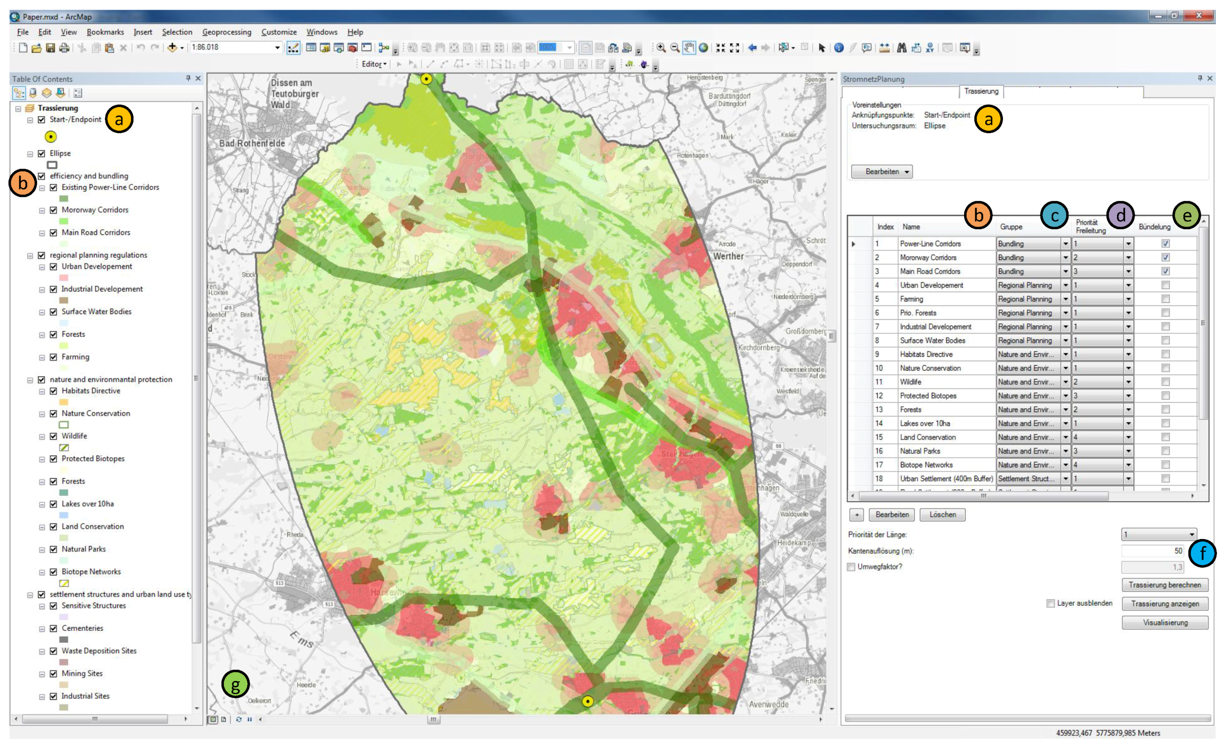
Figure 2 shows the routing criteria definition interface of the designed Add-In. Start and end point as well as the study area are marked from the ArcMap data frame (see Figure 2ⓐ), arbitrary polygon feature layers from the ArcMap data frame can be used (after optional preprocessing using ArcMap functionalities) to define different impacts on the current planning project (see Figure 2ⓑ). Feature layers are classified into an arbitrary amount of criteria categories (see Figure 2ⓒ. Inter group priority values are assigned to the criteria layers defining a weighting of the criteria within its criteria group (see Figure 2ⓓ). Criteria layers with positive impact are marked as bundling criteria (see Figure 2ⓔ) and parameters for the graph creation process like the edge length (see Figure 2ⓕ) can be defined. Criteria layers are visualised in the ArcMap map view (see Figure 2ⓖ).

Solution space grows with the number of criteria and graph edges in an exponential manner, such that an interactive visualisation tool (Section 3.5) is designed to help navigate the solution space by setting constraints on objectives according to varying subjective preferences. Thus, identifying sets of alternative routings based on varying preferences. The interactive visualisation tool is implemented as part of the ArcMap Add-In.

3.2. Modelling of Optimisation Criteria

To support power-line planning, quantifiable evaluation functions are developed, in which planning, ecological and economic decision criteria are considered. The central criteria that are evaluated according to the recommended planning procedure [5] are directly derived from the legal and planning frameworks of land use regulation in Germany. The basic notion is to minimise negative impacts on all assets worth protecting. To date, planning and ecological criteria already implemented comprise distance functions to human settlements, vulnerable commercial and public infrastructures as well as forests, nature reserves, nature parks, special areas of conservation, and landscape protection areas. Additional criteria cover the possibilities of shared alignments with other regional line based infrastructures such as buffers of existing power-lines or motorways. All of these input criteria are based on polygonal spatial structures. Furthermore, evaluation criteria related to economic and operating efficiency are used, e.g., the length of the transmission line. As a basic principle, the approach is flexible and expendable. Under consideration of data availability and calculating time, it is applicable to new criteria in a straightforward manner.

The study area is supposed to be a polygon of arbitrary shape and the start and end point of a route for the grid expansion project under consideration have to be located inside that polygon. The study area is discretised by creating a grid graph and weights for each edge of the graph are calculated (see Section 3.3). The objective functions, as far as negative impacts are concerned, are modelled as the sum of crossing lengths (in metres) regarding the polygon features modelling the identified criteria (see Section 3.1). Shared alignments with corridors surrounding line-based infrastructures (bundling) are modelled as the sum of crossing lengths (in metres) of regions outside these corridors. Thus, edge weights are defined as the crossing lengths of the edge with the polygonal spatial structures of the criteria under consideration.

3.3. Building the Grid Graph

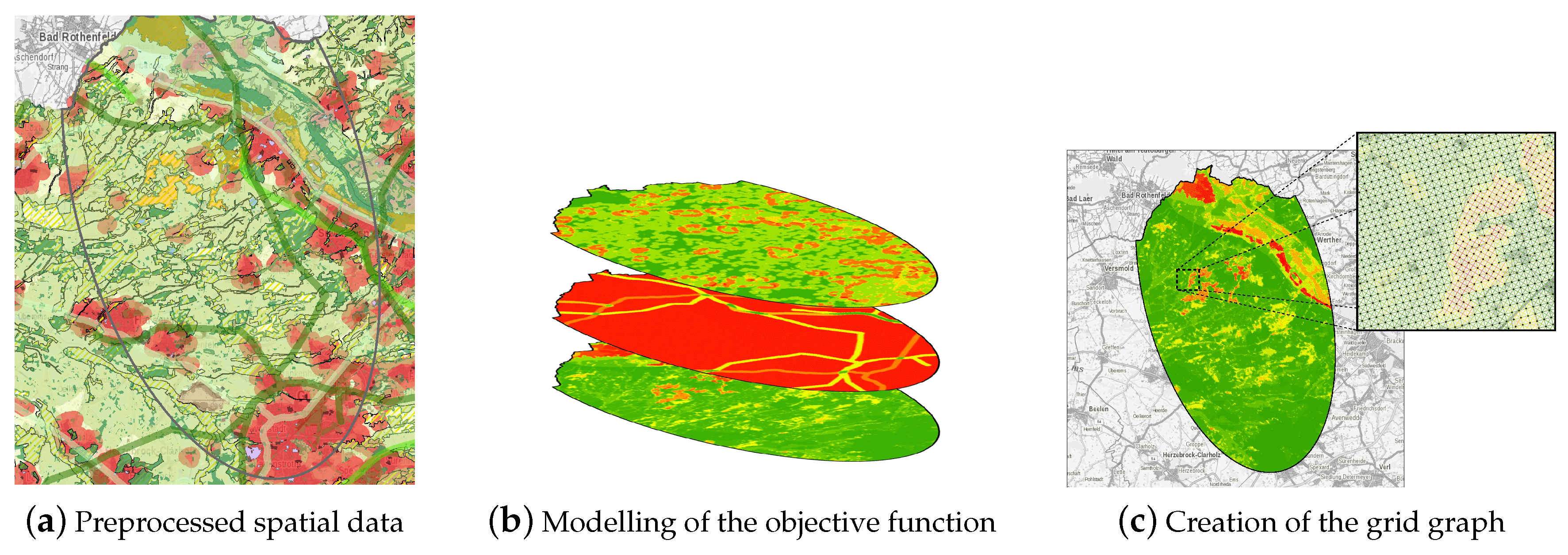
The process of grid creation is illustrated in Figure 3. Criteria modelled as described in the previous section are polygonal spatial structures. The same holds for the study area. Spatial regions with impact on the planning process are processed using GIS. This includes e.g., adjustment of projections, clipping and buffering operations (see Figure 3a). In order to find efficient (in the sense of Pareto-optimisation) routings from the given starting point $\mathbf{s}$ to the end point $\mathbf{t}$ (also referred to as sink), the study area (see Section 3.2) is discretised into a weighted undirected grid graph $G=(V,E)$ (see Figure 3b,c) modelling all possible paths between $\mathbf{s}\in V$ and $\mathbf{t}\in V$. To achieve this, the study area is decomposed into a $N\times M$ raster with a resolution of $r\times r$ metres. The set of vertices V consists of the centres of each raster cell:

$${\mathbf{v}}_{i,j}\in V\subseteq {\mathbb{R}}^2,i\in \{1,\cdots ,N\},j\in \{1,\cdots ,M\},$$

(1)

sampling the study area at $N·M$ points. The set of edges E consists of the associated grid edges

$$E=\{e_{i,j,k,l}=\{{\mathbf{v}}_{i,j},{\mathbf{v}}_{k,l}\}\mid {\mathbf{v}}_{i,j},{\mathbf{v}}_{k,l}\in V,|k-i|=1\vee |l-j|=1\}$$

(2)

(see Figure 3c). Edges are connecting each vertex to its (up to) eight neighbours. Length of grid edges is thus either r or $\sqrt{2}r$ m.

With each edge $e\in E$ of G a vector of real valued positive weights $c\left(e\right)\in {\mathbb{R}}^d$ is incorporated, where d is the number of objectives (see Section 3.2). A path in G is a sequence of edges $(e_1,\cdots ,e_k)$ such that $|e_i\cap e_{i+1}|=1$ for $1\le i\le k-1$. The set of paths between $\mathbf{s}={\mathbf{v}}_{i,j}$ and $\mathbf{t}={\mathbf{v}}_{k,l}$, with $i,k\in \{1,\cdots ,N\}$ and $j,l\in \{1,\cdots ,M\}$, is called ${\mathcal{P}}_{\mathbf{s},\mathbf{t}}$. A path $p\in {\mathcal{P}}_{\mathbf{s},\mathbf{t}}$ has cost

$$\begin{array}{cc}\hfill c\left(p\right)& :=\sum _{e\in p}c\left(e\right)\mathrm{and}\hfill \end{array}$$

(3)

$$\begin{array}{cc}\hfill c\left(P\right)& :=\sum _{p\in P}c\left(p\right),\hfill \end{array}$$

(4)

for a set of paths $P\subseteq {\mathcal{P}}_{\mathbf{s},\mathbf{t}}$. As already stated in Section 3.2, the weight of an edge e, in the context of this work, is modelled as the vector of crossing lengths of e with the polygon(s) associated with each criterion.

Based on the defined graph, a multi-objective optimisation technique is applied to approximate the set of efficient solutions (set of Pareto-optimal paths) from $\mathbf{s}$ to $\mathbf{t}$.

3.4. Multi-Objective Optimisation

The problem is modelled as a Multi-Objective Shortest Path (MOSP) problem. In this, the aforementioned Graph $G=(V,E)$, the start node $\mathbf{s}$ and the sink node $\mathbf{t}$ are given. Furthermore, a multi-objective edge-cost function $c:E\to {\mathbb{R}}^d$, $d\in \mathbb{N}$ is given. While in single-objective optimisation there exists only one optimal value, in multi-objective optimisation, there does not exist one path optimising all objectives at once. The goal here is to find the Pareto-front $\mathcal{Y}$, which is the set of minima of $c\left({\mathcal{P}}_{\mathbf{s},\mathbf{t}}\right)$ with respect to the component wise less-or-equal order on vectors. In addition, each point $y\in \mathcal{Y}$ in one Pareto-optimal path p with $c\left(p\right)=y$ is of interest.

Hence, a Pareto-optimal path p is an $\mathbf{s}$-$\mathbf{t}$-path such that there does not exist another $\mathbf{s}$-$\mathbf{t}$-path $p^{\prime }$ with $c\left(p^{\prime }\right)\le c\left(p\right)$ and $c\left(p^{\prime }\right)\ne c\left(p\right)$, or, in other words: the set of Pareto-optimal paths consist of those $\mathbf{s}$-$\mathbf{t}$-paths where the improvement in one objective needs to result in the deterioration of another objective.

In this context, the ideal objective vector ${\mathbf{z}}^{ideal}$ and the nadir objective vector ${\mathbf{z}}^{nad}$ are defined as

$$\begin{array}{cc}\hfill z_i^{ideal}& =\underset{p\in \mathcal{Y}}{min}{c}_i\left(p\right),\hfill \end{array}$$

(5)

$$\begin{array}{cc}\hfill z_i^{nad}& =\underset{p\in \mathcal{Y}}{max}{c}_i\left(p\right),\hfill \end{array}$$

(6)

$i\in \{1,\cdots ,d\}$ defining upper and lower bounds for the values of the objective function of the Pareto-optimal solutions.

It is well known that the size of $\mathcal{Y}$ can be exponential in the input size even for two objectives [27]. Recently, it has also been shown that there does not exist an output-sensitive algorithm also for the case of two objectives [28]. Since the graphs investigated in this work are very large, the Pareto-front is approximated. The utilised algorithms are implemented based on the work by Bökler [37], i.e., an $(1+\epsilon )$-approximation of the Pareto-frontier is calculated (Fully Polynomial Time Approximation Scheme (FPTAS)).

3.5. Designing an Interactive Visualisation System

The number of Pareto-optimal solutions is typically large (see Section 3.4) and analysis in the spatial domain not suitable without defining constraints to limit the number of solutions according to different preferences. Hence, the aforementioned two-phase process is proposed. First, the Pareto-front is calculated approximately, building the pool of considerable solutions (server side). Afterwards, a custom designed graphical widget is used to set constraints on the set of objectives (criteria). Spatial characteristics of the resulting subsets (of the solution space) are visualised with established GIS.

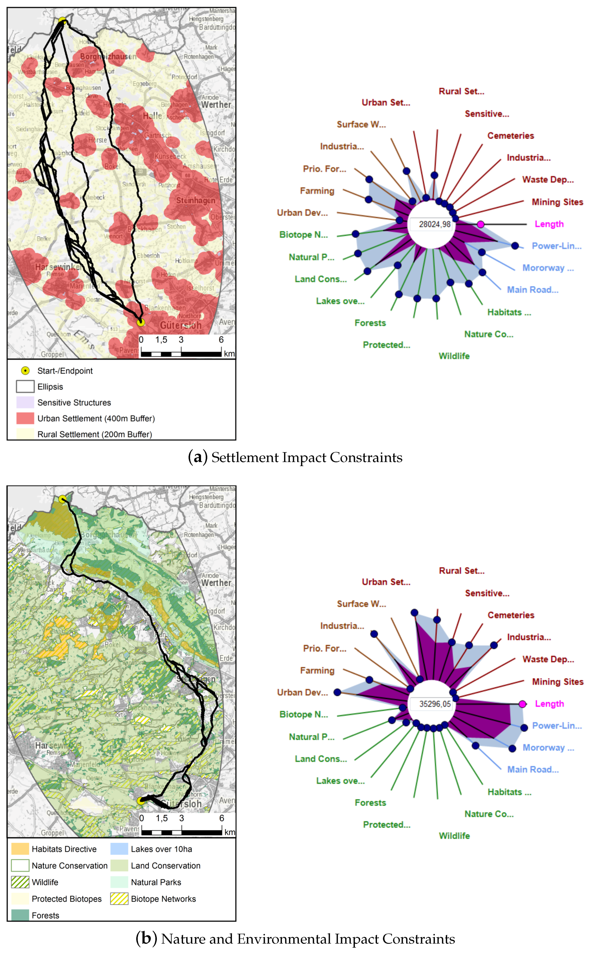
A constraint is set by limiting the maximum allowed cost value for one or more criteria in the set of Pareto-optimal solutions. For this purpose, an add-in for the ArcMap GIS (see Section 3.1) is implemented. A custom-designed user interface is built to navigate through the set of Pareto-optimal solutions interactively. By designing a graphical control element similar to a star plot (or spider plot) [38] like slider arrangement (see Figure 4a,c), evaluation of different sets of constraints is supported. Setting a constraint on the objective function for a specific criterion is realised by intuitively restricting the regarded axis of the spider plot. The impact of the limitation of the maximum tolerated crossing length is visualised by means of a coloured inner polygon connecting the minimum possible slider positions (crossing lengths) under the current set of constraints (see Figure 4). This supports an intuitive exploration of the solution set. The subset of efficient paths under these constraints are visualised in a map view (see Figure 4b,d). Additionally, statistical surveys for individual paths are presented optionally to compare differences in the objective function values. This supports the efficient exploration of the spatial distribution of sets of possible routings under different constraints.

4. Data

This section gives an overview of the data used to evaluate the purposed decision support system. In Section 4.1, the study area is presented. The aforementioned criteria modelling impacts on settlement, nature, regional planning and efficiency are discussed in Section 4.2.

4.1. Study Area

In order to make the grid expansion manageable, singular planning sections were defined. The study area is part of the planned crucial extra-high voltage line from the north to the south of Germany. The urgent demand for grid expansion in this region is legally declared (§§1 ff. Energy Line Extension Act). The planned expansion project will establish a stable energy transmission between regional centres of western Germany. While there is no specific and legally binding route proposal set yet, the trade-off between different planning scenarios carried out by the transmission line planning tool are shown.

The study area extends from the southern border of Lower Saxony to Gütersloh in North Rhine-Westphalia (NRW). The TSO Amprion [39] plans to remove an existing 220 $\mathrm{k}$$\mathrm{V}$ power-line and replace it with a new 380 $\mathrm{k}$$\mathrm{V}$ high voltage transmission line. Due to urbanisation and natural arising of new rural settlements near the existing power-line, the routing of the new micro corridor needs to be adjusted. The study area is characterised by many sprawled rural areas and agricultural land use. As a natural barrier in the north of the study area is the Teutoburg Forest, which contains large areas of nature reserve that are designated as Special Protected Areas and so protected by the European Habitats Directive [40].

4.2. Criteria

Overall 24 spatial decision criteria are used in this study (see Figure 5). The used criteria cover four major topics: economic efficiency (see Figure 5a), settlement structures and important land use types (see Figure 5d) as well as nature and environmental protection, biodiversity and recreation areas (see Figure 5c) and priority areas of regional planning regulations (see Figure 5b).

Economic efficiency is modelled by minimising the overall length of the planned power-line (see Section 3.3). Since line routing along existing transmission lines, motorways or main roads, which already fragment the landscape is desired, three criteria modelling this bundling effect are taken into account. The so-called bundling effect occurs when routing within a buffer of 200 $\mathrm{m}$ around the centre line of the linear infrastructure under consideration.

Table 1. Evaluated criteria for finding optimised transmission line routes and their impact classes.

Category	ID	Description	Impact Class
bundling with linear infrastructure (+ 200 $\mathrm{m}$ buffer)	$o_1$ $o_2$ $o_3$	concentration along existing power-lines concentration along motorways concentration along main roads	high moderate low
regional planning regulations	$o_4$ $o_5$ $o_6$ $o_7$ $o_8$	priority areas for urban development priority areas for farming priority areas for forestry priority areas for industrial development priority areas for surface water bodies	lowest lowest lowest lowest lowest
nature and environmental protection	$o_9$ $o_{10}$ $o_{11}$ $o_{12}$ $o_{13}$ $o_{14}$ $o_{15}$ $o_{16}$ $o_{17}$	habitats directive areas nature conservation areas protected wildlife areas protected biotopes forests water bodies > 10 $\mathrm{h}\mathrm{a}$ landscape conservation areas natural parks biotope networks	high moderate moderate low low low lowest lowest lowest
settlement structures and urban land use	$o_{18}$ $o_{19}$ $o_{20}$ $o_{21}$ $o_{22}$ $o_{23}$ $o_{24}$	urban settlement areas + 400 $\mathrm{m}$ buffer rural settlement areas + 200 $\mathrm{m}$ buffer sensitive structures (e.g., hospitals) cemeteries industrial sites waste deposition sites mining sites	high high moderate moderate moderate moderate moderate
length	$o_{25}$	length	high

gives an overview of the considered criteria and the classification of their impact on power-line routing. Bundling with existing power-line infrastructure has a high impact on the planning of new routes, while the impact of major roads is moderate and low for main roads. Settlement structures and urban land use is comprised of urban residential areas and rural residential areas. Due to strict regulations (§ 4 of the 26th Federal Emission Control Act (26. BImschV) ‘Ordinance on Electromagnetic Fields’), both criteria have a high impact on power-line routing. Criteria are modelled by creating buffers ( 400 $\mathrm{m}$ for urban residential areas and 200 $\mathrm{m}$ for rural residential areas) for the polygons modelling these criteria. In addition, sensitive structures, cemeteries, industrial sites and waste deposition and mining sites are considered. Impact of these structures is moderate.

Furthermore, nine decision criteria regarding the protection of nature and biodiversity extend the criteria catalogue. They cover nature conservation areas, nature parks, forests worth protecting, protected landscapes and areas protected by the EU Flora–Fauna–Habitat (FFH) directive. Detailed view of the impact classes chosen for these criteria is given in Table 1. A detailed view on these criteria reveals (see Figure 5c) that land conservation, forests, natural parks and biotope networks cover most paths along the direct connection of start point and sink. Thus, it is likely to find most paths crossing the associated areas for multiple kilometres.

Since the level of content within regional development plans (§ 5 Regional Planning Act (ROG) ‘Binding Character of Aims of Comprehensive Regional Planning’) is less detailed, the impacts of these five criteria are set to the lowest.

The spatial data used in this work is originated from the Federal Agency for Cartography and Geodesy that provides a nationwide digital data set of geodetic reference data and basic spatial data [41]. Within this approach, the digital basic landscape model data is used gathered from the Authoritative Topographic-Cartographic Information System of Germany at the lowest reference scale 1:25,000. By transposing the EU-INSPIRE-Directive (Directive 2007/2/EC of the European Parliament and of the Council of 14 March 2007 establishing an Infrastructure for Spatial Information in the European Community (INSPIRE)) into federal law, a wide portfolio of spatial data from NRW was published within an Open Government [42] initiative including the datasets used in this work.

5. Results

For runtime efficiency, objective functions are built for the four criteria categories and the length criterion (see Table 1). Hence, conflicts between aggregated objectives of the criteria in the aforementioned categories are illustrated using multi-criteria optimisation:

The four impact classes are modelled by weights $w_i\in \mathbb{N}$, $i\in \{1,2,3,4\},w_i=i$, sorted lowest to highest impact. The weighted sum of the three objectives modelling efficiency and bundling are built using these weights. The same applies to the seven criteria modelling settlement structures and urban land use types, the nine criteria modelling nature and environmental protection and the five criteria modelling regional planning regulations. Length of the paths is used as the fifth criterion. This means that optimisation is performed on a five-dimensional objective function built from the weighted sums of crossing lengths for the criteria depicted. The weights correspond to the impact classes defined in common planning procedures.

The beeline from start to end point is $23.31$ $\mathrm{k}$$\mathrm{m}$. The edge length for the grid graph is set to 50 $\mathrm{m}$. Since data for the area of Lower Saxony is not freely available, the ellipse defining the study area is clipped against its borders. The resulting graph has 149,336 vertices and 594,917 edges.

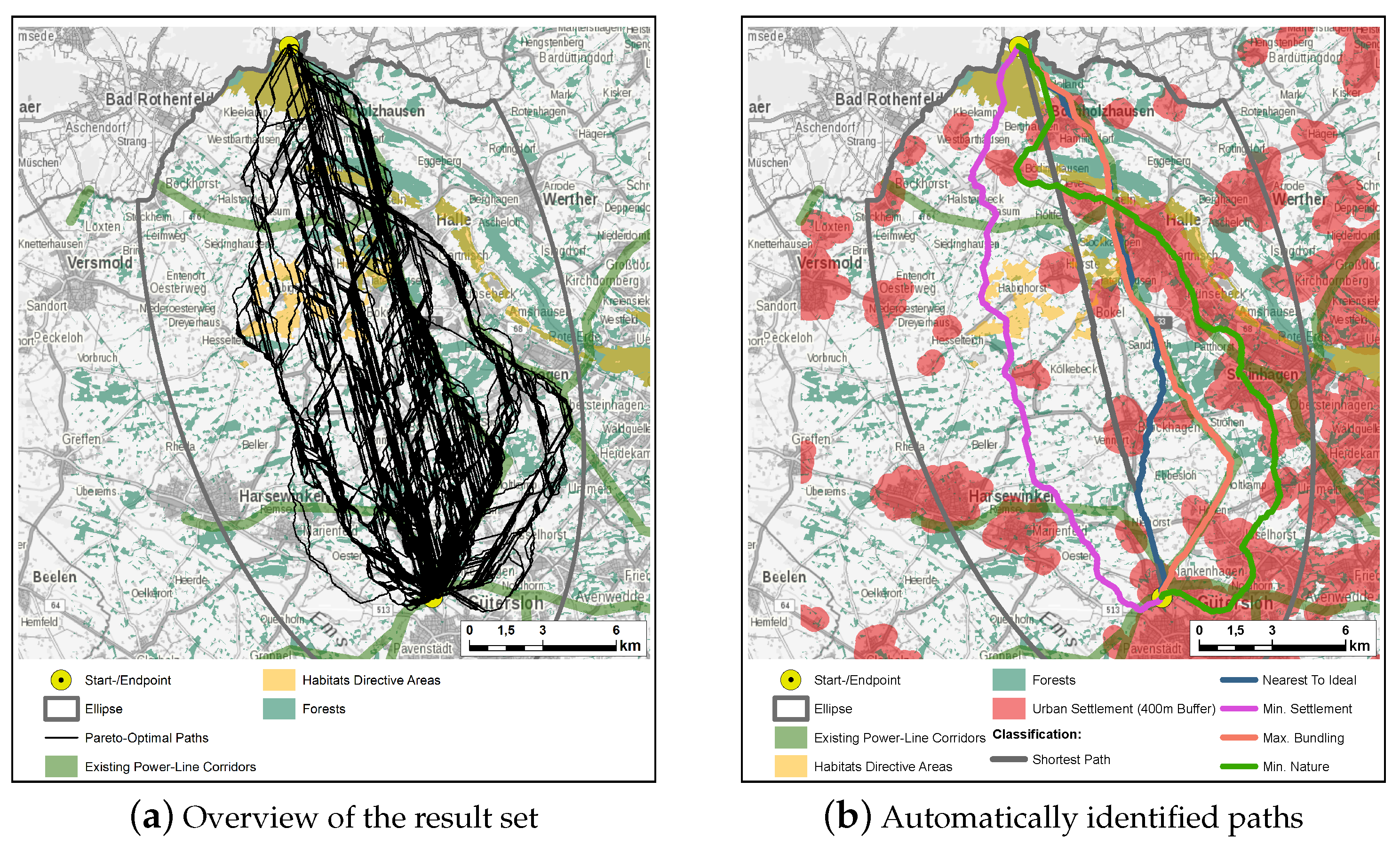
Pareto-optimal paths from start point to sink are calculated using the described criteria categories (see Section 3.2) and parametrisation shown in the previous section. Figure 6 shows the Pareto-front with expected approximation $\epsilon =0.01$ (see Section 3.4). 4,667 Pareto-optimal paths are found.

Table 2. Overview of the resulting cost values for the 4667 Pareto-optimal solutions. Groups $g_1,\cdots ,g_4$ are weighted sums of the criteria depicted in Table 1. $g_5$ represents the lengths of the paths and thus equals $o_{25}$ (see Table 3). Note: $g_1$ is a bundling criterion and thus represents the accumulated lengths along which no linear infrastructure corridors are crossed.

	${\mathit{g}}_1$	${\mathit{g}}_2$	${\mathit{g}}_3$	${\mathit{g}}_4$	${\mathit{g}}_5$
mean	262,215.54	135,263.14	94,531.76	94,083.08	27,052.36
std	40,486.08	8393.63	27,074.91	38,241.67	1678.49
min	176,490.00	118,364.00	34,113.70	25,723.70	23,672.79
25%	232,537.00	129,646.00	74,141.05	64,968.20	25,929.22
50%	265,687.00	133,836.00	94,012.90	87,675.10	26,767.26
75%	289,193.50	139,407.00	112,216.50	115,919.00	27,881.48
max	367,991.00	180,637.00	192,218.00	247,791.00	36,127.42

shows a statistical summary for the five objectives optimised. $g_1,\cdots ,g_4$ are weighted sums of the category groups presented in Table 1. $g_5$ is the length criterion. Section 5.1 shows solutions minimising each of the optimisation criteria and the distance to an approximation of the ideal point. These paths are identified in objective space. In Section 5.2, the interactive approach using the designed interaction system is presented. Here, costs of solutions are analysed according to the 25 objectives defined in Section 3.2.

Table 3. Overview of the resulting crossing lengths for the 4667 Pareto-optimal solutions (corresponding to 12 of the 25 criteria). All values are in metres. Note: $o_1$ is a bundling criterion and thus represents the length along which no linear infrastructure corridors (existing power-lines) are crossed.

	${\mathit{o}}_1$	${\mathit{o}}_9$	${\mathit{o}}_{10}$	${\mathit{o}}_{12}$	${\mathit{o}}_{13}$	${\mathit{o}}_{15}$	${\mathit{o}}_{17}$	${\mathit{o}}_{18}$	${\mathit{o}}_{19}$	${\mathit{o}}_{20}$	${\mathit{o}}_{22}$	${\mathit{o}}_{25}$
mean	16,400.10	650.24	814.71	259.98	2861.54	19,135.67	7663.80	6760.39	11,519.39	35.15	670.53	27,052.36
std	6928.15	934.87	867.86	230.42	2288.32	3369.19	3384.64	5043.95	3071.71	58.76	471.50	1678.49
min	77.25	0.00	0.00	0.00	91.75	5920.21	1068.14	736.38	4180.24	0.00	67.17	23,672.79
25%	11,851.90	0.00	243.48	75.00	1011.57	17,226.39	4858.99	3311.09	9263.85	0.00	244.71	25,929.22
50%	17,725.41	250.00	565.56	187.07	2348.32	19,533.72	7667.46	5398.64	11,302.53	14.14	723.30	26,767.26
75%	21,447.03	730.42	1058.01	396.75	3932.75	21,431.00	10,167.91	8057.41	13,985.11	28.28	883.42	27,881.48
max	30,281.46	5652.94	6022.24	1279.33	11,141.00	27,013.01	16,518.35	28,585.28	19,947.25	316.92	4283.53	36,127.42

shows a statistical summary for a subset of these objectives.

The three defined scenarios are intended to illustrate the functionality of the tool. The results obtained are not supposed to be put into action as optimal routing solutions. However, they reflect all extreme planning positions comprehensibly. In reality, planning processes are subject to multi-stage balancing processes in which a reconciliation of interests is achieved. As a result, this generally leads to an accepted compromise solution. Since the planning process has only just begun and is still open, a final criteria selection and a predetermined weighting of the criteria were not considered here. These definitions will be a central part of the further planning process, where other criteria may be selected or weighted differently.

5.1. Automated Identification of Power-Line Routes

Automated identification of routings takes place in objective space. For this purpose, paths with minimal cost in each of the objective function dimensions are chosen. In addition, the path with minimum Euclidean distance to the ideal point (see Section 3.4) is considered. To interpret the subset of efficient paths, edge costs are mapped back to the original 25-dimensional objective function, i.e., crossing lengths based on the original criteria are discussed. The route with maximum bundling with linear infrastructure follows the existing power-line corridor along nearly the whole path (except for 77 $\mathrm{m}$ of $27.3$ $\mathrm{k}$$\mathrm{m}$). Accumulated impact on environmental protection areas is high with $47.38$ $\mathrm{k}$$\mathrm{m}$ (more than one protected area could occupy the same spatial region). A detailed look on the environmental criteria shows that the impact on habitats directive (441 $\mathrm{m}$), nature conservation (304 $\mathrm{m}$) and protected biotopes (218 $\mathrm{m}$) is below the mean values of the approximated Pareto-front ($650.24$ $\mathrm{m}$, $814.71$ $\mathrm{m}$, $259.98$ $\mathrm{m}$, see Table 3). Therefore, this could be considered the most cost-effective route. The shortest route has a length of $23.673$ $\mathrm{k}$$\mathrm{m}$ but could not be considered a real option since it shows nearly no potential for bundling with linear infrastructure. Crossing of urban settlement area buffers on $4.76$ $\mathrm{k}$$\mathrm{m}$ is below the mean value, but rural settlement area buffers are crossed for $13.63$ $\mathrm{k}$$\mathrm{m}$ and natural and environmental protection areas are crossed along $42.77$ $\mathrm{k}$$\mathrm{m}$. The route with minimum crossing length with settlement areas crosses urban settlement area buffers only along 759 $\mathrm{m}$ and rural settlement on $4.3$ $\mathrm{k}$$\mathrm{m}$, but shows no bundling potential and its length is 125% of the length of the shortest path. Environmental protection areas are crossed for $47.08$ $\mathrm{k}$$\mathrm{m}$. The path minimising crossing lengths of environmental protection areas ($13.667$ $\mathrm{k}$$\mathrm{m}$) has a high impact on settlement areas (along the whole path) and no bundling potential. The cost of this path is second closest to the nadir point of the approximation (in Euclidean distance), which is the vector of maximum costs in all objectives (cf. Section 3.4). Since the path with minimum distance to the nadir point of the approximation is spatially not significantly different from this path, its discussion is omitted. This shows the limited economical sensibility of this route. Finally, the path with minimum Euclidean distance to the ideal point is discussed. With a length of $26.117$ $\mathrm{k}$$\mathrm{m}$, this path is bundling with existing power-line corridors along $16.5$ $\mathrm{k}$$\mathrm{m}$ (63%), crossing rural settlement area buffers along $4.99$ $\mathrm{k}$$\mathrm{m}$ (only 320 $\mathrm{m}$ more than the optimal path) and $11.93$ $\mathrm{k}$$\mathrm{m}$ along rural settlement, which is near the mean value of all solutions. As far as environmental protection is concerned accumulated crossing length are $39.35$ $\mathrm{k}$$\mathrm{m}$, which is below all aforementioned routes except the route with minimum nature and environmental protection area crossing lengths. Thus, this route can be considered an alternative to the most cost-effective route. Reducing of crossing length of criteria with high environmental impact at the cost of less bundling and thus demanding moderate higher financial effort.

These automatically identified solutions, although showing extremal solutions of the approximated Pareto-front, already give a first impression on the challenges arising in multi-criteria decision-making. To demonstrate the decision support opportunities of the presented approach, the visualisation system is used to interactively identify spatially diverse solutions modelling different preferences.

5.2. Interactive Identification of Power-Line Routes

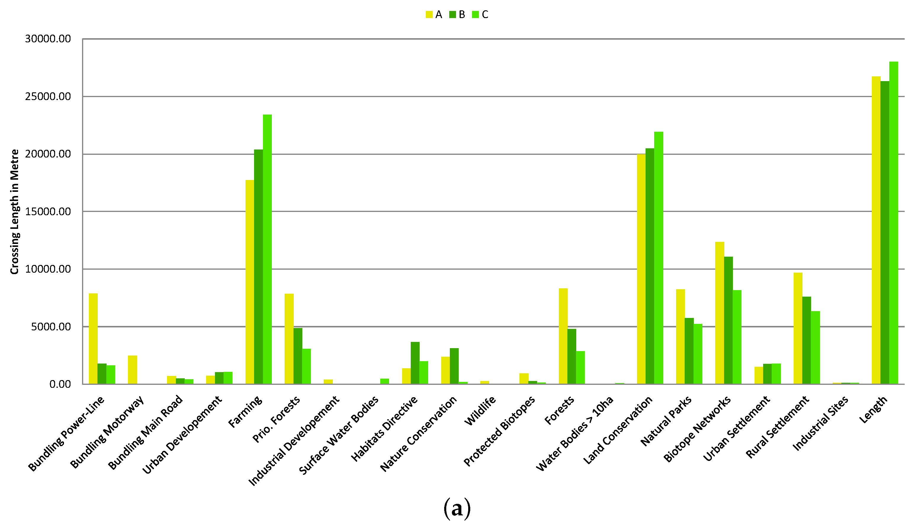
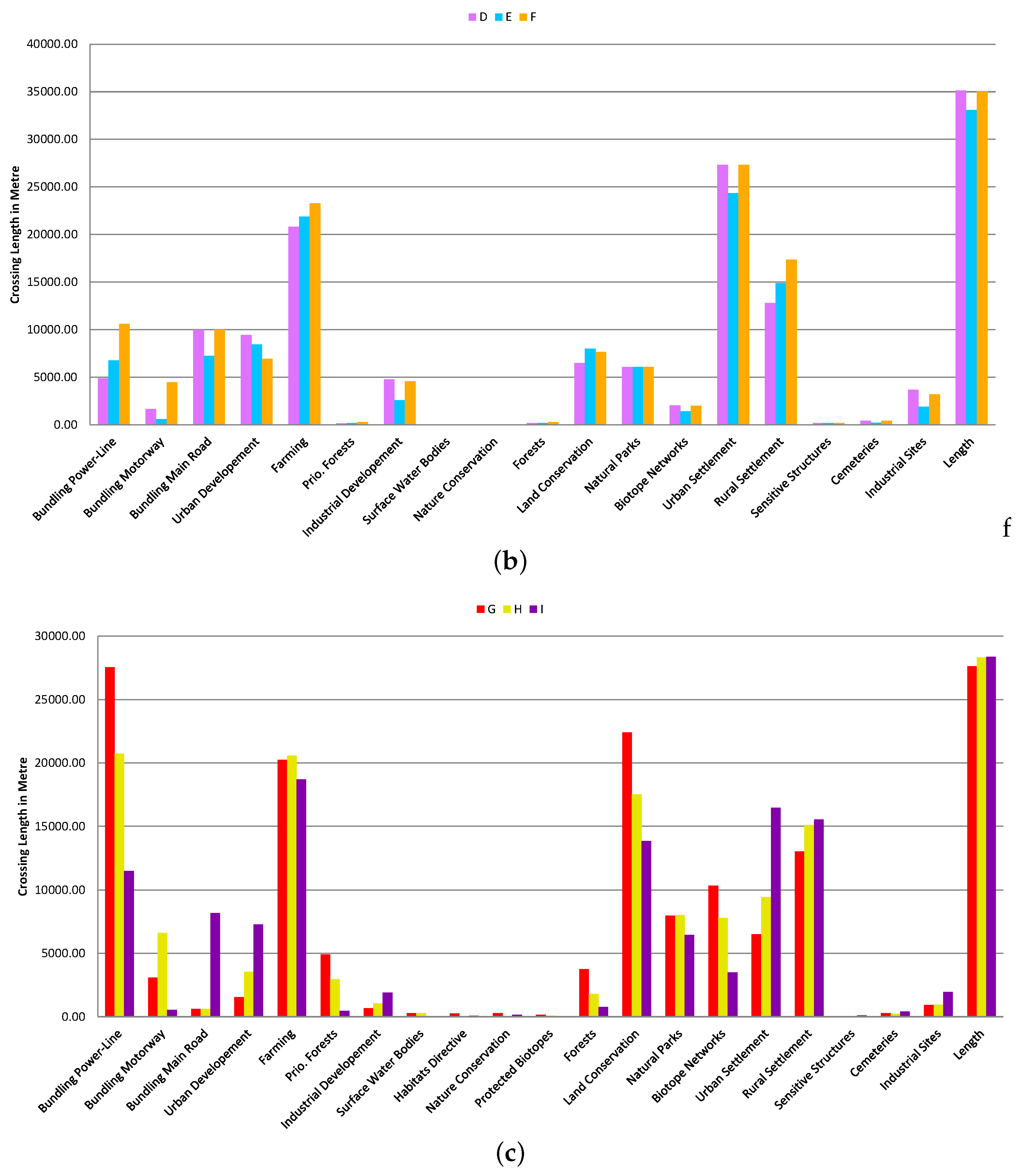
Since planning always means reconciliation of interests, different scenarios can illustrate the broad range of possible conflicts and approaches. In the following sections, three scenarios are identified with the proposed visualisation tool and routes found are discussed. The interactive spider plot is used to navigate the set of Pareto-optimal solutions. For this purpose, edge costs are mapped back to the original 25-dimensional objective function, i.e., crossing length based on the non-agglomerated criteria (see Section 3.2) are discussed. Figure 7 gives an overview of the crossing lengths for the three discussed scenarios and the corresponding alternative routes.

5.2.1. Scenario 1 “Settlement”

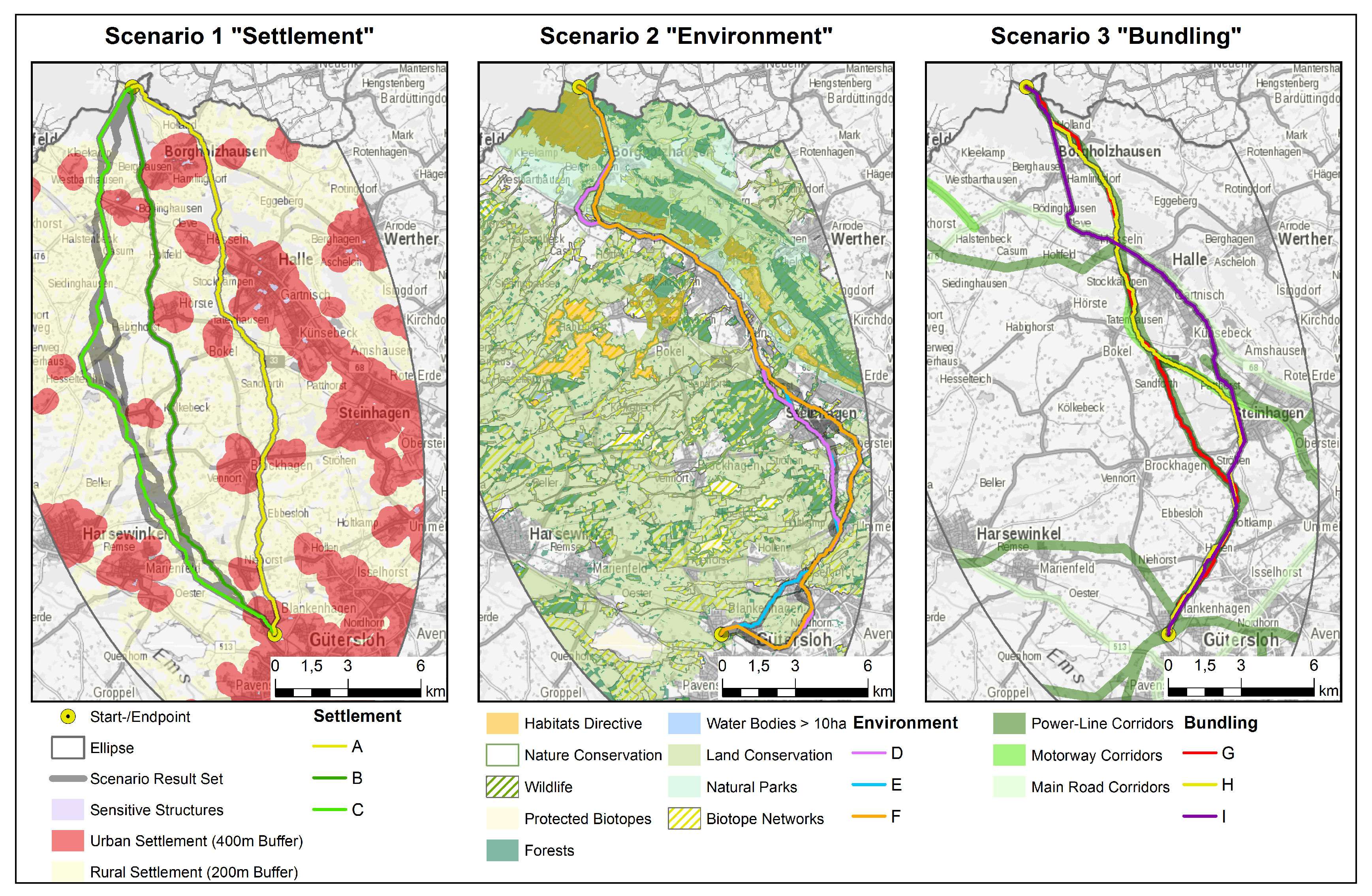
This scenario is created by restricting the set of Pareto-optimal paths by setting maximum crossings of mining sites, waste deposition sites, cemeteries and sensitive structures to zero. Maximum crossing length of urban settlement buffers is restricted to $1.8$ $\mathrm{k}$$\mathrm{m}$ and rural settlement buffer crossing is restricted until three spatial clusters of routes are visible (see Figure 8a and Figure 9 (scenario 1)). Three routes with high spatial variance within this set are highlighted in Figure 9. Route A runs on the east of the start and end point and is $26.74$ $\mathrm{k}$$\mathrm{m}$ long. It shows the biggest bundling potential with $7.8$ $\mathrm{k}$$\mathrm{m}$ along existing power-line corridors. Urban settlement area buffers are crossed along $1.5$ $\mathrm{k}$$\mathrm{m}$ and rural settlement areas along $9.69$ $\mathrm{k}$$\mathrm{m}$. Route B is the shortest in this scenario ($26.32$ $\mathrm{k}$$\mathrm{m}$), reduces rural settlement area crossing by 2 $\mathrm{k}$$\mathrm{m}$ and has no impact on industrial development priority areas. This is achieved at the expense of higher urban settlement buffer crossings ($1.77$ $\mathrm{k}$$\mathrm{m}$), 4 $\mathrm{k}$$\mathrm{m}$ less bundling with existing power-line corridors and 2 $\mathrm{k}$$\mathrm{m}$ less bundling with motorway corridors. As an alternative west of the start and end point, route C (length $28.03$ $\mathrm{k}$$\mathrm{m}$) has minimal crossing of forests with $2.85$ $\mathrm{k}$$\mathrm{m}$. Bundling with linear infrastructure is possible on the same level as for route B.

5.2.2. Scenario 2 “Environment”

In this scenario crossing of habitats directive areas, water bodies greater 10 $\mathrm{h}\mathrm{a}$, protected biotopes and wildlife areas are constrained to zero. The impact on forests is limited to crossing length below 500 $\mathrm{m}$ and crossing length with land conservation areas is limited to 8 $\mathrm{k}$$\mathrm{m}$. The resulting subset of 15 Pareto-optimal paths is shown in Figure 9 (scenario 2). The length of resulting paths range from 33 $\mathrm{k}$$\mathrm{m}$ to 35 $\mathrm{k}$$\mathrm{m}$, which is in the top 1% for all efficient paths (see Table 3). Avoiding crossings of land conservation areas all paths are running in the east of the study area following the B68 (with crossings of existing power-line corridors at up to 29%). The impact on urban settlement areas is high with crossings for 73–79% of the paths’ length. The same holds for priority areas for urban and industrial development. Both crossing lengths are in the top 1% of the whole approximated Pareto-front. Route D is 36 $\mathrm{k}$$\mathrm{m}$ long, has minimal impact on forests (170 $\mathrm{m}$) and follows the B68 on 28% of its length. Route E is the shortest of the routes of this scenario (33 $\mathrm{k}$$\mathrm{m}$), which is 140% of the length of the shortest route in the approximated Pareto-front. The minimal length is achieved through high crossing length with land conservation areas (8 $\mathrm{k}$$\mathrm{m}$). By shortening the route (compared to alternative E) in the north of the study area, bundling with the B68 is only possible on 22% and bundling with existing power-lines is enabled on 20%. Route F (35 $\mathrm{k}$$\mathrm{m}$ long) maximises bundling in this sub set of paths with 30% (power-line), 29% (main roads) and 13% (motorways). This is achieved by two indirections in the east of the study area which enable bundling with the A33 and existing power-line routes following this motorway and the main road B61. These account for the increased length of this alternative.

5.2.3. Scenario 3 “Bundling”

The third scenario optimises for bundling with existing power-line, motorway or main road corridors. The three corresponding routes are visualised in Figure 9 (scenario 3). Since the length of new power-line routings has most impact on cost efficiency, the shortest route could be considered as well. As already stated in the beginning of this section the shortest route is not a real alternative. Alternative G is following the corridor of an existing 220 $\mathrm{k}$$\mathrm{V}$ transmission line (99.7%). It shows a small percentage of bundling with motorways (11%) and main roads (2%). The highest percentage of bundling with motorways is reached by alternative H, which follows motorways at 23% and crosses power-line corridors at 73% (main roads 2%). Alternative I shows highest bundling with main roads. In addition, 29% of the route bundle with existing main road corridors. Power-line corridors are crossed along 40% of the route and motorways are crossed along 2% of the length of this alternative. Impact on land conservation areas is highest with alternative G ($22.4$ $\mathrm{k}$$\mathrm{m}$) and lowest with alternative I ($13.8$ $\mathrm{k}$$\mathrm{m}$). The opposite is true for urban settlement areas ($6.5$ $\mathrm{k}$$\mathrm{m}$, $16.5$ $\mathrm{k}$$\mathrm{m}$) and rural settlement areas (13 $\mathrm{k}$$\mathrm{m}$, $15.5$ $\mathrm{k}$$\mathrm{m}$). This highlights alternative G as the most feasible route, since urban settlement buffer crossings are minimal in this scenario and land conservation areas are unavoidable in this study area without large deviations from the direct connection between start point and sink.

6. Discussion and Conclusions

In this paper, an innovative approach to support decision-making in identifying sets of alternative power-line transmission routings between two connecting points is presented. By using a Pareto-optimisation based approach to solve for practicable routes, conflicts involved in the decision process are emphasised. Subsets of the large set of solutions are created by statistical analysis or by interactively setting constraints. The results highlight the potential value of this method added to the creation of a transparent planning process. The benefit of the presented approach is that subsets of alternative Pareto-optimal routes, created through setting constraints on the maximum allowed crossing distances, allow the definition of scenarios based on subjective assessments. These subsets are created interactively and are presented by the visualisation system, showing the impact of the identified routes on environment and spatial planning. Due to the sensitivity of the German public to grid expansion, the participation and planning process need to provide a high degree of openness and accountability. In addition, there is a high demand of automation of power-line routing methods. By taking both aspects into consideration, this paper presents a new methodological approach of finding optimal power-line routes. By using a Pareto-optimisation technique and the interactive visualisation system, conflicts in the optimisation objectives are illustrated and the complexity of the planners decision-making process is illustrated. This could lead to increased awareness of the challenging power-line routes creation task.

This GeoDesign [43,44] conform approach visualises specific content, and spatially related information of large-scale power-line planning in a comprehensible and interactive form on geographical maps. The ArcMap Add-In allows a collaboration between spatial data, multi-objective optimisation and a graphical user interface. The interactive visualisation (spider-plot) provides dynamic feedback on various planning alternatives and supports planners and stakeholders in the objective analysis and identification of sustainable power-line grid expansions.

Besides utilisation for power-line routing, the presented approach is adaptable to the planning of any line based infrastructure such as roads or pipelines in a straightforward manner. As transmission line planning is affected by both municipal and regional legal frameworks a obligatory elaborate public participation is being carried out by the TSOs. Due to the complexity of transmission line planning, this tool is easy to operate and visually comprehensive, and thus can be most helpful in terms of representing the conflicting objectives of a multi-stage balancing process towards the general public and public agencies.

Future work will concentrate on the modelling and incorporation of different power transmission technologies into the optimisation process. Different criteria sets for overhead lines and underground cables will be considered as well as possible positions for changes from one technology to another. Hence, Pareto-optimal routes considering both technology and the possibility of (multiple) changes within one path will be considered. Additionally, the presented tool should be tested in an actual planning process. Therefore, implementation of an outranking mechanism for the determination of inter-category weightings should be considered.

References

1. Federal Ministry for Economic Affairs and Energy. Fifth “Energy Transition” Monitoring Report; Federal Ministry for Economic Affairs and Energy: Berlin, Germany, 2016.
2. Federal Ministry for Economic Affairs and Energy; Silber Druck oHG. Germany’s New Energy Policy—Heading Towards 2050 with Secure, Affordable and Environmentally Sound Energy; Federal Ministry for Economic Affairs and Energy: Berlin, Germany, 2012.
3. German Energy Agency (Dena). Dena Grid Study II. Integration of Renewable Energy Sources in the German Power Supply System from 2015–2020 with an Outlook to 2025; German Energy Agency: Berlin, Germany, 2011.
4. Federal Network Agency. Grid Expansion in Germany. What You Need to Know; Federal Network Agency: Bonn, Germany, 2016.
5. 50Hertz Transmission GmbH; Amprion GmbH; TenneT TSO GmbH; TransnetBW GmbH. [Application for Federal Sectoral Planning. Sample Application according to § 6 NABEG. Part 1: Coarse and Route Corridors] Antrag auf Bundesfachplanung. Musterantrag nach § 6 NABEG. Teil 1: Grob- und Trassenkorridore; 50Hertz Transmission GmbH; Amprion GmbH; TenneT TSO GmbH; TransnetBW GmbH: Berlin/Dortmund/Bayreuth/Stuttgart, Germany, 2015. [Google Scholar]
6. Monteiro, C.; Ramirez-Rosado, I.J.; Miranda, V.; Zorzano-Santamaria, P.J.; Garcia-Garrido, E.; Fernandez-Jimenez, L.A. GIS Spatial Analysis Applied to Electric Line Routing Optimization. IEEE Trans. Power Deliv. 2005, 20, 934–942. [Google Scholar] [CrossRef]
7. Eroğlu, H.; Aydın, M. Genetic Algorithm in Electrical Transmission Lines Path Finding Problems. In Proceedings of the 2013 8th International Conference on Electrical and Electronics Engineering (ELECO), Bursa, Turkey, 28–30 November 2013; pp. 112–116. [Google Scholar]
8. Douglas, D.H. Least-cost Path in GIS Using an Accumulated Cost Surface and Slopelines. Cartogr. Int. J. Geogr. Inf. Geovis. 1994, 31, 37–51. [Google Scholar] [CrossRef]
9. Saaty, T.L. A Scaling Method for Priorities in Hierarchical Structures. J. Math. Psychol. 1977, 15, 234–281. [Google Scholar] [CrossRef]
10. Saaty, T.L. Multicriteria Decision Making: The Analytic Hierarchy Process: Planning, Priority Setting Resource Allocation; RWS: Chalfont St Peter, UK, 1990. [Google Scholar]
11. Ho, W.; Ma, X. The State-of-the-Art Integrations and Applications of the Analytic Hierarchy Process. Eur. J. Oper. Res. 2018, 267, 399–414. [Google Scholar] [CrossRef]
12. Jeong, J.S.; García-Moruno, L.; Hernández-Blanco, J. A Site Planning Approach for Rural Buildings into a Landscape using a Spatial Multi-criteria Decision Analysis Methodology. Land Use Policy 2013, 32, 108–118. [Google Scholar] [CrossRef]
13. Abudeif, A.; Moneim, A.A.; Farrag, A. Multicriteria Decision Analysis based on Analytic Hierarchy Process in GIS Environment for Siting Nuclear Power Plant in Egypt. Ann. Nucl. Energy 2015, 75, 682–692. [Google Scholar] [CrossRef]
14. Terh, S.H.; Cao, K. GIS-MCDA Based Cycling Paths Planning: A Case Study in Singapore. Appl. Geogr. 2018, 94, 107–118. [Google Scholar] [CrossRef]
15. Mileu, N.; Queirós, M. Integrating Risk Assessment into Spatial Planning: RiskOTe Decision Support System. ISPRS Int. J. Geo-Inf. 2018, 7, 184. [Google Scholar] [CrossRef]
16. Hu, H.; Lin, T.; Wang, S.; Rodriguez, L.F. A cyberGIS Approach to Uncertainty and Sensitivity Analysis in Biomass Supply Chain Optimization. Appl. Energy 2017, 203, 26–40. [Google Scholar] [CrossRef]
17. Houston, G.; Johnson, C. EPRI-GTC Overhead Electric Transmission Line Siting Methodology; Georgia Transmission Corporation: Georgia, CA, USA, 2006. [Google Scholar]
18. Linstone, H.A.; Turoff, M. The Delphi Method: Techniques and Applications; Addison-Wesley: Reading, MA, USA, 1975. [Google Scholar]
19. Schmidt, A.J. Implementing a GIS Methodology for Siting High Voltage Electric Transmission Lines. Pap. Resour. Anal. 2009, 11, 17. [Google Scholar]
20. ArcMap Model Builder. Available online: http://desktop.arcgis.com/de/arcmap/latest/analyze/modelbuilder/what-is-modelbuilder.htm (accessed on 4 May 2018).
21. Bagli, S.; Geneletti, D.; Orsi, F. Routeing of Power Lines through Least-Cost Path Analysis and Multicriteria Evaluation to Minimise Environmental Impacts. Environ. Impact Assess. Rev. 2011, 31, 234–239. [Google Scholar] [CrossRef]
22. Janssen, R.; Herwijnen, M.V.; Beinat, E. Definite-Case Studies and User Manual; Vrije Universiteit Amsterdam/IVM: Amsterdam, The Netherlands, 2003. [Google Scholar]
23. Grassi, S.; Friedli, R.; Grangier, M.; Raubal, M. A GIS-Based Process for Calculating Visibility Impact from Buildings During Transmission Line Routing. In Connecting a Digital Europe Through Location and Place; Huerta, J., Schade, S., Granell, C., Eds.; Springer: Cham, Switzerland, 2014; pp. 383–402. [Google Scholar]
24. Beryozkina, S.; Sauhats, A.; Neimane, V. Designing a Transmission Line Using Pareto Approach. In Proceedings of the IEEE Grenoble PowerTech (POWERTECH) Conference, Grenoble, France, 16–20 June 2013. [Google Scholar]
25. Aissi, H.; Chakhar, S.; Mousseau, V. GIS-Based Multicriteria Evaluation Approach for Corridor Siting. Environ. Plan. B Plan. Des. 2012, 39, 287–307. [Google Scholar] [CrossRef]
26. Medrano, F.A.; Church, R.L. Corridor Location for Infrastructure Development A Fast Bi-objective Shortest Path Method for Approximating the Pareto Frontier. Int. Reg. Sci. Rev. 2014, 37, 129–148. [Google Scholar] [CrossRef]
27. Hansen, P. Bicriterion Path Problems. In Multiple Criteria Decision Making Theory and Application; Fandel, G., Gal, T., Eds.; Lecture Notes in Economics and Mathematical Systems; Springer: Berlin/ Heidelberg, Germay; New York, NY, USA, 1979; Volume 177, pp. 109–127. [Google Scholar]
28. Bökler, F.; Ehrgott, M.; Morris, C.; Mutzel, P. Output-sensitive Complexity of Multiobjective Combinatorial Optimization. J. Multi-Criteria Decis. Anal. 2017, 24, 25–36. [Google Scholar] [CrossRef]
29. Paixao, J.; Santos, J. Labelling Methods for the General Case of the Multiobjective Shortest Path Problem: A Computational Study. In Computational Intelligence and Decision Making; Intelligent Systems, Control and Automation: Science and Engineering; Springer: Dordrecht, The Netherlands, 2009; pp. 489–502. [Google Scholar]
30. Guerriero, F.; Musmanno, R. Label Correcting Methods to Solve Multicriteria Shortest Path Problems. J. Optim. Theory Appl. 2001, 111, 589–613. [Google Scholar] [CrossRef]
31. Bökler, F.; Mutzel, P. Tree-Deletion Pruning in Label-Correcting Algorithms for the Multiobjective Shortest Path Problem. In WALCOM: Algorithms and Computation. WALCOM 2017; Poon, S.H., Rahman, M., Yen, H.C., Eds.; Lecture Notes in Computer Science 10167; Springer: Cham, The Netherlands, 2017; pp. 190–203. [Google Scholar]
32. Erb, S.; Kobitzsch, M.; Sanders, P. Parallel Bi-objective Shortest Paths Using Weight-Balanced B-trees with Bulk Updates. In Experimental Algorithms. SEA 2014; Lecture Notes in Computer Science 8504; Springer: Cham, Switzerland, 2014. [Google Scholar]
33. Warburton, A. Approximation of Pareto Optima in Multiple-Objective Shortest-Path Problems. Oper. Res. 1987, 35, 70–79. [Google Scholar] [CrossRef]
34. Tsaggouris, G.; Zaroliagis, C.D. Multiobjective Optimization: Improved FPTAS for Shortest Paths and Non-Linear Objectives with Applications. Algorithms Comput. 2006, 4288, 389–398. [Google Scholar]
35. ESRI (Environmental Systems Research Institute) ArcGIS Desktop. Available online: http://desktop.arcgis.com/en/arcmap/ (accessed on 20 March 2018).
36. Adamczyk, P.; Smith, P.H.; Johnson, R.; Hafiz, M. REST and Web Services: In Theory and in Practice. In REST: From Research to Practice; Springer: New York, NY, USA, 2011. [Google Scholar]
37. Bökler, F. Output-Sensitive Complexity of Multiobjective Combinatorial Optimization with an Application to the Multiobjective Shortest Path Problem. Ph.D. Thesis, Department of Computer Science, TU Dortmund University, Dortmund, Germany, 2018. [Google Scholar]
38. Chambers, J.; Cleveland, W.; Kleiner, B.; Tukey, P. Graphical Methods for Data Analysis; The Wadsworth Statistics/Probability Series; Duxury: Boston, MA, USA, 1983. [Google Scholar]
39. Amprion GmbH. Available online: https://www.amprion.net/index-2.html (accessed on 6 April 2018).
40. European Habitats Directive. Available online: http://ec.europa.eu/environment/nature/legislation/habitatsdirective/index_en.htm (accessed on 10 April 2018).
41. Federal Agency for Cartography and Geodesy. Digitalc Basic Landscape Model (AAA Modelling); Geodaten der Deutschen Landesvermessung; Federal Agency for Cartography and Geodesy: Frankfurt am Main, Germany, 2016. [Google Scholar]
42. GDI-DE: German Data Infrastructure. Available online: http://www.geoportal.de/EN/GDI-DE/INSPIRE/Legal_Implementation/legal_implementation.html?lang=en (accessed on 6 June 2018).
43. Flaxman, M. Fundamentals of Geodesign. In Peer Reviewed Proceedings of Digital Landscape Architecture 2010 at Anhalt University of Applied Sciences; Wichmann Herbert: Berlin, Germany, 2010; Volume 2, pp. 28–41. [Google Scholar]
44. Steinitz, C. A Framework for Geodesign: Changing Geography by Design; Esri: Redlands, CA, USA, 2012. [Google Scholar]
Figure 1. Overview of the presented workflow: After a set of suitable criteria for a planned grid expansion is identified by start and end point, the modelling of the study area and optimisation criteria is performed by the implemented ArcMap add-in (client). Processed data is transferred to the optimisation server by means of a RESTful web service. A discrete structure (grid graph) is derived from preprocessed spatial data and the optimisation process is started. After an approximation of the Pareto-front (a set of suitable paths) is calculated, results are transferred back to the client for analysis.
Ijgi 07 00258 g001
Figure 2. Criteria generation with the developed ArcMap Add-In: ⓐ definition of start and end point and study area; ⓑ feature layers from the ArcMap data frame added to the list of criteria; ⓒ classified in an arbitrary amount of criteria categories (groups); ⓓ by defining an priority value for each layer, an inter-group weighting of the criterion is achieved; ⓔ criteria with positive impact are flagged as bundling criteria; ⓕ definition of the length of graph edges in metres; ⓖ visualisation of the criteria layers in the ArcMap map view. Data copyright by GeoBasis-DE/BKG 2017.
Ijgi 07 00258 g002
Figure 3. Creation of the grid graph: (a) spatial data is preprocessed using GIS; (b) objective function is modelled (visualisation of three exemplary weight layers) and (c) view of the resulting graph structure. Colour mapping from high values (red) to low values (green) is used.
Ijgi 07 00258 g003
Figure 4. Interactive Visualisation System: (a,c): spider-plot as a graphical control element to support navigation through the set of Pareto-optimal solutions. Criteria are classified into groups (visualised by different colours of sliders and labels). The blue polygon outlines the current slider positions and thus restrictions in the accompanying solution space dimension. The magenta coloured inner polygon shows the minimum possible values for each criterion induced by the current constraints. In the centred circular area of the widget, the current length restriction of the highlighted criterion is shown (in map units, here metre). (b,d): resulting paths for different solution space restrictions are visualised in GIS.
Ijgi 07 00258 g004aIjgi 07 00258 g004b
Figure 5. Criteria used to model the impact of power-line routings in the study area. Criteria are categorised into four categories of protective goods. Data copyright by GeoBasis-DE/BKG 2017. (a) 200 m buffers of linear infrastructures (positive impact); (b) Regional Planning Regulations (negative impact); (c) Nature and Environmental Protection areas (negative impact); (d) Settlement Structures and Urban Land Use (negative impact).
Ijgi 07 00258 g005
Figure 6. (a) overview of the resulting 4667 Pareto-optimal paths; (b) statistically identified paths of interest. Visualisation of the paths minimising each of the five criteria. The path with minimal length is also the path with minimal crossing of priority areas (regional planning regulations). The Nearest-To-Ideal classified path is the one with minimum Euclidean distance to the approximation of the ideal point (see Section 3.4). Data copyright by GeoBasis-DE/BKG 2017.
Ijgi 07 00258 g006
Figure 7. Crossing length for the identified alternatives (cf. Figure 9). Criteria with zero crossings were omitted. (a) scenario 1 “Settlement” with Alternatives A, B, C; (b) scenario 2 “Environment” with Alternatives D, E, F; (c) scenario 3 “Bundling” with Alternatives G, H, I.
Ijgi 07 00258 g007aIjgi 07 00258 g007b
Figure 8. Using the interactive visualisation tool to set constraints on the approximation of the Pareto-front: (a) Minimum Settlement Impact Constraints: Maximum crossing length for mining sites, waste deposition sites, cemeteries and sensitive structures are set to zero. Maximum crossing length of urban settlement buffers is restricted to 1.8 km; (b) Minimum Nature and Environmental Impact Constraints: Crossing of habitats directive areas, water bodies greater than 10 ha, protected biotopes and wildlife areas are constrained to zero. The impact on forests is limited to crossing length below 500 m and crossing length with land conservation areas is limited to 8 km.
Ijgi 07 00258 g008
Figure 9. Visualisation of exemplary results from interaction with the approximated Pareto-front. Data copyright by GeoBasis-DE/BKG 2017.
Ijgi 07 00258 g009