3-D Morphological Change Analysis of a Beach with Seagrass Berm Using a Terrestrial Laser Scanner


Abstract
1. Introduction
2. Materials and Methods
2.1. Study Area
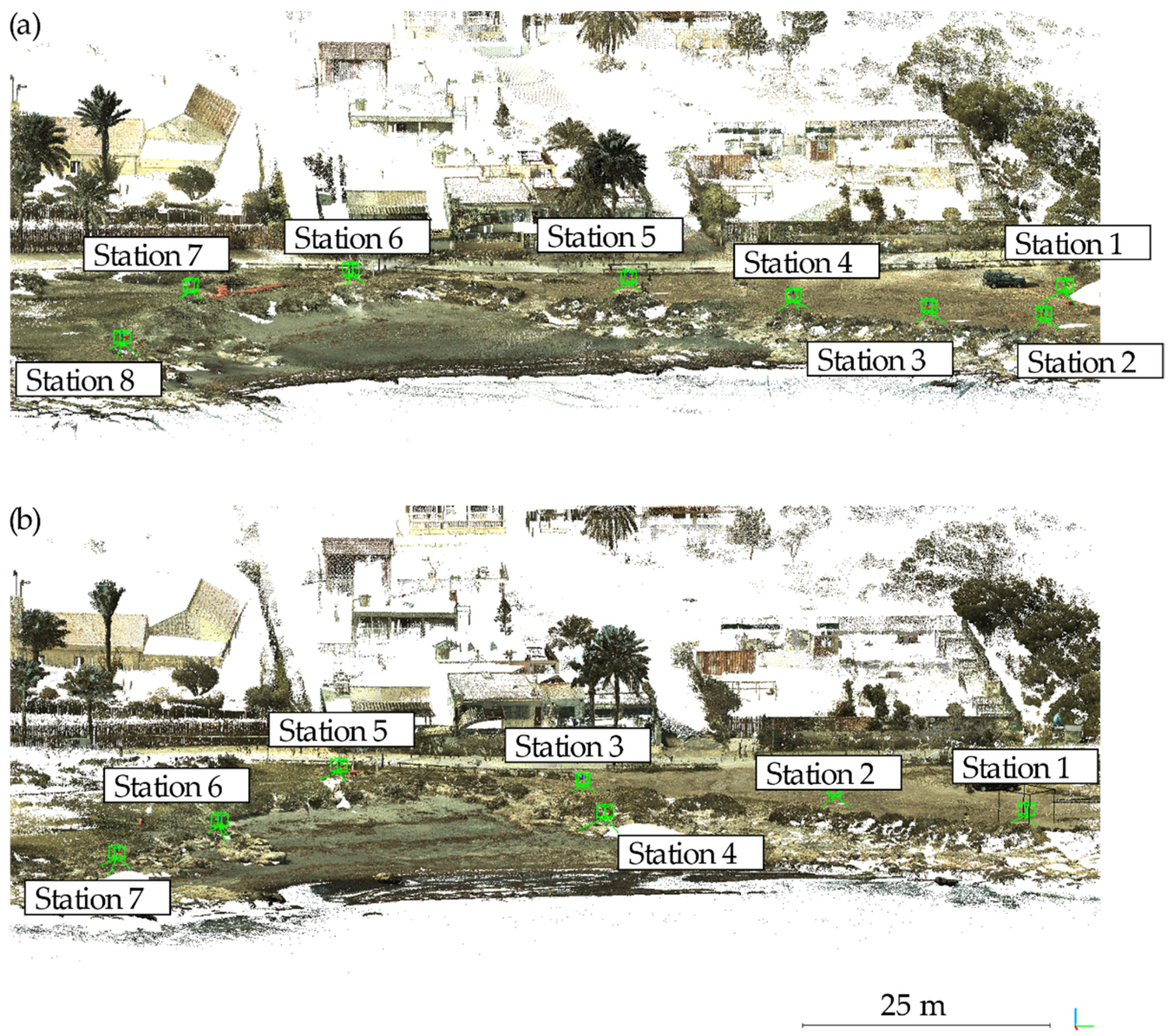
2.2. Data Acquisition
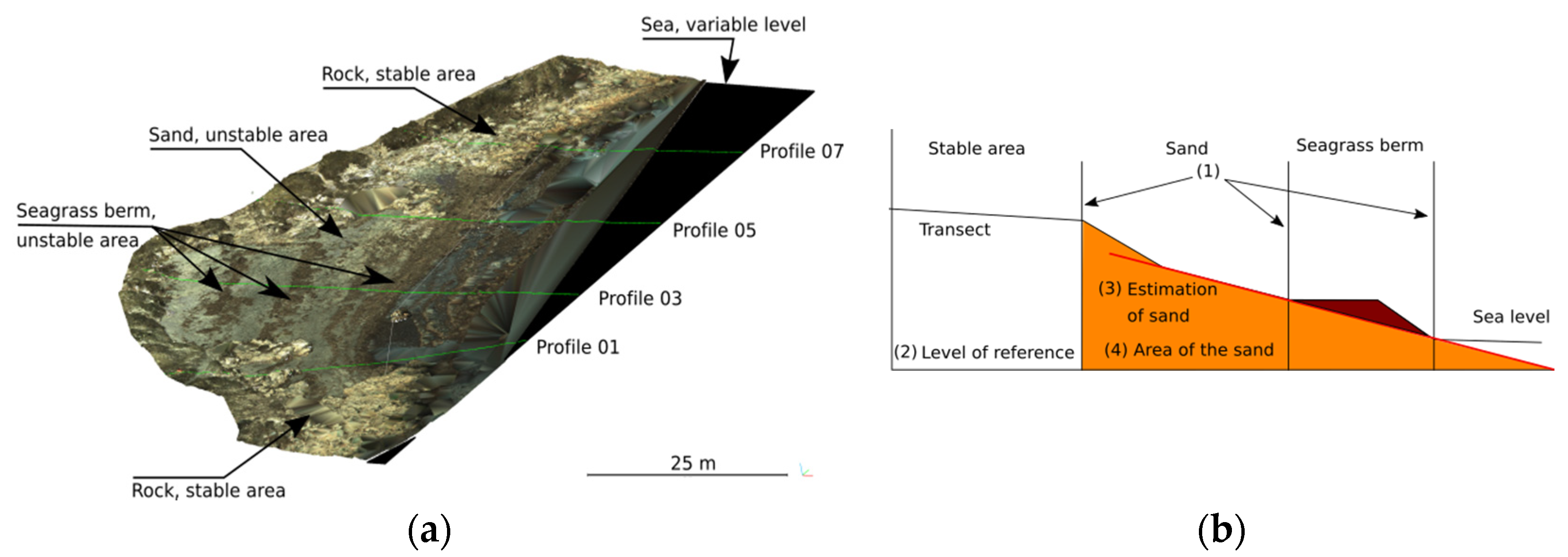
2.3. Data Analysis
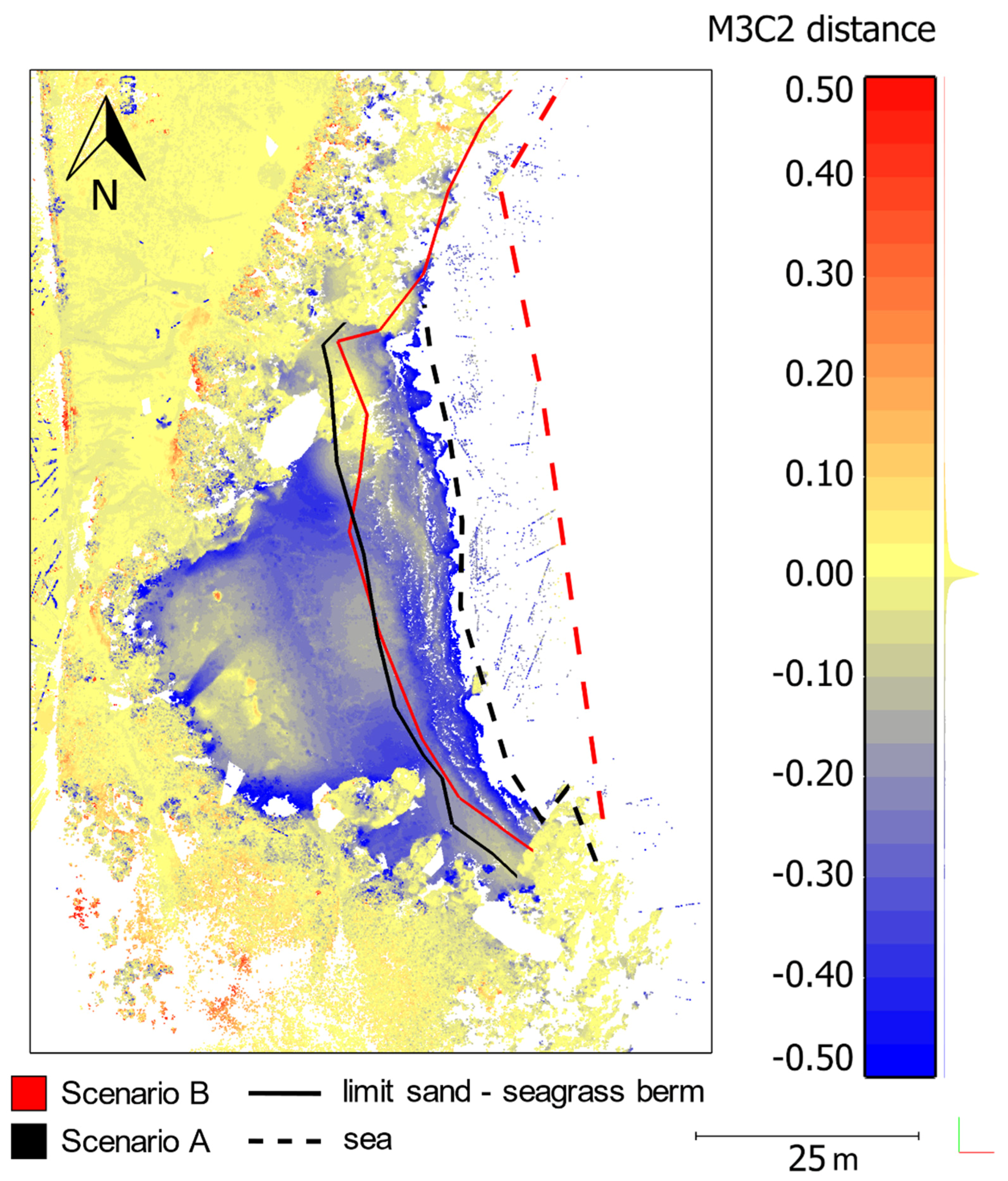
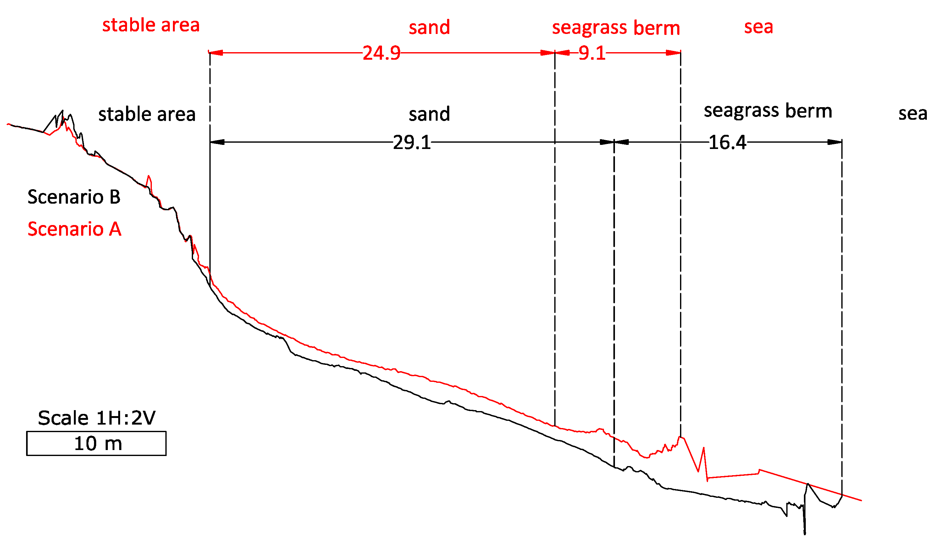
3. Results
4. Discussion
5. Conclusions
Author Contributions
Funding
Acknowledgments
Conflicts of Interest
References
- Short, A.D. The role of wave height, period, slope, tide range and embaymentisation in beach classifications: A review. Rev. Chil. Hist. Nat. 1996, 69, 589–604. [Google Scholar]
- Robertson, A.I.; Lenanton, R.C.J. Fish community structure and food chain dynamics in the surf-zone of sandy beaches: The role of detached macrophyte detritus. J. Exp. Mar. Biol. Ecol. 1984, 84, 265–283. [Google Scholar] [CrossRef]
- Lenanton, R.C.J.; Robertson, A.I.; Hansen, J.A. Nearshore accumulations of detached macrophytes as nursery areas for fish. Mar. Ecol. Prog. Ser. 1984, 9, 51–57. [Google Scholar] [CrossRef]
- Van der Merwe, D.; McLachlan, A. Significance of free-floating macrophytes in the ecology of a sandy beach surf zone. Mar. Ecol. Prog. Ser. 1987, 38, 53–63. [Google Scholar] [CrossRef]
- Orr, K.K.; Wilding, T.A.; Horstmeyer, L.; Weigl, S.; Heymans, J.J. Detached macroalgae: Its importance to inshore sandy beach fauna. Estuar. Coast. Shelf Sci. 2014, 150, 125–135. [Google Scholar] [CrossRef]
- Boudouresque, C.F.; Meinesz, A. Découverte de L'herbier de Posidonies; Cahiers Parc National de Port-Cros: Gardanne, France, 1982. [Google Scholar]
- Simeone, S.; De Falco, G. Posidonia oceanica banquette removal: Sedimentological, geomorphological and ecological implications. J. Coast. Res. 2013, 65, 1045–1050. [Google Scholar] [CrossRef]
- Ochieng, C.A.; Erftemeijer, P.L. Accumulation of seagrass beach cast along the Kenyan coast: A quantitative assessment. Aquat. Bot. 1999, 65, 221–238. [Google Scholar] [CrossRef]
- Boudouresque, C.F.; Jeudy de Grissac, A. L’herbier à Posidonia oceanica en Méditerranée: Les interactions entre la plante et le sédiment. J. Rech. Océanogr. 1983, 8, 99–122. [Google Scholar]
- Jeudy de Grissac, A. Effets des herbiers à Posidonia oceanica sur la dynamique marine et la sedimentology littorale. In International Workshop on Posidonia oceanica Meadows; Boudouresque, C.F., Jeudy de Grissac, A., Oliver, J., Eds.; GIS Posidonie Publisher: Marseille, France, 1984; pp. 437–443. [Google Scholar]
- Simeone, S.; De Falco, G. Morphology and composition of beach-cast Posidonia oceanica litter on beaches with different exposures. Geomorphology 2012, 151, 224–233. [Google Scholar] [CrossRef]
- Ros, J.; Romero, J.; Ballesteros, E.; Gili, J.M. Diving in Blue Water. The Benthos. In Western Mediterranean; Margalef, R., Ed.; Pergamon Press: London, UK, 1985; pp. 233–295. [Google Scholar]
- Vacchi, M.; De Falco, G.; Simeone, S.; Montefalcone, M.; Morri, C.; Ferrari, M.; Bianchi, C.N. Biogeomorphology of the Mediterranean Posidonia oceanica seagrass meadows. Earth Surf. Process. Landf. 2016, 42, 243–386. [Google Scholar] [CrossRef]
- Mas, J.; Franco, I.; Demestre, M.; Guillén, J.; Murcia, F.J.; Ruiz, J.M. Benthic communities on shallow sedimentary bottoms in the Western Mediterranean. In Atlas of Bedforms in the Western Mediterranean; Guillén, J., Acosta, J., Latino-Chiocci, F., Palanques, A., Eds.; Springer: Basel, Switzerland, 2017; pp. 199–206. [Google Scholar]
- Mateo, M.A.; Sánchez-Lizaso, J.L.; Romero, J. Posidonia oceanica ‘banquettes’: A preliminary assessment of the relevance for meadow carbon and nutrients budget. Estuar. Coast. Shelf Sci. 2003, 56, 85–90. [Google Scholar] [CrossRef]
- Gómez-Pujol, L.; Orfila, A.; Álvarez-Ellacuría, A.; Terrado, J.; Tintoré, J. Posidonia oceanica beach-cast litter in Mediterranean beaches: A coastal videomonitoring study. J. Coast. Res. 2013, 65, 1768–1773. [Google Scholar] [CrossRef]
- Romero, J.; Pergent, G.; Martini, C.; Mateo, M.A.; Regnier, C. The detritic compartment in a Posidonia oceanica meadow: Litter features, decomposition rates, and mineral stocks. Mar. Ecol. 1992, 13, 69–83. [Google Scholar] [CrossRef]
- Ferrandis, E.; Bartolomé, F. Dulces bárbaros del Este y del Oeste (Análisis estadístico de los vientos en la bahía de Alicante). In La Reserva Marina de la Isla Plana o Nueva Tabarca (Alicante), 1st ed.; Ramos-Esplá, A.A., Ed.; Ayuntamiento de Alicante, Universidad de Alicante: Alacant, Spain, 1985; pp. 51–94. [Google Scholar]
- De Falco, G.; Simeone, S.; Baroli, M. Management of beach-cast Posidonia oceanica seagrass on the island of Sardinia (Italy, Western Mediterranean). J. Coast. Res. 2008, 24, 69–75. [Google Scholar] [CrossRef]
- Brock, J.C.; Purkis, S.J. The emerging role of lidar remote sensing in coastal research and resource management. J. Coast. Res. 2009, 53, 1–5. [Google Scholar] [CrossRef]
- Johnson, K.M.; Ouimet, W.B. Rediscovering the lost archaeological landscape of southern New England using airborne light detection and ranging (LiDAR). J. Archaeol. Sci. 2014, 43, 9–20. [Google Scholar] [CrossRef]
- Chiabrando, F.; Spanò, A.; Sammartano, G.; Teppati Losè, L. UAV oblique photogrammetry and lidar data acquisition for 3D documentation of the Hercules Fountain. Virtual Archaeol. Rev. 2017, 8, 83. [Google Scholar] [CrossRef]
- Luo, S.; Wang, C.; Xi, X.; Pan, F.; Peng, D.; Zou, J.; Nie, S.; Qin, H. Fusion of airborne LiDAR data and hyperspectral imagery for aboveground and belowground forest biomass estimation. Ecol. Indic. 2017, 73, 378–387. [Google Scholar] [CrossRef]
- Westoby, M.J.; Brasington, J.; Glasser, N.F.; Hambrey, M.J.; Reynolds, J.M. ‘Structure-from-Motion’ photogrammetry: A low-cost, effective tool for geoscience applications. Geomorphology 2012, 179, 300–314. [Google Scholar] [CrossRef]
- Riquelme, A.; Cano, M.; Tomás, R.; Abellán, A. Identification of rock slope discontinuity sets from laser scanner and photogrammetric point clouds: A comparative analysis. Procedia Eng. 2017, 191, 838–845. [Google Scholar] [CrossRef]
- Klemas, V. Beach profiling and LIDAR bathymetry: An overview with case studies. J. Coast. Res. 2011, 27, 1019–1028. [Google Scholar] [CrossRef]
- Andrews, B.D.; Gares, P.; Colby, J.D. Techniques for GIS modeling of coastal dunes. Geomorphology 2002, 48, 289–308. [Google Scholar] [CrossRef]
- Woolard, J.W.; Colby, J.D. Spatial characterization, resolution, and volumetric change of coastal dunes using airborne LIDAR: Cape Hatteras, North Carolina. Geomorphology 2002, 48, 269–287. [Google Scholar] [CrossRef]
- Saye, S.E.; Van der Wal, D.; Pye, K.; Blott, S.J. Beach–dune morphological relationships and erosion/accretion: An investigation at five sites in England and Wales using LIDAR data. Geomorphology 2005, 72, 128–155. [Google Scholar] [CrossRef]
- Lorenzo-Lacruz, J.; Pons, G.X.; Mir-Gual, M. Mapeo semi-automatizado de campos de dunas mediante tecnología LIDAR: Aplicación en el sistema dunar de Sa Canova de Artá (Mallorca). IX Jornadas de Geomorfología Litoral 2017, 17, 135–138. [Google Scholar]
- Sallenger, A.H., Jr.; Krabill, W.B.; Swift, R.N.; Brock, J.; List, J.; Hansen, M.; Holmas, R.A.; Manizade, S.; Sontag, J.; Meredith, A.; et al. Evaluation of airborne topographic lidar for quantifying beach changes. J. Coast. Res. 2003, 19, 125–133. [Google Scholar]
- Gares, P.A.; Wang, Y.; White, S.A. Using LIDAR to monitor a beach nourishment project at Wrightsville Beach, North Carolina, USA. J. Coast. Res. 2006, 22, 1206–1219. [Google Scholar] [CrossRef]
- Nicoletti, L.; Valentini, E.; Targusi, M.; La Valle, P.; Fornari, A.; Taramelli, A. Characterisation of Posidonia oceanica meadows using both hyperspectral and LIDAR data: A new approach. Biol. Mar. Mediterr. 2010, 17, 173–174. [Google Scholar]
- Simeone, S.; De Muro, S.; De Falco, G. Seagrass berm deposition on a Mediterranean embayed beach. Estuar. Coast. Shelf Sci. 2013, 135, 171–181. [Google Scholar] [CrossRef]
- Simeone, S.; De Falco, G.; Quattrocchi, G.; Cucco, A. Morphological changes of a Mediterranean beach over one year (San Giovanni Sinis, western Mediterranean). J. Coast. Res. 2014, 70, 217–222. [Google Scholar] [CrossRef]
- González-Correa, J.M.; Torquemada, Y.F.; Lizaso, J.L.S. Long-term effect of beach replenishment on natural recovery of shallow Posidonia oceanica meadows. Estuar. Coast. Shelf Sci. 2007, 76, 834–844. [Google Scholar] [CrossRef]
- Olcina-Cantos, J.; Torres-Alfosea, F.J. Incidencia de los temporales de levante en la ordenación del litoral alicantino. Papeles de Geografía 1997, 26, 109–136. [Google Scholar]
- López, I.; Aragonés, L.; Villacampa, Y. Analysis and modelling of cross-shore profile of gravel beaches in the province of Alicante. Ocean Eng. 2016, 118, 173–186. [Google Scholar] [CrossRef]
- Carrea, D.; Abellán, A.; Humair, F.; Matasci, B.; Derron, M.H.; Jaboyedoff, M. Correction of terrestrial LiDAR intensity channel using Oren–Nayar reflectance model: An application to lithological differentiation. J. Photogramm. Remote Sens. 2016, 113, 17–29. [Google Scholar] [CrossRef]
- Leica Geosystems AG. Leica ScanStation C10 Data Sheet; Leica Geosystems AG: Heerbrugg, Switzerland, 2011. [Google Scholar]
- Besl, P.J.; McKay, N.D. A method for registration of 3-D shapes. IEEE Trans. Pattern Anal. Mach. Intell. 1992, 14, 239–256. [Google Scholar] [CrossRef]
- James, M.R.; Robson, S.; d’Oleire-Oltmanns, S.; Niethammer, U. Optimising UAV topographic surveys processed with structure-from-motion: Ground control quality, quantity and bundle adjustment. Geomorphology 2017, 280, 51–66. [Google Scholar] [CrossRef]
- Leica. Cyclone v9.1. Leica Geosystems. 2016. Available online: http://leica-geosystems.com/products/laser-scanners/software/leica-cyclone (accessed on 24 November 2017).
- CloudCompare (Version 2.8) [GPL Software]. 2018. Available online: http://www.cloudcompare.org/ (accessed on 19 June 2018).
- Brodu, N.; Lague, D. 3D point cloud classification of complex natural scenes using a multi-scale dimensionality criterion: Applications in geomorphology. J. Photogramm. Remote Sens. 2012, 68, 121–134. [Google Scholar] [CrossRef]
- Lai, P.; Samson, C.; Bose, P. Visual enhancement of 3D images of rock faces for fracture mapping. Int. J. Rock Mech. Min. Sci. 2014, 72, 325–335. [Google Scholar] [CrossRef]
- Boudoresque, C.F.; Ponel, P.; Astruch, P.; Barcelo, A.; Blanfuné, A.; Geoffroy, D.; Thibaut, T. The high heritage value of the Mediterranean sandy beaches, with a particular focus on the Posidonia oceanica “banquettes”: A review. Sci. Rep. Port-Cros Natl. Park 2017, 31, 23–70. [Google Scholar]
- Burvingt, O.; Masselink, G.; Russell, P.; Scott, T. Beach response to consecutive extreme storms using LiDAR along the SW coast of England. J. Coast. Res. 2016, 75, 1052–1056. [Google Scholar] [CrossRef]
- Pietro, L.S.; O’neal, M.A.; Puleo, J.A. Developing terrestrial-LIDAR-based digital elevation models for monitoring beach nourishment performance. J. Coast. Res. 2008, 24, 1555–1564. [Google Scholar] [CrossRef]
- Zhou, G. Coastal 3D change pattern analysis using LIDAR series data. In Remote Sensing of Coastal Environments; Wang, Y., Ed.; CRC Press: Boca Raton, FL, USA, 2010; pp. 103–120. [Google Scholar]
- Stockdonf, H.F.; Sallenger, A.H., Jr.; List, J.H.; Holman, R.A. Estimation of shoreline position and change using airborne topographic lidar data. J. Coast. Res. 2002, 18, 502–513. [Google Scholar]
- Young, A.P.; Ashford, S.A. Application of airborne LIDAR for seacliff volumetric change and beach-sediment budget contributions. J. Coast. Res. 2006, 22, 307–318. [Google Scholar] [CrossRef]
- Aragonés, L.; García-Barba, J.; García-Bleda, E.; López, I.; Serra, J. Beach nourishment impact on Posidonia oceanica: Case study of Poniente Beach (Benidorm, Spain). Ocean Eng. 2015, 107, 1–12. [Google Scholar] [CrossRef]
- López, I.M.; López, M.; Aragonés, L.; Garcia-Barba, J.; López, M.P.; Sánchez, I. The erosion of the beaches on the coast of Alicante: Study of the mechanisms of weathering by accelerated laboratory tests. Sci. Total Environ. 2016, 566, 191–204. [Google Scholar] [CrossRef] [PubMed]
- Pagán, J.I.; Aragonés, L.; Tenza-Abril, A.J.; Pallarés, P. The influence of anthropic actions on the evolution of an urban beach: Case study of Marineta Cassiana Beach, Spain. Sci. Total Environ. 2016, 559, 242–255. [Google Scholar] [CrossRef] [PubMed]
- Pagán, J.I.; López, M.; López, I.; Tenza-Abril, A.J.; Aragonés, L. Causes of the different behaviour of the shoreline on beaches with similar characteristics. Study case of the San Juan and Guardamar del Segura beaches, Spain. Sci. Total Environ. 2018, 634, 739–748. [Google Scholar] [CrossRef] [PubMed]
- Chiva, L.M.; Pagán, J.I.; López, I.; Tenza-Abril, A.J.; Aragonés, L.; Sánchez, I. The effects of sediment used in beach nourishment: Study case El Portet de Moraira beach. Sci. Total Environ. 2018, 628, 64–73. [Google Scholar] [CrossRef] [PubMed]
- Beachmed. Evaluación de Recursos Sedimentarios en Los Fondos Antelitorales de la Comunidad Valenciana; Generalitat Valenciana: Valencia, Spain, 2003. [Google Scholar]


| Profile | L (m) | Scenario A (m2) | Scenario B (m2) | B-A (m2) | (B-A)xL (m3) |
|---|---|---|---|---|---|
| 1 | 20 | 39.33 | 47.13 | 7.8 | 156 |
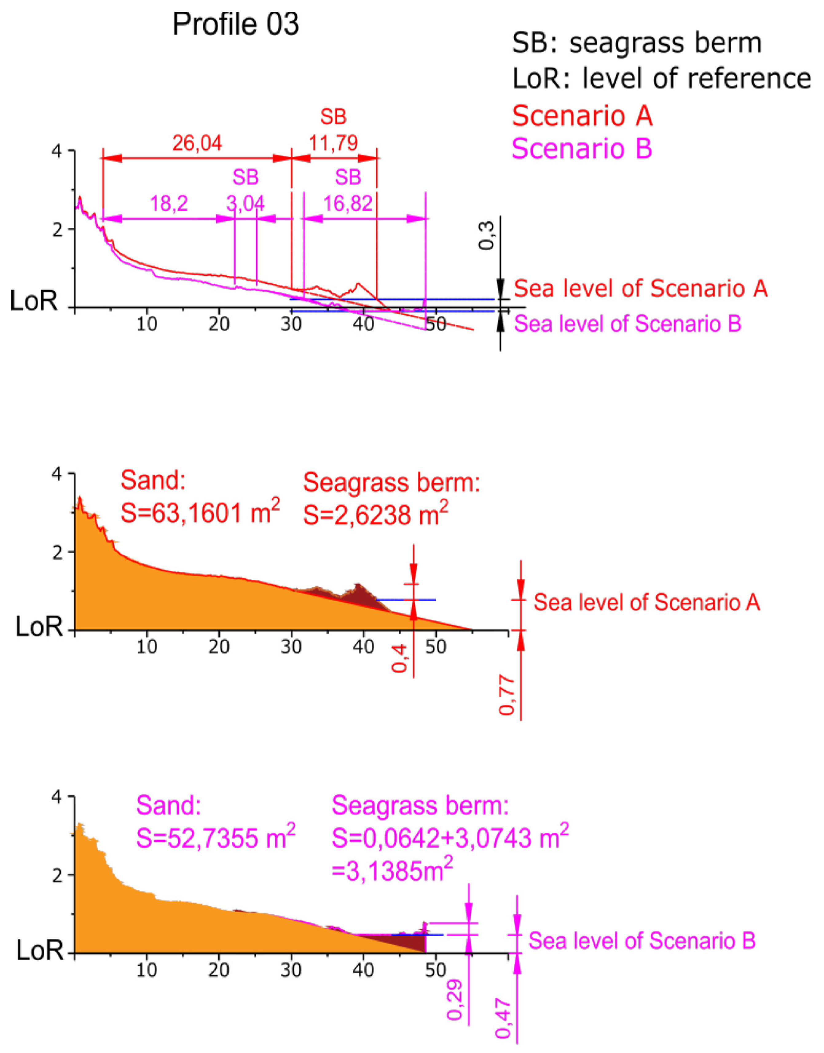
| 3 | 20 | 63.1601 | 52.7355 | −10.4246 | −208.492 |
| 5 | 20 | 50.46 | 43.57 | −6.89 | −137.8 |
| 7 | 20 | 0 | 0 | 0 | 0 |
| TOTAL | −190.292 |
© 2018 by the authors. Licensee MDPI, Basel, Switzerland. This article is an open access article distributed under the terms and conditions of the Creative Commons Attribution (CC BY) license (http://creativecommons.org/licenses/by/4.0/).
Share and Cite
Corbí, H.; Riquelme, A.; Megías-Baños, C.; Abellan, A. 3-D Morphological Change Analysis of a Beach with Seagrass Berm Using a Terrestrial Laser Scanner. ISPRS Int. J. Geo-Inf. 2018, 7, 234. https://doi.org/10.3390/ijgi7070234
Corbí H, Riquelme A, Megías-Baños C, Abellan A. 3-D Morphological Change Analysis of a Beach with Seagrass Berm Using a Terrestrial Laser Scanner. ISPRS International Journal of Geo-Information. 2018; 7(7):234. https://doi.org/10.3390/ijgi7070234
Chicago/Turabian StyleCorbí, Hugo, Adrian Riquelme, Clara Megías-Baños, and Antonio Abellan. 2018. "3-D Morphological Change Analysis of a Beach with Seagrass Berm Using a Terrestrial Laser Scanner" ISPRS International Journal of Geo-Information 7, no. 7: 234. https://doi.org/10.3390/ijgi7070234
APA StyleCorbí, H., Riquelme, A., Megías-Baños, C., & Abellan, A. (2018). 3-D Morphological Change Analysis of a Beach with Seagrass Berm Using a Terrestrial Laser Scanner. ISPRS International Journal of Geo-Information, 7(7), 234. https://doi.org/10.3390/ijgi7070234