Abstract
Spatial group recommendation refers to suggesting places to a given set of users. In a group recommender system, members of a group should have similar preferences in order to increase the level of satisfaction. Location-based social networks (LBSNs) provide rich content, such as user interactions and location/event descriptions, which can be leveraged for group recommendations. In this paper, an automatic user grouping model is introduced that obtains information about users and their preferences through an LBSN. The preferences of the users, proximity of the places the users have visited in terms of spatial range, users’ free days, and the social relationships among users are extracted automatically from location histories and users’ profiles in the LBSN. These factors are combined to determine the similarities among users. The users are partitioned into groups based on these similarities. Group size is the key to coordinating group members and enhancing their satisfaction. Therefore, a modified k-medoids method is developed to cluster users into groups with specific sizes. To evaluate the efficiency of the proposed method, its mean intra-cluster distance and its distribution of cluster sizes are compared to those of general clustering algorithms. The results reveal that the proposed method compares favourably with general clustering approaches, such as k-medoids and spectral clustering, in separating users into groups of a specific size with a lower mean intra-cluster distance.
1. Introduction
The rapid development of the mobile Internet has enabled users to share their information on mobile phones. Recent advancements in location acquisition and wireless communication technologies have led to the development of location-based social networks (LBSNs). Location data bridge the gap between the physical and digital worlds and provide a deeper understanding of user preferences and behaviour. There are many real LBSN systems, such as Foursquare (www.foursquare.com), Gowalla, and GeoLife [1,2]. Moreover, recent studies on identifying user locations from traditional social networks, such as Twitter (www.twitter.com), have contributed to the development of various ways to obtain such information from real-world LBSNs [3].
In location-based social networks (LBSNs), users share information about their locations, the places they visit, and their movement alongside with other social information. Visits are reported explicitly (by user check-ins in known venues and locations) or implicitly by allowing for smartphone applications to report visited locations to the LBSN. This information is then shared with other users who are socially related (e.g., friends) [4].
With the development of social networks and online communities, an increasing number of activities are being performed in groups [5]. Web and information technologies should make our everyday life easier and more comfortable. In this regard, a recommender system contributes to reducing the information overload problem. Standard recommendation approaches, which have been used in various domains, mostly focus on a single user. However, there are many situations when the user interacts socially, with or without restraints. In some situations, we want to interact socially, (e.g., having dinner with friends), while in other situations we are forced to participate in groups, (e.g., mass transit). We are also a part of much larger social groups which form and adjust our behaviour and norms [6]. Nowadays, less attention is paid to social aspects of individuals and groups as units. Incorporating users’ social links based on social networks and user personalities provides both the recommendation and grouping process with more realistic information modelling [7].
To support recommendation in social activities, group recommender systems were developed. LBSNs provide rich content (location, time-stamps) and social network information, which can help in modeling group dynamics for group recommendations [8]. There are cases where a group of people participates in a single activity. For instance, visiting a restaurant or a tourist attraction, watching a movie and selecting a holiday destination are examples of recommendations that are well suited for groups of people. Spatial group recommender systems provide suggestions about places when more than one person is involved in the recommendation process. Groups are composed of members with similar preferences that can have a similar recommendation. The more preferences that group members have in common, the more easily the group recommender system can suggest items that result in higher levels of satisfaction among the members. When groups do not already exist, another key aspect of group recommendation is related to groups identification [9]. Since the determination and coordination of group members is very time-consuming, in this paper an automatic selection process based on an unsupervised clustering approach is used to partition users into groups of a specific size with the most similar members.
The most popular approach for partitioning users into groups is the clustering algorithm. It is a fundamental research topic in data mining and is widely used for various applications in scientific fields such as artificial intelligence, statistics and social sciences. The objective of clustering is to partition the original data points into a number of groups so that data points within the same cluster are similar to each other, but are different from those in other clusters [10]. As the main objective of this study is to create groups of a specific size, there are several factors to be accounted for in similarity estimations. These are user preferences, social relationships, an individual’s free days and spatial proximity, and these are also the key factors in creating a favourable space and maximizing user satisfaction. To achieve this aim, a modified k-medoids algorithm is developed and applied to user similarities, and consequently groups of a specific size are formed with similar members.
The main contributions of this study are as follows. (1) Taking into account the social relationships among users and their free days in group formation. These factors contribute to user satisfaction and raise the probability of recommendations being accepted by group members. Social relationships and free days, as well as user preferences are applied to characterize the similarities among users. (2) Considering the proximity of the visited locations as an index of the similarity of users. In reality, people tend to visit locations near their homes. In LBSNs, the spatial range of venues visited by the user is used to estimate his or her home location. For grouping users, the proximity of the locations visited by users, while considering their spatial range, is employed to compute similarities among users. Despite the significance of this factor, it has been either neglected or used ineffectively in previous group recommender systems for user grouping. In this study, however, this factor has been considered more effectively. (3) Automatic user grouping into groups of given sizes in LBSNs. Producing recommendations for a set of similar users allows the system to satisfy the individual users in a group and respect their constraints. In this context, an automatic group partitioning into groups of a given size in the form of unsupervised clustering is necessary.
The rest of the paper is organized as follows. Section 2 summarizes related work, followed by an overview of our system in Section 3. Section 4 present the two major parts of the proposed system: (1) similarity based on user preferences, social relationships, the user’s free days, and spatial proximity, and (2) grouping users into groups of a given size. Further experimental results based on real data sets are provided in Section 5. Conclusions and key remarks are presented in Section 6.
2. Related Work
Group recommender systems usually consider predefined/a priori known groups, and only a few existing approaches are able to automatically identify groups [9]. With respect to the classification of existing systems, four different types of groups can be identified, which can be described as follows [11]:
- Established group: a number of individuals who explicitly choose to be part of a group, because of shared long-term interests. These groups have the property to be persistent and users actively join the group. Online communities that share preferences [12], people attending a party [13], and communities of like-minded users [14] are examples of this type of group.
- Occasional group: a group of people who occasionally do something together, for example, visiting a museum. Members have a common aim at a particular moment. They might not know each other, but they share interest for a common place. People who want to see a movie together [15], people traveling together [16], and people who want to dine together [17] are examples of the existing occasional groups.
- Random group: a group of people who share an environment at a particular moment without explicit interests that link them. Its nature is heterogeneous and its members might not share interests. People that browse the web together [18] and people in a public room [19] are some of the existing random groups.
- Automatically identified group: a group that is automatically detected considering the user preferences and/or the available resources. Such an approach is interesting for various reasons: (I) manual grouping can be very time consuming in large data sets, and (II) interests of people vary and usually change with time, so user grouping is a complex and continuous process requiring regular updates.
In automatic identification of groups, the goal is to find intrinsic communities of users. In 2004, an optimization function was introduced, known as the modularity [20], in which the generic partitioning of a set of nodes in the network is measured. In modularity, the number of internal edges in each partition is counted, with respect to the random case. The optimization of this function gives the natural community a network structure without a previous assessment of the number and the size of the partitions. Moreover, it is not necessary to embed the network in a metric space as in the case of the k-means algorithm. In addition, in this approach, the notion of distance or link weight can be introduced, but in a purely topological fashion [21]. Based on the optimization of the weighted modularity, a very efficient algorithm has been proposed to easily handle networks with millions of nodes. This algorithm generates a dendrogram, i.e., a community structure at various network resolutions [11,22].
The approach proposed in [23] aims to automatically discover communities of interest (CoIs) (i.e., a group of individuals who share and exchange ideas about a given interest), and produce recommendations for them. The CoI is identified through extraction of the preferences expressed by users in personal ontology-based profiles. Each profile measures the interest of a user via ontological concepts, and these expressed interests are used to cluster the concepts. User profiles are then split into subsets of interests, to link the preferences of each user with a specific cluster of concepts. Hence, it is possible to define relationships among users at different levels, obtaining a multilayered interest network that allows for multiple CoIs. Recommendations are built using a content-based CF approach.
In these approaches, detected communities have different sizes and there is no constraint on the community size. In this study, a method is developed according to which users are partitioned automatically into groups of a given size. This contributes to satisfying the preferences of each group by recommending preference-related places.
Li et al. (2014) proposed a group-coupon recommender system. For detecting similar group in this system, first the set of candidate customers is identified with a high willingness-to-purchase score, and then all the combinations of possible groups with specific size are listed. For each candidate group, its cohesion score is computed. Finally, the top-k groups with the highest cohesion score are selected as the recommended groups [24].
In 2014, Ganganath et al. introduced a modified k-means algorithm that obtains clusters with preferred sizes. Moreover, the modified algorithm makes use of prior knowledge about the given data set for selectively initializing the cluster centroids, which helps the algorithm to escape from local minima. In the assignment step, it assigns a new data point to the cluster whose centroid yields the least within-cluster sum of squares. Nevertheless, this is implemented only if the current cluster has not violated its size constraint. Otherwise, it passes to the next-best option until it reaches a cluster that has not yet exceeded its size constraint [25].
The exclusive lasso has been exploited to exert a balanced constraint and to introduce the ability to induce competition among different categories for the same data point. Chang et al. (2014) incorporated the exclusive lasso into k-means and min-cut clustering algorithms, and thus improved the ability of these two mainstream clustering algorithms to deal with balanced data points [10].
The approach proposed in [26] is a k-means-based clustering algorithm that optimizes the mean-square error for given cluster sizes. A straightforward application is balanced clustering, where the size of every cluster is the same. In the k-means assignment phase, the algorithm solves the assignment problem using a Hungarian algorithm. This is a novel approach, and results in an assignment-phase time complexity of O(n3), which is faster than the previous O(k3.5n3.5) achieved by linear programming in constrained k-means.
3. System Overview
This section first explains the data structures used in the paper, and then presents the application scenario and the architecture of the proposed method.
3.1. Preliminary
Figure 1 illustrates the relationships between five key data structures: user, venue, check-in, user location history, and category hierarchy. In an LBSN, a user records profile information, such as ID, name, age, gender, and home town. The user can also mark a visited venue, (e.g., a shop) and leave some comments, which is known in an LBSN as a check-in. A user can visit multiple locations and may generate a check-in for each visit (the solid arrows in Figure 1a). The location history of a user in the real world is obtained from all of the user’s check-ins. A venue is a location that is associated with a pair of coordinates, indicating its geographical position and a set of categories denoting its functionalities. Venues are shown by squares on the map. The categories of venues have different granularities, usually represented by a category hierarchy as shown in the bottom part of Figure 1a [27]. For example, the “food” category includes “Chinese restaurant” and “Italian restaurant”, and the “art and entertainment” category includes “art gallery” and “museum”, etc. In the proposed system, a two-level category hierarchy obtained from Foursquare is used. In Figure 1b, the type of a category is shown, together with the number of sub-categories.

Figure 1.
Data Structures in Location-Based Social Networks: (a) Overview of a location-based social network (adapted from [27]), (b) Detailed location category hierarchy in Foursquare.
3.2. Application Scenario
In a spatial group recommender system, a group is formed either by a predefined member or by the system itself, automatically. In automatic group detection, users are partitioned into the groups that have the most similar preferences. In addition to considering user preferences, social relationships among members of a group are also of significance for creating a pleasure space. Furthermore, the proximity of members’ locations is essential for user convenience. Another significant factor for increasing the probability of accepting recommendations is the coordination of free days among group members. Thus, an individual’s free days is a factor that has a key role in group member determination. The proposed system clusters users automatically with specific group sizes by considering common preferences, social relationships, similarity of users’ free days, and spatial proximity. For instance, a possible application scenario in which spatial group recommendation can be applied, is when the user plans to spend free time. In this situation, coordinating and selecting members of a group is relatively difficult and time-consuming. In addition, individuals may like to become familiar with new people who share their interests, thus improving social relationships.
3.3. System Architecture
Our proposed system comprises six major components: (1) user preferences discovery, (2) social relationships effect, (3) spatial similarity, (4) similarity of users’ free days, (5) user similarity, and (6) user clustering. The first component infers each user’s expertise in each category according to the user’s location histories. Given a predefined category hierarchy (Figure 1b), a user’s location history in a city is sorted into groups of different location categories. Then, in each category, a group of location histories is modelled using a user location matrix, in which each entry denotes the user’s number of visits to a physical location. Subsequently, each user’s personal preferences are modelled by a weighted category hierarchy (WCH), taking advantage of the location category information of the user’s location history, which helps to overcome the data sparsity problem. Specifically, a WCH is a subtree of the predefined category hierarchy, where the value of each node denotes the user’s number of visits within a category. These values are further normalized on each layer of a WCH using the technique of term frequency-inverse document frequency (TF-IDF) [27]. TF-IDF is a numeric measure that is used to score the importance of a word in a document based on the frequency of appearance of that word in a given collection of documents. Finally, the similarity between two users is computed by applying a similarity function based on their WCHs.
The second component models the effect of social relationships among users. Social relations among users are considered as a graph in which the nodes and edges are users and social relations, respectively. The strength of the relationship between users is estimated based on the existing paths connecting the users. In addition, the system employs the users’ common check-ins and social ties for measuring the relationship effect. The third component extracts the user’s free days and computes the similarity of this parameter among users. The fourth component analyses the spatial proximity of users and computes similarity based on this factor. The fifth component combines the obtained similarities based on user preferences, social relationships, the user’s free days, and spatial proximity to infer user likelihoods. The last component is the most significant part of the system. This component groups the users into groups with a specified number of members, so that each user is assigned to the group in which the user has the most similarity with other members. In the following sections, a further description of the system process is given. The system architecture is shown in Figure 2.
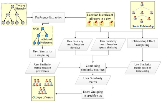
Figure 2.
System architecture for automatic user grouping.
4. Materials and Methods
4.1. User Similarity
This section describes how user similarity is computed based on user preferences, the relationship effect, the user’s free days, and spatial proximity.
4.1.1. Analysing User Preferences
User preferences are extracted according to the categories of his or her visited locations. First, a user location history is projected onto a predefined category hierarchy. As a result, each node receives a value representing the number of visits to a category. This is motivated by the fact that an individual’s preferences are usually made up of multiple interests, such as shopping and visiting historical places, and these interests have different granularities, (e.g., “art and entertainment” → “museum”). Second, The TF-IDF value of each node in the hierarchy is calculated, where a user location history is regarded as a document and categories are considered as terms in the document. Intuitively, if a user likes a particular category, then he/she will visit more locations relating to that category. Furthermore, if a user visits locations within a category that other people use only rarely, it is more likely that this category is of greater interest to this user. For example, the number of visits to restaurants is generally higher than for other categories, such as art galleries in citizen location histories, but this does not imply that food should be ranked as the user’s first interest. However, if a user is found to visit art galleries very frequently, the user may be truly interested in the arts.
Overall, a user’s preference weight (u.wc′) is calculated using Equation (1), where the first part of the equation is the TF value of category c in user u’s location history and the second part denotes the IDF value of the category.
In the above equation, |{u.vi:vi.c = c′}| is user u’s number of visits in category c′, u.V is the total number of the user’s visits and |{uj:c′ ∈ uj.C}| counts the number of users who have visited category c′ among all of the users U in the system. The WCH has several important advantages. It decreases concern about the different data scales of different users, it handles the data sparseness problem and it reduces the computational loads for computing further user similarities (from physical locations to categories). In addition, it enables similarity computation among users who do not have any common physical location histories; in other words, they live in different cities [3,27].
4.1.2. Similarity Based on User Preferences
Similarity computation is achieved via difference methods. In this paper, the cosine distance is used to estimate this value. For each user, a vector is created whose dimension is equal to the number of nodes on the first level of the WCH. The value of each item is the value of the corresponding node. The cosine distance is used to calculate the similarity of two users’ vectors, according to Equation (2):
where are the similarity vectors of two users.
4.1.3. Similarity Based on Relationship
Link prediction is an important research field in data mining with a wide range of scenarios. Many data mining tasks involve the relationships among objects. Link prediction can be used for recommendation systems, social networks, information retrieval, and many other fields [28].
Given that G = ⟨V, E⟩ is a graph of the social network, link prediction involves predicting the probability of the link between node Vi and node Vj. This can be considered as computing the “similarity” between nodes Vi and Vj, according to the network topology. In this paper, Katz’s algorithm (1953) is used for measuring the social relationship effect. The idea of the method is that the existence of more paths between two nodes indicates a greater similarity between the two nodes. The Katz measure is defined as follows [28,29]:
where |pathl u,v| is the number of paths between node u and node v, the length of the path is l, and β is a parameter taking values between zero and one. This parameter is used to control the contribution of a path to the similarity; the longer the path, the less contribution it makes to the similarity. To ensure that the Katz index converges, the value of β must be less than the inverse largest eigenvalue of the adjacency matrix (β < 1/λmax) [30]. The components of the adjacency matrix are defined as follows: if nodes i and j are connected in the network, then aij = 1; otherwise aij = 0.
One strategy for estimating the similarity between two friends is to calculate their common social circles [31]. For this purpose, the similarity between social friends is estimated using the following method:
In Equation (4), specifies a set of users who have a social relationship with user .
Similar check-ins, i.e., check-ins at the same time and location, can also be considered as indicating the similarity of two users who have a social relationship, and can be used to calculate their similarity and social influence using the following method:
In Equation (5), specifies a set of locations that were visited by user . The final relationship similarity therefore is computed as:
4.1.4. Similarity Based on the User’s Free Days
Free time provides citizens with time to spend outdoors and is associated with activities such as shopping, sightseeing, and socializing. These activities contribute to the expansion of relationships and new experiences. Free days vary from person to person, and accepting recommendations is more likely when members of the group share similar free time. This factor, meanwhile, is the key to coordinating group members in the grouping procedure. It can be extracted from location histories in LBSNs. For this purpose, a user-day matrix is computed from the user’s visited locations on a specific day. To normalize the user-day matrix, the TF-IDF is calculated, where a user location history is regarded as a document and the day is considered as a term in the document. The cosine distance is used to calculate the similarity of two users’ vectors.
4.1.5. Spatial Similarity
The geographical proximities of the locations influence the user’s check-in behaviour. Usually, a user prefers to visit locations that are close to his or her residential address or office [4,32,33]. When the distance of the location from a user’s home increases, the user’s probability of visiting that location decreases. The home locations of users are usually not given in the check-in data set due to user privacy concerns. Nevertheless they can be estimated based on the assumption that check-ins are centred around the user’s home location [34,35]. For this purpose, first, a minimum boundary box of the user’s check-in locations is created. Then, this boundary is divided into small non-overlapping regions, and the check-ins are grouped based on those regions. The region with the maximum number of check-ins is considered to be the spatial range within which the user tends to visit venues. The average position of the check-ins inside the region is selected as the centre of the user’s favourite spatial range and an approximation of the user’s home location [35]. After the estimation of the approximate positions that the user has convenient access to, the distances between these positions are estimated. Finally, the users that are spatially closer to each other are considered to be more similar.
4.1.6. Combining Preferences, Relationships, Free Days, and Spatial Similarity
User preferences, social relationships, free days, and spatial proximity are criteria that are combined to compute the final similarity values between each pair of users, as follows:
where the parameters λ, γ and δ control the weights of user preference, relationship, and spatial similarity values, respectively.
4.2. User Grouping for a Given Group Size
For automatic selection of group members in a group recommender system, users are partitioned into groups with a specific group size, based on the similarity of their interests. In this regard, a modified k-medoids method is developed to cluster users into groups with specific sizes. In the proposed method, instead of using linear programming, a Hungarian algorithm is used in assignment phase of the k-medoids algorithm. In order to reduce the running time of the Hungarian algorithm for large data sets, multilevel k-way partitioning is used to divide the data set into the multiple parts. Then, with using parallel computing, the modified k-medoids method is applied for each part.
First, a brief description of the methods used in modified k-medoids algorithm is presented, and then details of the proposed method are described.
4.2.1. Multilevel k-Way Partitioning
The graph partitioning problem is the problem of partitioning the vertices of a graph into p roughly equal partitions so that the number of edges connecting vertices in different partitions is minimized. This approach has attracted great attention in areas such as parallel scientific computing, task scheduling, and VLSI design [36,37].
The k-way partitioning problem is generally solved by recursive bisection. That is, first, a two-way partitioning of V is obtained, and then a two-way partitioning of each resulting partition is determined recursively. After log (k) phases, graph G is partitioned into k partitions. Thus, the problem of performing a k-way partitioning is reduced to performing a sequence of bisections.
The multilevel recursive bisection (MLRB) algorithm has emerged as a highly effective method for computing the k-way partitioning of a graph. The basic structure of a multilevel bisection algorithm is very simple. The graph G is first reduced to a few hundred vertices, a bisection of this much smaller graph is computed, and then this partitioning is projected back to the original graph (with a higher number of vertices) by periodically refining the partitioning. Since the original graph has more degrees of freedom, these refinements decrease the edge cut. A detailed description of this algorithm can be found in [37].
4.2.2. Hungarian Algorithm
The assignment problem is one of the fundamental combinatorial optimization problems in the optimization or operations research branch of mathematics. It consists of finding a maximum weight matching (or minimum weight perfect matching) in a weighted bipartite graph. On the one hand, it is a special case of a more complex problem, such as the generalized assignment problem, the matching problem in graphs or the minimum-cost flow problem. On the other hand, real-world problems, such as the worker assignment problem, can be categorized as this type of problem. In its most general form, the problem can be stated as follows.
Consider a number of agents and tasks. Any agent can be assigned to perform any task, incurring some cost that may vary depending on the agent-task assignment. All of the tasks must be performed by assigning exactly one agent to each task and exactly one task to each agent, in such a way that the total cost of the assignment is minimized.
If the number of agents and tasks are equal and the total cost of the assignment for all of the tasks is equal to the sum of the costs for each agent (or the sum of the costs for each task, which is the same thing in this case), then this is called the linear assignment problem. The Hungarian algorithm is one of a group of algorithms that have been devised to solve the linear assignment problem within a certain time and bounded by a polynomial expression for the number of agents [38,39]. The Hungarian method of finding an optimal assignment is explained in more detail in [38].
4.2.3. k-Medoids Algorithm
In k-medoids methods, a cluster is represented by one of its points. This is an easy solution as it covers any attribute type, and the medoids have been proven to be resistant against outliers because of their insensitivity to peripheral cluster points. When medoids are selected, the clusters are defined as subsets of points close to their respective medoids, and the objective function is defined as the average distance, or another dissimilarity measure, between a point and its medoid [40,41]. The algorithm is as follows:
- Randomly select k data points as medoids.
- Assignment step: Assign each data point to the closest medoids.
- Update step: find new medoids of each cluster to minimize within cluster variance.
- Repeat assignment step and update step until the medoids do not change.
4.2.4. Modified k-Medoids for Grouping People into Groups of a Specific Size
The modified k-medoids method is the same as the standard k-medoids method, except that it guarantees specific cluster sizes. It is also a special case of the constrained k-means method, where cluster sizes are set to be equal or of a specific size. However, instead of using linear programming in the assignment phase, the partitioning is formulated as a pairing problem, which can be solved optimally by a Hungarian algorithm in time O(n3). For large data sets, executing a Hungarian algorithm takes a long time. In order to address this problem, first, multilevel k-way partitioning is used to divide a data set into multiple parts. Then, for each part, the modified k-medoids method is applied to cluster the users and parallel computing is used to reduce the running time.
For ease of expression of the proposed method, it is assumed that the number of users is n and all of the clusters have the same size (k). The process of the modified k-medoids method is similar to k-medoids, however, the assignment phase is different. In this method, instead of selecting the closest medoid, there are n pre-allocated slots (n/k slots per cluster), and data points can be assigned only to these slots (Figure 3). This will force all of the clusters to be of the same size assuming that (, ). Otherwise, there will be (n mod k) clusters of size , and k − (n mod k) clusters of size . To find the assignment that minimizes the mean-square error (MSE), an assignment problem is solved via the Hungarian algorithm. Steps of implementation of the modified k-medoids method are as follows:
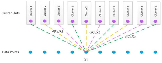
Figure 3.
Minimum distance calculation with balanced clusters (adapted from [26]).
- Data set is divided in multiple parts with k-way partitioning. For each part, the following procedure is repeated.
- The cluster slots are partitioned into clusters with the largest possible even number of slots (it is assumed that all clusters have the same size, if different cluster size is given, cluster slots are divided based on different cluster size.)
- The initial medoids can be select randomly from all data points. (In this study, k-means++ is used to select the initial medoids from all data points.)
- Assignment step: The edge weight is the similarity between the point and the assigned cluster medoid. It is updated according to newly medoids. With using Hungarian algorithm, data points are assigned to cluster slots based on the edge weight.
- Update step: New medoid of each cluster are calculated based on similarity between the points and medoids. The update step is similar to that of the k-medoids method.
- The last two steps are repeated until the medoids do not change.
In contrast to the standard assignment problem with fixed weights, in this study weights are changed dynamically after each k-medoids iteration, according to the newly calculated medoids. Following this, the Hungarian algorithm is performed to obtain the minimal weight pairing. The similarities of the users are stored in an n × n matrix as the correct input format for the Hungarian algorithm. Algorithm 1 provides the pseudocode for the modified k-medoids method.
| Algorithm 1. Modified k-medoids |
Input: data set X, number of member in group Output: partitioning of data set. Partition data set to multi part with k-way partitioning part ← 0 repeat Initialize medoid locations C0 with k-means++ t ← 0 repeat Assignment step: Calculate edge weights. Solve an Assignment problem. Update step: Calculate new medoid locations Ct+1 t ← t + 1 Until medoid locations do not change. Until all parts are clustering |
4.3. Experimental Evaluation
In this section, first the settings of the experiments, including the data set, baseline approaches, and the evaluation method, are described. Results regarding both the effectiveness and the efficiency of the proposed system are presented and followed by a discussion.
Experimental Settings
Data sets. The two largest cities in the USA, New York City (NYC) and Los Angeles (LA), are considered in this study. Data sets from these cities, including the tips generated by users, are extracted from Foursquare [27]. Four data sets from the above-mentioned cities have been selected as follows. (1) Users whose home city is LA and who are visitors to places in LA, (2) users from New Jersey who visit LA, (3) users from New York visiting places within their city, and (4) users from New Jersey who are visiting New York. Statistics of experimental data sets are shown in Table 1. These data sets were collected during a period of 25 months from 1 February 2009 to 30 July 2011.

Table 1.
Statistics of experimental data sets.
Foursquare has blocked the API for crawling a user’s check-in data due to privacy concerns. However, the tips left by users are available for download. The proposed method could be more effective if check-in data was used, although it seems sensible to use tips as there are some associated advantages, such as the fact that they express a user’s real interests. Sometimes, people check in at a venue without visiting the venue for any purpose. However, leaving a tip in connection with a venue usually means that the user has engaged in some essential activities, such as dining or shopping at the venue [27].
The following information is extracted: (1) user profile information, including the user ID, name, and home city, (2) the user’s social relationships, including the user IDs of two-sided connections, (3) venue profile information, consisting of a venue’s ID, name, address, GPS coordinates, and categories, and (4) user location histories, represented by all of the tips a user has left in the system. Each tip includes a venue ID, comments, and a timestamp. From the data set, the users who have over seven tips in a city are chosen as candidate query users.
Evaluation methods. For the evaluation of clustering solutions, validity indices are normally used. There are two types of validity indices: external indices and internal indices [42]. An external index is a measure of the agreement between two partitions where the first partition is the a priori known clustering structure, and the second results from the clustering procedure [43]. Internal indices are used to measure the quality of a clustering structure without external information. For internal indices, the results are evaluated using quantities and inherent features of the data set. In this paper, the ground truth labels are not known, therefore internal indices must be used. There are several internal indices for clustering evaluation.
As mentioned previously, users will be partitioned into groups of a specific size, in a process that differs from general clustering. It is mandatory that users are partitioned with similar preferences. Therefore, the intra-cluster distances are important for the evaluation of clustering, while the inter-cluster distances are not significant. The mean intra-cluster distance and the silhouette index are used for evaluating the proposed method. In addition, the three clustering methods of spectral clustering, k-medoids, and k-way partitioning are used for grouping users. The outcomes from these methods and from the proposed approach are compared and discussed.
Mean intra-cluster distance. In each cluster, the intra-cluster distances between points should be as small as possible. The mean intra-cluster distance for all of the clusters is an efficient index for evaluating the results of clustering.
Silhouette index. The silhouette refers to a method of interpretation and validation with respect to consistency within clusters of data. The silhouette value is a measure of how similar an object is to its own cluster (cohesion) compared to other clusters (separation). The silhouette is based on the mean score for every point in the data set (Equation (8)). Each point’s individual score is based on the difference between the average distance of that point to other points in its cluster and the minimum average distance between that point and the other points of other clusters. This difference is then divided by a normalization term, which is the average with the larger value,
where, N is the number of points in the data set, and
If is a point in cluster p, then where is the average distance between point and every point of cluster q. On the other hand, is the average distance between point and every other point of cluster p. The score range is between −1 and 1, indicating that as clustering improves, then the score will approach a value of 1 [44].
Parameter selection. The terms λ, γ and δ are parameters that stand for the weights of the user preference, relationship and spatial similarity values respectively. Subsequently, these parameters determine the weight of users’ free day similarities. Due to the fact that the attractiveness of friendship with new individuals, visiting new places and the possibility to change free days may not be similar for all individuals, the λ, γ and δ parameters can vary from case to case. In this study, the values of these parameters are selected by a parameter space search with silhouette criteria, according to which λ, γ and δ parameter values are set to 0.3, 0.2, and 0.25, respectively.
5. Results and Discussion
For convenience, the group sizes are assumed to be equal with each group having six members. The proposed method is applied to the four selected data sets. For each data set, user preferences, social relationships, spatial proximity, users’ free days, and final similarities, (where the latter is a combination of the first four factors with estimated weights), are considered separately for clustering. The mean intra-cluster distance and silhouette index values are calculated for the evaluation of clustering in each data set. Results of the evaluation for database #1 are shown in Table 2.
Table 2.
Results of evaluation methods for automatic user grouping (database #1).
The silhouette index range is between −1 and 1, where a score that is closer to 1 indicates better clustering. As can be seen from Table 2, the silhouette score is near to zero because users are grouped in groups of specific size; this issue is different from the case of general clustering. Users with similar preferences are mandatorily partitioned where large clusters are forced to break up into clusters of a specific size. This causes similar individuals to be defined as different clusters, and consequently causes the distance to the nearest cluster to be reduced. In other words, the separations of the clusters are reduced, causing the silhouette score to be near zero. The positive silhouette score, however, indicates that the separation of the clusters is greater than the cohesion of the clusters over the majority of the points.
Similarity of clusters, as represented by low variances, is of greater importance than the distance between clusters, which decreases when the number of cluster members is reduced. For the mean intra-cluster distance, a lower value represents more cohesion within clusters. For example, in Table 2, the mean intra-cluster distance when only user preference similarity (λ = 1, γ = 0, δ = 0) is considered for grouping the users, is estimated at 0.072. From Table 2, for the selected parameters (λ = 0.3, γ = 0.2, δ = 0.25), the mean intra-cluster distance is 0.192. In the next phase, and in order to better interpret the values shown in Table 2, the mean intra-cluster distances of the other factors are estimated separately for previously defined clusters. These values are shown in Table 3 for database #1. In Table 3, column 1 indicates that only the user preference similarity is considered for partitioning users, and the mean intra-cluster distances of social relationships, spatial proximity, and free days (temporal distance) are measured for the determined groups. The other columns of Table 3 can be interpreted in a similar way.
Table 3.
The mean intra-cluster distances of user preference, spatial proximity, social relationships, and free days for database #1.
The last column of Table 3 implies that by taking into account the user preferences, social relationships, users’ free days, and spatial proximity, the mean intra-cluster distance is estimated at 0.191. After grouping the users, the mean intra-cluster distances of these factors are estimated at 0.170, 0.338, 0.242, and 0.112, respectively. According to Table 3, grouping users with one criterion decreases the mean intra-cluster distance value for that criterion, but this value then increases for the other factors. Table 3 shows that the value of the mean intra-cluster distance in social relationships is comparatively high, due to the lack of relationships among all of the users and a relatively small similarity value.
In order to evaluate the efficiency of the proposed method, the outcomes of this study are compared with other clustering algorithms. These algorithms, i.e., k-medoids and spectral methods, are two common clustering approaches that are applied to grouping people. In addition, multilevel k-way partitioning is used in this assessment because it creates a balanced partition. In these methods, the number of clusters must be specified. In this study, it is assumed that the group size is fixed, each group having six members. With this assumption, the number of desired clusters is achieved by dividing the number of users by the size of each cluster. The results show that the cluster sizes in the k-medoids and spectral clustering methods were not equal, so that either one point or a huge proportion of the data may be allocated to a single cluster, while the multilevel k-way partitioning creates balanced cluster sizes. In k-medoids, the number of clusters is less than the specified number of clusters; in some cases, some clusters do not even contain any points. In spectral clustering and multilevel k-way partitioning, the number of clusters is equal to the specified number of clusters.
In Table 4, the average of the cluster size distribution (per cent) in the proposed method, multilevel k-way partitioning, k-medoids, and spectral clustering methods are compared. As can be observed, in the k-medoids and spectral clustering methods, a high percentage of the clusters do not share the same specified size, while in the proposed method and in multilevel k-way partitioning a high percentage of the clusters are of equal size.
Table 4.
The average of Cluster size distribution (per cent) resulting from the proposed and three existing clustering approaches.
The mean intra-cluster distances of the four different approaches for the four data sets are compared in Table 5. As the number of clusters with small sizes is outnumbered in k-medoids and spectral clustering, the mean intra-cluster distances of the methods are small. In order to compare the outcomes of the proposed method with those of k-medoids and spectral clustering, clusters with a size of less than four are removed in the mean intra-cluster distance calculation. The mean intra-cluster distance that is calculated by the proposed method is fairly small. According to Table 5, although multilevel k-way partitioning divided users into balanced cluster sizes, the mean intra-cluster distance in this method is higher than in the proposed method. Furthermore, in the multilevel k-way partitioning method, cluster sizes cannot change based on a predefined cluster size.
Table 5.
The mean intra-cluster distance of the proposed method and three clustering approaches for the four data sets.
6. Conclusions
In a spatial group recommender system, the system recommends a place to a group of users. In this study, an automatic method for identifying groups of users with similar preferences, spatial proximity, free days, and social relationships has been proposed. Corresponding data sets for the parameters mentioned were obtained from the location histories and user profiles. Then, a modified k-medoids clustering algorithm was developed, which guarantees equal clusters or clusters of a specific size. The proposed method was evaluated using further experiments based on four data sets that were collected from Foursquare. The mean intra-cluster distance and the silhouette index were used for evaluating the proposed method. In addition, the three clustering methods of spectral clustering, k-medoids, and k-way partitioning were used for grouping users. The results of these methods and the results of the proposed approach were compared. The results showed that the proposed method can efficiently divide users into groups with a given group size. The mean intra-cluster distance for the proposed method is almost identical to that for the spectral clustering and k-medoids methods. However, the proposed method meets the objective of partitioning users into groups of a specific size. Although multilevel k-way partitioning created balanced cluster sizes, the proposed method has a comparatively lower mean intra-cluster distance. The proposed method is capable of partitioning users into clusters with specific predetermined sizes.
Foursquare is one of the most popular LBSNs worldwide, so data sets of this network have been used as an example and are representative of other LBSNs. So, results of the proposed approach for user grouping can be generalized to other LBSNs. Also, the proposed user grouping method can be used in other fields that needs user grouping, such as citizen science. In this study, location category is used for the determination of user preferences, and physical locations of users are ignored. Only the visited venue locations are used in order to calculate the spatial proximity of users. For future studies, inferring the spatial preferences of users by considering the physical locations and including the temporal influences and group sizes on the clustering results are aspects that are recommended for further investigation. Moreover, it is worth noting that in the context of the spatial group recommender system, a procedure for suggesting places according to preferences of the group members could be developed. Because of a lack of information about the uncertainty, reliability of the existing data sets has not been considered in this research, and it has been assumed that users’ checks in at a place are correct and reflect their true preferences. Consideration of uncertainty and bias effects in crowdsourcing data is an important topic [45,46,47] and can be considered in future studies.
Author Contributions
Elahe Khazaei and Abbas Alimohammadi conceived and designed the experiments; Elahe Khazaei carried out model development, verification the models, and drafted the original version of the manuscript. Abbas Alimohammadi helped to revise the paper.
Conflicts of Interest
The authors declare no conflict of interest.
References
- Bao, J.; Zheng, Y.; Wilkie, D.; Mokbel, M. Recommendations in location-based social networks: A survey. Geoinformatica 2015, 19, 525–565. [Google Scholar] [CrossRef]
- Abbasi, O.; Alesheikh, A.; Sharif, M. Ranking the City: The Role of Location-Based Social Media Check-Ins in Collective Human Mobility Prediction. ISPRS Int. J. Geo-Inf. 2017, 6, 136. [Google Scholar] [CrossRef]
- Wang, H.; Li, G.; Feng, J. Group-Based Personalized Location Recommendation on Social Networks. In APWeb; Chen, L., Jia, Y., Sellis, T., Liu, G., Eds.; Lecture Notes in Computer Science; Springer International Publishing: Cham, Switzerland, 2014; Volume 8709, pp. 68–80. ISBN 978-3-319-11115-5. [Google Scholar]
- Wang, H.; Terrovitis, M.; Mamoulis, N. Location recommendation in location-based social networks using user check-in data. In Proceedings of the 21st ACM SIGSPATIAL International Conference on Advances in Geographic Information Systems - SIGSPATIAL’13; ACM Press: New York, New York, USA, 2013; pp. 364–373. [Google Scholar]
- Guo, J.; Zhu, Y.; Li, A.; Wang, Q.; Han, W. A Social Influence Approach for Group User Modeling in Group Recommendation Systems. IEEE Intell. Syst. 2016, 31, 40–48. [Google Scholar] [CrossRef]
- Butler, C.T.L.; Rothstein, A. On Conflict and Consensus: A Handbook on Formal Consensus Decisionmaking, 3rd ed.; Food Not Bombs: Santa Cruz, CA, USA, 2007. [Google Scholar]
- Kompan, M.; Bielikova, M. Group Recommendations: Survey and Perspectives. Comput. Inform. 2014, 33, 446–476. [Google Scholar]
- Purushotham, S.; Kuo, C.-C.J.; Shahabdeen, J.; Nachman, L. Collaborative Group-activity Recommendation in Location-based Social Networks. In Proceedings of the 3rd ACM SIGSPATIAL International Workshop on Crowdsourced and Volunteered Geographic Information; GeoCrowd’14; ACM: New York, NY, USA, 2014; pp. 8–15. [Google Scholar]
- Ludovico, B.; Salvatore, C.; Satta, M. Groups identification and individual recommendations in group recommendation algorithms. Proceedings of Workshop on the Practical Use of Recommender Systems, Algorithms and Technologies (PRSAT 2010), Barcelona, Spain, 30 September 2010. [Google Scholar]
- Chang, X.; Nie, F.; Ma, Z.; Yang, Y. Balanced k-Means and Min-Cut Clustering. arXiv preprint 2014. [Google Scholar]
- Boratto, L.; Carta, S. State-of-the-Art in Group Recommendation and New Approaches for Automatic Identification of Groups. In Information Retrieval and Mining in Distributed Environments; Soro, A., Vargiu, E., Armano, G., Paddeu, G., Eds.; Studies in Computational Intelligence; Springer Berlin Heidelberg: Berlin/Heidelberg, Germany, 2011; pp. 1–20. [Google Scholar]
- Kim, J.K.; Kim, H.K.; Oh, H.Y.; Ryu, Y.U. A group recommendation system for online communities. Int. J. Inf. Manage. 2010, 30, 212–219. [Google Scholar] [CrossRef]
- Pizzutilo, S.; De Carolis, B.; Cozzolongo, G.; Ambruoso, F. Group modeling in a public space: Methods, techniques, experiences. In Proceedings of the 5th WSEAS International Conference on Applied Informatics and Communications, Stevens Point, WI, USA, 15–17 September 2005; pp. 175–180. [Google Scholar]
- Smyth, B.; Balfe, E. Anonymous personalization in collaborative web search. Inf. Retr. Boston. 2006, 9, 165–190. [Google Scholar] [CrossRef]
- O’Connor, M.; Cosley, D.; Konstan, J.A.; Riedl, J. PolyLens: A recommender system for groups of users. In ECSCW 2001: Proceedings of the Seventh European Conference on Computer Supported Cooperative Work 16–20 September 2001, Bonn, Germany; Springer: Dordrecht, The Netherlands, 2001; pp. 199–218. [Google Scholar]
- Ardissono, L.; Goy, A.; Petrone, G.; Segnan, M.; Torasso, P. Intrigue: Personalized recommendation of tourist attractions for desktop and hand held devices. Appl. Artif. Intell. 2003, 17, 687–714. [Google Scholar] [CrossRef]
- McCarthy, J.F. Pocket Restaurant Finder: A situated recommender systems for groups. In Proceedings of the Workshop on Mobile Ad-Hoc Communication at the 2002 ACM Conference on Human Factors in Computer Systems, Minneapolis, MN, USA, 20–25 April 2002; pp. 1–10. [Google Scholar]
- Lieberman, H.; Van Dyke, N.W.; Vivacqua, A.S. Let’s Browse: A Collaborative Web Browsing Agent. In Proceedings of the 4th International Conference on Intelligent User Interfaces; IUI ’99; ACM: New York, NY, USA, 1999; pp. 65–68. [Google Scholar]
- Crossen, A.; Budzik, J.; Hammond, K. J. Flytrap. In Proceedings of the 7th International Conference on Intelligent User Interfaces - IUI ’02; ACM Press: New York, NY, USA, 2002; p. 184. [Google Scholar]
- Newman, M.E.J.; Girvan, M. Finding and evaluating community structure in networks. Phys. Rev. E 2004, 69, 26113. [Google Scholar] [CrossRef] [PubMed]
- Newman, M.E.J. Analysis of weighted networks. Phys. Rev. 2004, 70. [Google Scholar] [CrossRef] [PubMed]
- Blondel, V.D.; Guillaume, J.-L.; Lambiotte, R.; Lefebvre, E. Fast unfolding of communities in large networks. J. Stat. Mech. Theory Exp. 2008, 2008, P10008. [Google Scholar] [CrossRef]
- Cantador, I.; Castells, P. Extracting multilayered Communities of Interest from semantic user profiles: Application to group modeling and hybrid recommendations. Comput. Human Behav. 2011, 27, 1321–1336. [Google Scholar] [CrossRef]
- Li, Y.-M.; Chou, C.-L.; Lin, L.-F. A social recommender mechanism for location-based group commerce. Inf. Sci. 2014, 274, 125–142. [Google Scholar] [CrossRef]
- Ganganath, N.; Cheng, C.-T.; Tse, C.K. Data Clustering with Cluster Size Constraints Using a Modified K-Means Algorithm. In Proceedings of the 2014 International Conference on Cyber-Enabled Distributed Computing and Knowledge Discovery, Shanghai, China, 13–15 October 2014; pp. 158–161. [Google Scholar]
- Malinen, M. I.; Fränti, P. Balanced K-Means for Clustering. In Structural, Syntactic, and Statistical Pattern Recognition; Springer: Berlin/Heidelberg, Germany, 2014; pp. 32–41. [Google Scholar]
- Bao, J.; Zheng, Y.; Mokbel, M. F. Location-based and preference-aware recommendation using sparse geo-social networking data. In Proceedings of the 20th International Conference on Advances in Geographic Information Systems - SIGSPATIAL’12; ACM Press: New York, NY, USA, 2012; p. 199. [Google Scholar]
- Dong, L.; Li, Y.; Yin, H.; Le, H.; Rui, M.; Dong, L.; Li, Y.; Yin, H.; Le, H.; Rui, M. The Algorithm of Link Prediction on Social Network. Math. Probl. Eng. 2013, 2013, 1–7. [Google Scholar] [CrossRef]
- Liben-Nowell, D.; Kleinberg, J. The Link Prediction Problem for Social Networks. Proc. Twelfth Annu. ACM Int. Conf. Inf. Knowl. Manag. 2003, 556–559. [Google Scholar] [CrossRef]
- Wu, J.; Hou, Y.; Jiao, Y.; Li, Y.; Li, X.; Jiao, L. Density shrinking algorithm for community detection with path based similarity. Phys. A Stat. Mech. Appl. 2015, 433, 218–228. [Google Scholar] [CrossRef]
- Cheng, C.; Yang, H.; King, I.; Lyu, M.R. Fused matrix factorization with geographical and social influence in location-based social networks. Proceedings of Twenty-Sixth AAAI Conference on Artificial Intelligence, Toronto, ON, Canada, 22–26 July 2012; pp. 17–23. [Google Scholar]
- Ye, M.; Yin, P.; Lee, W.-C.; Lee, D.-L. Exploiting geographical influence for collaborative point-of-interest recommendation. In Proceedings of the 34th International ACM SIGIR Conference on Research and Development in Information - SIGIR’11; ACM Press: New York, NY, USA, 2011; p. 325. [Google Scholar]
- Hu, L.; Sun, A.; Liu, Y. Your Neighbors Affect Your Ratings: On Geographical Neighborhood Influence to Rating Prediction. In Proceedings of the 37th International ACM SIGIR Conference on Research & Development in Information Retrieval; SIGIR ’14; ACM: New York, NY, USA, 2014; pp. 345–354. [Google Scholar]
- Rahimi, S.M.; Wang, X. Location Recommendation Based on Periodicity of Human Activities and Location Categories. In Advances in Knowledge Discovery and Data Mining; Springer: Berlin/ Heidelberg, Germany, 2013; pp. 377–389. [Google Scholar]
- Zhou, D.; Rahimi, S.M.; Wang, X. Similarity-based probabilistic category-based location recommendation utilizing temporal and geographical influence. Int. J. Data Sci. Anal. 2016, 1, 111–121. [Google Scholar] [CrossRef]
- Heith, M. T.; Raghavan, P. A Cartesian parallel nested dissection algorithm. SIAM J. Matrix Anal. Appl. 1992, 19, 235–253. [Google Scholar] [CrossRef]
- Karypis, G.; Kumar, V. Multilevelk-way Partitioning Scheme for Irregular Graphs. J. Parallel Distrib. Comput. 1998, 48, 96–129. [Google Scholar] [CrossRef]
- Kuhn, H.W. The Hungarian method for the assignment problem. Nav. Res. Logist. Q. 1955, 2, 83–97. [Google Scholar] [CrossRef]
- Kuhn, H.W. Variants of the hungarian method for assignment problems. Nav. Res. Logist. Q. 1956, 3, 253–258. [Google Scholar] [CrossRef]
- Berkhin, P. Survey of Clustering Data Mining Techniques; Technical Report; Accrue Software Inc.: San Jose, CA, USA, 2002. [Google Scholar]
- Velmurugan, T.; Santhanam, T. Computational Complexity between K-Means and K-Medoids Clustering Algorithms for Normal and Uniform Distributions of Data Points. J. Comput. Sci. 2010, 6, 363–368. [Google Scholar] [CrossRef]
- Wang, K.; Wang, B.; Peng, L. CVAP: Validation for Cluster Analyses. Data Sci. J. 2009, 8, 88–93. [Google Scholar] [CrossRef]
- Dudoit, S.; Fridlyand, J. A prediction-based resampling method for estimating the number of clusters in a dataset. Genome Biol. 2002, 3, RESEARCH0036. [Google Scholar] [CrossRef]
- Baarsch, J.; Celebi, M.E. Investigation of internal validity measures for K-means clustering. In Proceedings of the International Multiconference of Engineers and Computer Scientists, Hong Kong, China, 14–16 March 2012; pp. 14–16. [Google Scholar]
- Quattrone, G.; Capra, L.; De Meo, P. There’s No Such Thing as the Perfect Map: Quantifying Bias in Spatial Crowd-sourcing Datasets. In Proceedings of the 18th ACM Conference on Computer Supported Cooperative Work & Social Computing, Vancouver, BC, Canada, 14–18 March 2015; pp. 1021–1032. [Google Scholar]
- Zhang, J.; Sheng, V.S.; Li, Q.; Wu, J.; Wu, X. Consensus algorithms for biased labeling in crowdsourcing. Inf. Sci. 2017, 382–383, 254–273. [Google Scholar] [CrossRef]
- Chakraborty, A.; Messias, J.; Benevenuto, F.; Ghosh, S.; Ganguly, N.; Gummadi, K.P. Who Makes Trends? Understanding Demographic Biases in Crowdsourced Recommendations. In Proceedings of the 11th AAAI International Conference on Web and Social Media (ICWSM 2017), Montreal, CA, USA, 15–18 May 2017. [Google Scholar]
© 2018 by the authors. Licensee MDPI, Basel, Switzerland. This article is an open access article distributed under the terms and conditions of the Creative Commons Attribution (CC BY) license (http://creativecommons.org/licenses/by/4.0/).