Approach to Accelerating Dissolved Vector Buffer Generation in Distributed In-Memory Cluster Architecture

Abstract

The buffer generation algorithm is a fundamental function in GIS, identifying areas of a given distance surrounding geographic features. Past research largely focused on buffer generation algorithms generated in a stand-alone environment. Moreover, dissolved buffer generation is data- and computing-intensive. In this scenario, the improvement in the stand-alone environment is limited when considering large-scale mass vector data. Nevertheless, recent parallel dissolved vector buffer algorithms suffer from scalability problems, leaving room for further optimization. At present, the prevailing in-memory cluster-computing framework—Spark—provides promising efficiency for computing-intensive analysis; however, it has seldom been researched for buffer analysis. On this basis, we propose a cluster-computing-oriented parallel dissolved vector buffer generating algorithm, called the HPBM, that contains a Hilbert-space-filling-curve-based data partition method, a data skew and cross-boundary objects processing strategy, and a depth-given tree-like merging method. Experiments are conducted in both stand-alone and cluster environments using real-world vector data that include points and roads. Compared with some existing parallel buffer algorithms, as well as various popular GIS software, the HPBM achieves a performance gain of more than 50%.

1. Introduction

A vector buffer in GIS (geographic information systems) is defined as the zone around a geometric geographic feature, measured in units of distance or time [1]. Vector buffer analysis is a fundamental function in the GIS domain for proximity analysis, area range computation, hybrid overlay analysis, spatial data query/filter and so on. It determines the neighborhood degree in GIS [2].

Buffer generation is the key to vector buffer analysis. Several methods for solving the generation problem of vector buffers have been proposed. According to whether or not the buffer zones of each feature are merged, the problem can be classified into two types: buffering with dissolved boundaries and buffering with intact boundaries, which are frequently used in modern GIS systems http://pro.arcgis.com/en/pro-app/tool-reference/analysis/buffer.htm http://docs.qgis.org/2.18/en/docs/gentle_gis_introduction/vector_spatial_analysis_buffers.html (Figure 1).

Figure 1. Two types of vector buffer.

Vector buffer analysis itself is computation-intensive and time-consuming. Moreover, the rapid growth of available large-scale geographic data has increased the complexity and difficulty of buffer analysis. Many strategies for optimizing the problem have been proposed. Most of them concentrate on accelerating the buffer zone construction [3,4,5,6]. Typically, the edge constraint triangulation method [7] and the buffer equation approximation strategy are widely accepted [8]. Also, many algorithms have been designed to address buffer zone dissolving [9,10,11]. This is because the dissolved type of buffer, compared with the undissolved one, is applied more frequently. At present, the recognized efficient algorithms—including Vatti’s algorithm [12] and the Greiner–Hormann algorithm [13]—can be used to process an arbitrary self-intersection with polygon dissolving.

Although excellent performances have been achieved, these optimized methods are carried out simply on the basis of the stand-alone serial approach. Therefore, their computational optimization ability is limited if addressing large-scale mass geodata. Parallel computing and distributed computing are ways of exploiting parallelism in computing to achieve higher performances. In this article, we regard distributed computing as a special form of parallel computing.

Thus, several parallel strategies have been put forward to solve those bottleneck problems. The first strategy is based on the MPI (message passing interface) protocol, which supports the parallel execution of buffer analysis algorithms on HPC (high-performance computing) cluster computers [14,15,16,17] but suffers from weak extensibility when faced with the big spatial data scenarios. The second strategy comes from the distributed high-performance computing framework for big data, MapReduce and Spark, which have recently gained much attention and popularity in the field of geoanalysis. Despite the fact that they do not natively support spatial data and spatial analysis, abundant expansion frameworks have gradually been created and applied in spatial computing. These frameworks include Hadoop-GIS [18], SpatialHadoop [19], SpatialSpark [20], GeoSpark [21], LocationSpark [22], and Simba [23]. They provide a variety of basic spatial functions, for example, spatial index construction, spatial range query, and k-nearest neighbors query (k-NN). Unfortunately, these extended frameworks do not yet support buffer processing. However, we observe that Spark has already been used in spatial overlay analysis [24] and spatial multi-way join calculation [25], suggesting its potential application to buffer analysis.

Thus, in this paper, we propose a parallel vector buffer analysis framework that takes advantage of the in-memory architecture of the Spark platform and further improves its performance by utilizing a space-filling-curve coding technology with a sampling-based partitioning strategy and a depth-given tree-like merging method.

The main contributions of this paper are as follows:

• Space-filling curves are studied and proved to be effective in preserving spatial neighborhood properties and avoiding data skew under the Spark platform. The corresponding methods are designed.
• A number of methods are put forward by using a Hilbert spatial-filling curve partition method to acquire the aggregation attribute, avoid data skew, address the boundary intersection, decompose data partitions with a load balance, and perform polygon merging in a more effective, tree-like way.
• Using a real dataset, we show the superior performances of different strategies and verify the effectiveness of this method.

This paper is organized as follows: Section 2 highlights related work and literature. Section 3 describes the practical problems of buffer analysis in a parallel environment. Section 4 focuses on the optimization methods. Then, the computational cost comparison between the proposed HPBM and other algorithms is analyzed in Section 5. The experimental results are presented and discussed in Section 6.

2. Related Work

The calculation of buffers is an important operation of geographic information systems. The dissolved vector buffer generation is even more significant in research and engineering applications. According to the computational architecture adopted, studies on this problem can be regarded as offering one of two technological solutions: calculation of the buffer zones in a serial computing model and the construction of massive buffer zones via a parallel computing framework.

The first mainly focuses on the outline generation of a buffer zone for each geometric feature and self-intersection tackled among simple buffer zones. Dong [3] proposed a method that adopts the rotation transform point formula and recursion approach to improve the vector buffer generation process for double parallel lines and circular arcs. The circular correction of sharp angles is also improved. Ren [26] proposed a method based on the Douglas-Peucker algorithm that removes the non-characteristic points from the original geometry and keeps the characteristic points, thus reducing the computing cost of buffer zone generation. LI [27] introduced a method for creating buffer zones based on the dilation algorithm, which first converts the geographic entities into the raster type and then carries out 4-accessibility dilation and 8-accessibility dilation alternatively. Wang [5] introduced buffer generation methods based on the vector boundary tracing strategy, which improved the efficiency of point-arc distance calculation. Zalik et al. [28] proposed a method based on a sweep-line approach to construct the geometric outlines of a given set of line segments. The method first creates outlines of the basic geometric buffers (BGBs) and then identifies the intersection points between the outlines of the BGBs. Finally the closed paths of edges are constructed, and the spatial relationships among the closed paths are determined. Based on Zalik’s method, Sumeet Bhatia [29] presented an extended algorithm for constructing geometric buffers for vector feature layers and dissolving those buffers using a sweep-line approach and vector algebra. Emre [30] proposed a buffer zone computation algorithm for the rendering of corridors in GIS applications.

The aforementioned algorithms require complex computations to utilize geometric algorithms and identify spatial relationships. Moreover, subject to the limitation of the serial computing architecture, the computing time is more difficult to decrease when applied to the massive data scenario.

With the development of computer hardware technology, there has been a rapid expansion in the number of available processing cores (consider, e.g., multicore machines, server clusters and cloud computing), thus making high-performance computing an increasingly important issue when analyzing, processing and visualizing massive amounts of geospatial data [31]. Parallelization is an effective way to improve the performance of buffer computation and is becoming more common in routine applications due to decreasing hardware costs and the availability of open source software programs that support this architecture. These methods can generally be regarded as types of parallel computing since many calculations or processes are carried out simultaneously. According to the computing architecture, early parallel buffer method can be roughly classified into one of three categories.

The first is computing-grid-oriented methods. The grid-oriented methods are based on grid computing https://en.wikipedia.org/wiki/Grid_computing, which is one kind of parallel computing method. Yao [14] introduced a parallel algorithm for buffer analysis based on the computing grid platform, which builds distributed tasks according to different map layers and geographic areas. The algorithm has been tested in an urban road planning application, but the method may lead to sub-tasks being unbalanced when the data volumes in different grids vary greatly. Pang [15] proposed another solution for buffer analysis via a service-oriented distributed grid environment. Pang’s method takes a master-slave architecture and distributes N entities to M slave computing nodes, each of which can process $N/M$ entities. The master node combines the results from all slave nodes and works out the final buffer zones.

The second category is parallel-cluster-oriented methods. In this computing environment, a computer cluster can be viewed as a single system. To be more specific, the parallel buffer methods depend on the MPI, which is one of the most popular parallel computing methods used today. Huang [16] presented an integrated solution in a parallel cluster to accelerate the buffer generation; this solution consists of a point-based partition strategy and a binary-union-tree-based buffer zone dissolving method. The solution was applied to a two-node self-build cluster with a dataset containing 200,000 features. Fan [17] proposed a parallel buffer algorithm based on area merging and vertex partitioning to improve the performances of buffer analyses when processing large datasets. Fan implemented the algorithm in the MPI programming model, which is the mainstream architecture in high-performance computing. Fan also took the vertex-number-oriented parallel task partition strategy and a tree-like area merging approach and found this method to be effective in improving the performance of dissolved buffer construction via and inter-process parallel strategy. However, Fan’s experiments were conducted only on a stand-alone computer with 4 MPI processes and claimed the extensive processing to be complex. Wang [32] introduced a parallel buffer generation algorithm, which was based on the arc partition strategy instead of the point partition strategy used in previous works, to ensure better load balance performance. The proposed method was tested on the GRASS GIS with MPI parallel programming model for a 4-node cluster.

The third category is the prevailing architecture for big data processing. In recent years, Hadoop, Spark, and other big data processing frameworks have greatly improved the efficiency of data processing. Research has shown that it is possible to carry out large-scale spatial data calculations over these architectures. Based on Hadoop, Fan introduced solutions for GIS analysis including the buffer algorithm [33], which runs on at most five nodes, achieving higher performance in the case of a large data volume compared to that in the small data volume scenario. Here, the line vector objects are split into smaller objects according to the grid border. Nevertheless, this method experiences problems, including data skew and task imbalance. We also note that one project named Magellan [34] has been developed to support buffer-included analysis based on Spark. At the same time, some other spatial analyses are also supported by Spark. In overlay analysis [24], the utilization of a uniform grid partition method accelerates the overlay process. Likewise, a grid partition strategy has also been applied in spatial join processing [25]. As mentioned in these two articles, the Spark environment provides positive results. Thus, further research based on this framework is needed.

As a computing architecture, the significant performance gain of Apache Spark has been demonstrated [35]. Apache Spark is an open-source cluster-computing framework that provides an interface for programming entire clusters with implicit data parallelism and fault tolerance.

Regarding the current buffer methods, they are utilized in three different categories of computing environment. The first category of methods has deteriorated performances when addressing large-scale vector data due to geographically unbalanced data. Regarding the methods of the second category, they not only take the spatial aggregation attribution into consideration but are also confined by the complexity of programming when the number of processes increases. Methods based on the prevailing Hadoop architecture either lack partition strategies for spatial partitions or have limited performances when applied to large-scale data. Moreover, there is a lack of Spark-related research.

Based on this sequence, we have developed HPBM—a high-performance vector buffer algorithm based on Spark. The goal of our method is to achieve a scalable, efficient and adaptive vector buffer algorithm for spatially unbalanced massive vector data. Our method provides a Hilbert-curve-based adaptive data partition to alleviate the complexity brought by spatially unbalanced data. By using a depth-given tree-like merger strategy, the intermediate results in parallel buffer generation are reduced to achieve higher performance. Moreover, spatial buffer analysis is intrinsically complex, as it often relies on effective access methods to alleviate the high cost of geometric computations. Thus, the Spark computing infrastructure is chosen for this computation-intensive analysis.

3. Problem Definition and Description

From recent studies, we find that a cluster computing paradigm over distributed shared memory for big data processing, such as Spark, is also a promising solution for large-scale spatial analysis. However, detailed methods for data partitioning, task dispatching and result merging are needed.

Thus, the problem could be described as follows: Consider geospatial dataset D, which contains n objects and is expressed as $D=\left\{d_i|i=1,2,\dots ,N\right\}$, where N is the total number of objects in D and $d_i$ is the ith object of D. The goal is to compute the buffer zones (in the Spark environment) around each object in D and dissolve them into one (or several) integral polygons, denoted as G.

The symbols used in this article are presented in Table 1 below.

Table 1. Symbols used in this study.

Symbol	Description
N	Total number of objects of input data
V	Total number of vertices of input data
D	Single data block
d	Single object
v	Single vertex
p	Number of data blocks
G	Buffer and dissolved result in one data block

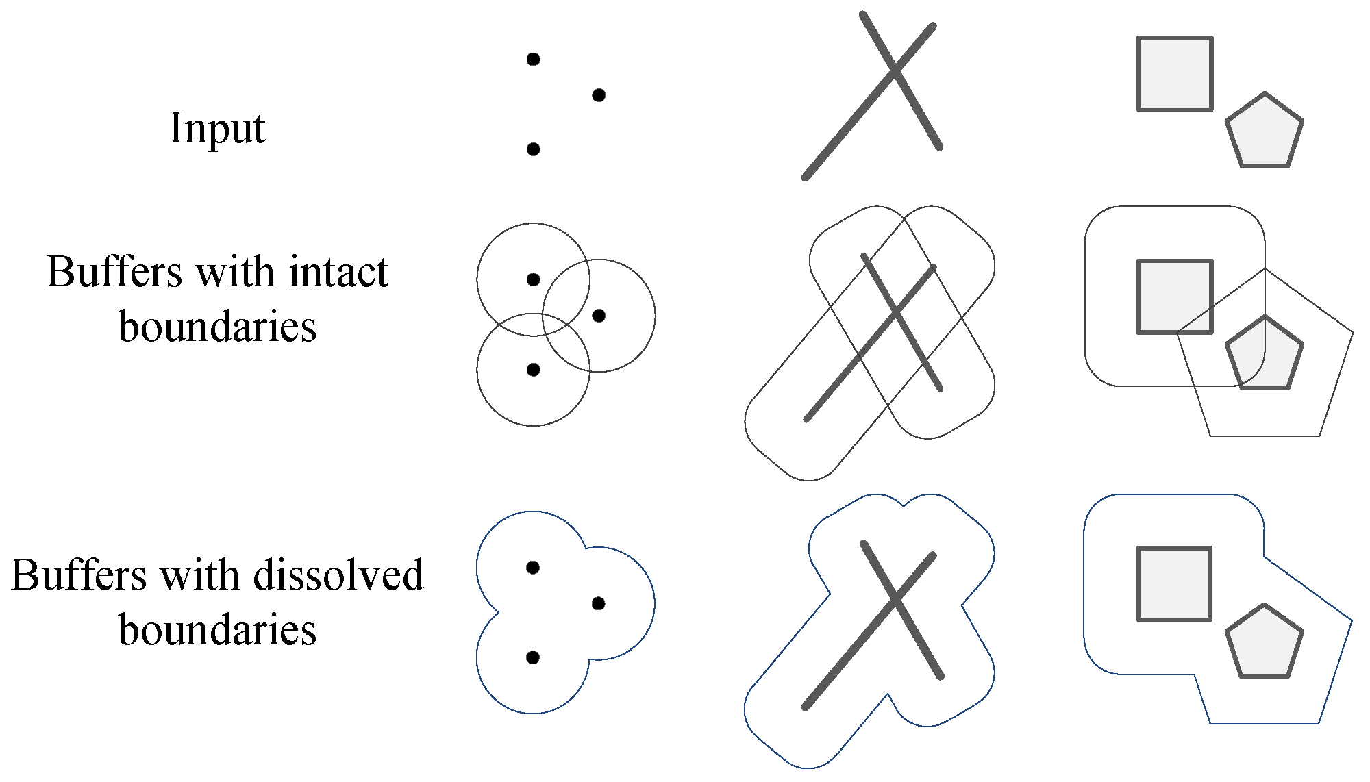
The vector buffer generation problem is solved in two steps: First, buffer zones are built for each object $d_i$ with a given buffer radius r. The single object buffer generation function is denoted as $F_{buffer}(d_i,r)$, and the entire result set of step one is expressed as $B=F_{buffer}(D,r)$, where B is the collection of all single buffer zones. Second, the buffer zones of the first step are dissolved into one (or several) integral polygons. The dissolve function is denoted as $F_{dissolve}\left(B\right)$. In this way, the buffer generation problem can be expressed conceptually as

$$F=F_{dissolve}\left(F_{buffer}(D,r)\right)$$

(1)

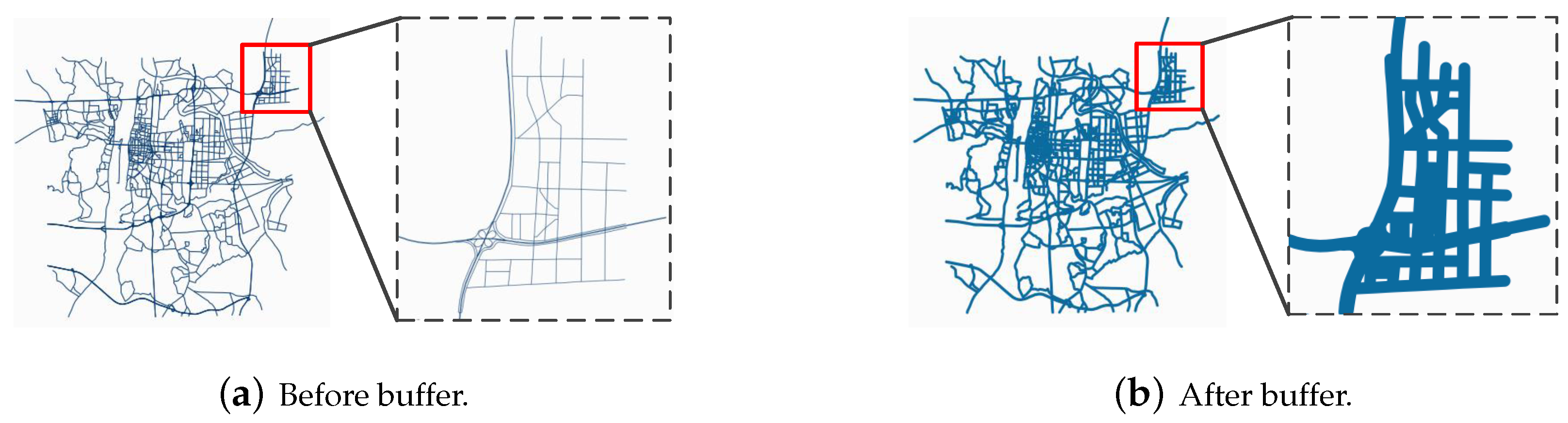
An example is shown in Figure 2, with a polyline dataset representing the road network of Changsha city in South China given in Figure 2a and the dissolved buffer result shown in Figure 2b. It could be observed that after the dissolving process, the result of the entire road network is a large and complex object.

Figure 2. Changsha city road buffer examples.

The dissolve procedure seems to be quite time-consuming. Therefore, a better solution may be achieved via parallelization. The most direct solution is to take the divide-and-conquer strategy: divide the input dataset D into multiple parts and calculate the dissolved results for each part until the final result is determined. We call each partition a data block, and the total number of blocks is denoted as p. Then, Equation (1) can be rewritten as Equation (2).

$$F=F_{dissolve}(\sum _{i=1}^p{F}_{dissolve}\left(F_{buffer}(D_i,r)\right))$$

(2)

Thus, the problem is turned into three steps. First, input dataset D is divided into p data blocks, each denoted as $D_i$. Second, the dissolved buffer zone of each data block is determined according to Equation (1); this step can be processed in parallel over p tasks. Third, the results from all data blocks are further merged into the final single geometry.

Regarding the above, there are some detailed problems. For example, in step one, the method for distributing D into p parts is unknown. Moreover, in later steps, an approach to merging each part into a larger one is lacking. To optimize the performance, the following three problems will be solved:

• Spatial Aggregation for Adjacent Data. After the mapping, $D\to \left\{D_i|i=1,2,\dots ,p\right\}$, the input dataset is divided into multiple data blocks. Clearly, the less overlap there is among these data blocks, the better the computing efficiency achieved later during geometry merging. By contrast, without spatial order, if the geographic range of a dataset is as broad as Russia or Canada, the buffer merge operations can be extremely costly. Therefore, the data objects should be partitioned according to their geographical proximity, namely, adjacent objects should be assigned to the same or a neighboring block.
• Data Blocks of Equal Size. The distribution of vector data in the real world is geographically unbalanced in two ways: the number of geographic objects in different areas is unbalanced and the number of vertices (a single geometry-like polyline or polygon contains a series of vertices) in different vector objects is unbalanced. The imbalance in data size causes an imbalance in the computing times of different parallel tasks. A method ensuring that each $D_i$ has roughly the same amount of data would cause the computational performance to be optimized on the whole. Thus, the optimization method should include the following considerations: (1) data splitting processing (to avoid a single large piece of data); (2) load balancing considerations regarding the total number of objects and the total number of vertices.
• Parallel Dissolving of Buffer Zones. The dissolving procedure $F_{dissolve}$ needs to be parallelized. While in MPI-based methods, the different processes are merged in a binary-tree-like way, in the Spark architecture, the data blocks are merged in parallel. Therefore, the best depth of the tree may be not ${\mathit{log}}_2\left(p\right)$. Moreover, the sequential order of p also needs to be maintained.

4. Methodology

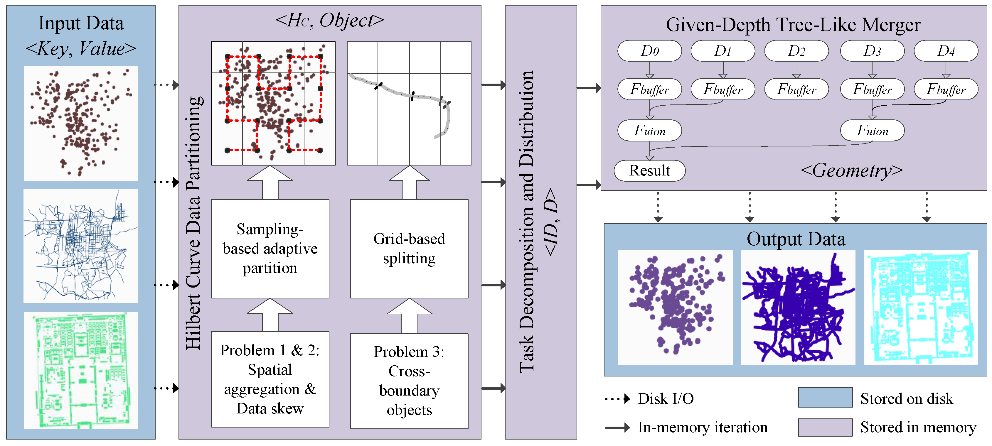
To overcome the drawbacks presented above, we propose a method based on the Hilbert filling curve to aggregate adjacent objects and thus to optimize the data distribution among all distributed data blocks and to reduce the cost of swapping data among different blocks during parallel processing. The method is called the HPBM (Hilbert curve partition buffer method), the framework of which is shown in Figure 3. There are three major phases of the HPBM: Hilbert-curve-based data partition, task decomposition and distribution, and depth-given tree-like merger.

Figure 3. Framework of HPBM.

Phase 1. Hilbert-curve-based data partition. In Spark, spatial data are stored in a distributed file system in $⟨Key,Value⟩$ form, where $Key$ represents the unique identifier of a single object and $Value$ includes a variety of attributes. First, the entire dataset is traversed by a Hilbert curve, and each object is encoded with a Hilbert code. Then, a sampling-based adaptive partitioning method is conducted to balance the data skew, and the boundary-crossing objects are addressed using a grid-based splitting strategy. After that, data objects are recoded in the new pair form $⟨H_c,d⟩$, with $H_c$ standing for the Hilbert code and d standing for other attributes of the object.

Phase 2. Task decomposition and distribution. Load balance is fully taken into consideration, and every partition is indexed with a unique identity. The data output in this phase can be presented as $⟨ID,D⟩$, which uses $ID$ as the sequential sorted number for data blocks.

Phase 3. Depth-given tree-like merging. First, every D is calculated to produce its result G using the equation $G_i=F_{buffer}(D_i,r)$. Then, after applying the dissolving operation $F_{dissolve}\left({\sum }_{i=1}^p{G}_i\right)$ to every data block, the final result is produced in a tree-like way.

4.1. Hilbert-Curve-Based Data Partition

In the parallel computing model, the data are distributed to different computing nodes to support simultaneous computations. Since buffer computation requires adjacent objects, it is necessary to avoid distributing spatially adjacent data to different computing nodes. The existing data allocation strategy is based on the ordinary grid partition strategy and does not satisfactorily aggregate adjacent spatial objects. In mathematical analysis, a space-filling curve (abbreviated as SFC in the following) is a curve whose range contains the entire n-dimensional unit hypercube. We found that space-filling curves have good advantages in terms of the aggregation of neighboring spatial objects when compared with an ordinary grid [14]. Space-filling curves in parallel buffer analysis has not been addressed in recent research [16,17,32], though in his literature [17], Fan presented this topic as a future research direction. Therefore, we present a more efficient partitioning method based on space-filling curves, which essentially contains two steps.

Step 1: Hilbert-curve-based spatial aggregation. Types of space-filling curves include the Peano curve, the Hilbert curve, and the Z-order curve. Among all space-filling curves, the Hilbert curve is superior in terms of spatial aggregation [36].

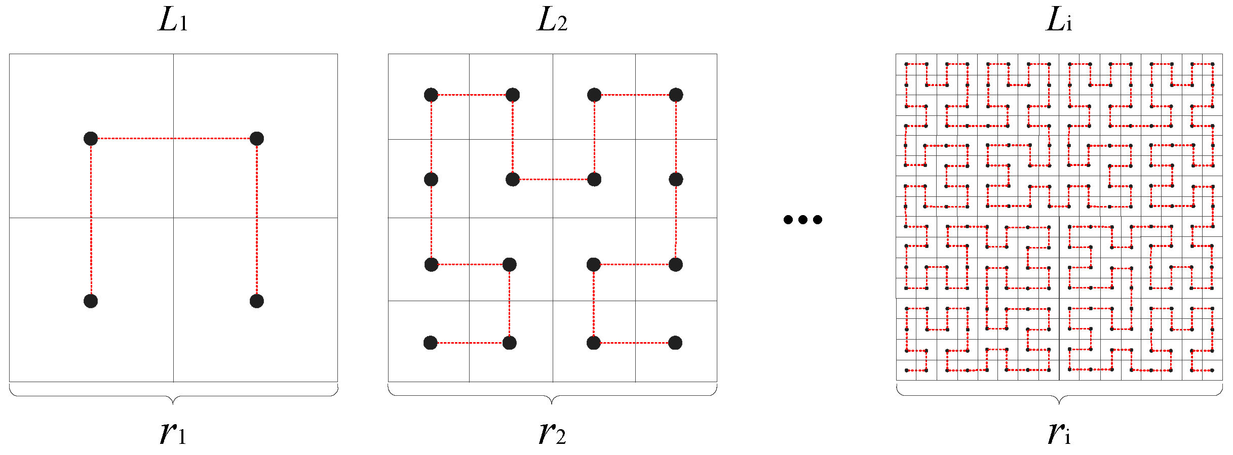
First, the plane space is described using k layers of different resolutions. Each layer is denoted as $L_i(i\in [1,k])$ and is divided into $R_i\times R_i$ grids to support parallel task allocation, where $R_i$ is called the resolution and $R_i=2^{L_i}(i\in [1,k])$; the grids are denoted as $U=\left\{U_i|i=1,2,\dots ,R_i^2\right\}$. Each layer $L_i$ is filled with an ith-order Hilbert curve, as shown in Figure 4.

Figure 4. Hierarchical space partition schema.

Then, the Hilbert code of each grid in $L_i$ can be calculated based on the Hilbert curve coding method proposed by Faloutsos [37].

The vertices of the $LINE$ and $POLYGON$ objects in $U_i$ are given the same Hilbert code, i.e., $U_i$. Thus, we build a mapping function (Equation (3)) to map each vertex of the spatial objects to its corresponding Hilbert code, where $H_c$ denotes the Hilbert code, $f_h$ is the mapping function, $L_i$ is the corresponding layer, and X and Y denote the longitude and the latitude of the vertex, respectively.

$$H_c=f_h(L_i,X,Y)$$

(3)

While the $⟨Key,Value⟩$ model fits nicely with large-scale data via SFC $Key$-based partitioning, spatial analytics are intrinsically complex due to their multidimensional nature [18]. There are two remaining major problems to address: the spatial data skew problem and boundary object problem. The latter problem is solved in the next subsection.

Algorithm 1 Adaptive Hilbert-Based Data Partition Algorithm.
Input: D: input data; $L_j$: initial layer; $C_{max}$: maximum number of objects allowed in a grid;
Output: matched Hilbert layer number j;
1:	if $\mathit{D.type}=\mathit{POINT}$ then
2:	sample D with ratio $Sa$;
3:	end if
4:	if $\mathit{D.type}=\mathit{LINE}$ then
5:	split single line into a series of v;// v denotes vertex, which is regarded as a single point
6:	sample the series of v with ratio $Sa$;
7:	end if
8:	for $j<k$ do //k is the maximum layer allowed
9:	initialize the $SFC$ according to $L_j$;
10:	compute $H_c$ for every sampled point according to Equation (3);
11:	count the number of objects in every grid and choose the largest one as $U_{max}$;
12:	if $U_{max}/Sa>C_{max}$ then //$U_{max}/Sa$ is the estimated value
13:	$j=j+1$;
14:	else
15:	return j;
16:	end if
17:	end for

Step 2: Spatial data skew processing. From the OpenStreetMap dataset, we take the Beijing POI (point of interest) data for experiments. By partitioning the space at level $L_i$ into grids U with resolution $R_i=12$, the average number of objects per grid is 522, with the largest number in a grid being 35,036. If buffer generation calculation is based on the combined data block of the grids, the response time can increase significantly due to these “huge” grids.

As analyzed above, there should be a threshold regarding the maximum number of objects $C_{max}$ allowed for a single grid. To achieve this goal, an adaptive data-partitioning-level-setting algorithm is proposed [18]. However, the count operation in the algorithm incurs an increase in both computation and I/O. In our other studies, we found that the sampling methods could reduce resource consumption. Therefore, we propose estimating and approximating the entire dataset via sampling. In our method, $U_{max}/Sa$ is used to estimate the original data, where $Sa$ denotes the sampling ratio. $U_{max}/Sa$ provides an unbiased estimation since the random sampling strategy is applied.

The final algorithm is described in Algorithm 1. On the basis of the selected SFC, the qualified layer number j is finally output after completing the recursive calculations.

4.2. Boundary Object Processing

In the partition operation, grid-crossing objects may occur. To improve the processing speed, an appropriate strategy is needed to address this event.

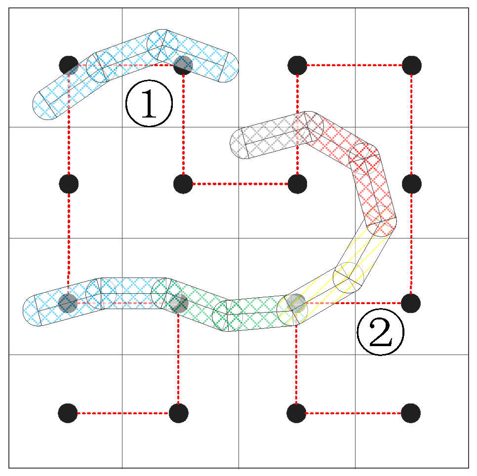
Spatial objects that cross over the grid boundaries are called boundary objects. For $POINT$ objects, this does not occur. However, some $LINE$ objects can cross multiple grids. As shown in Figure 5, line 1 crosses over two grids, while line 2 crosses over six grids. This phenomenon raises the following two problems. First, to which grid does the object belong? Second, load unbalance occurs as a result of these objects because the clipping operation is sensitive to the number of vertices.

Figure 5. Boundary object processing example.

Multiple matching methods and multiple assignment methods are adopted to address these issues [18,38]. They work perfectly for the spatial query and join operations, despite the slightly increased overhead in the latter method due to the multiple duplications. Though they remain effective when used for $POINT$ buffering, they become less capable in $LINE$ buffer analysis. For example, the multiple match does not eliminate the load unbalance problem because single large data remain unchanged. Worse still, the multiple assignment method, which duplicates boundary objects for multiple grids, causes storage overhead and extra I/O.

Since $LINE$ buffer analysis is much more sophisticated, neither multiple matching nor multiple assignment helps to solve this problem. For this reason, we propose splitting the single line vector objects into line segments. This strategy is practically supported in two ways. Primarily, the splitting-and-conquer method is one of the ways to create a buffer zone [17]. Moreover, the topology relationship between split lines is insignificant for the dissolve-type buffer result.

Therefore, a new approximation grid segmentation method is put forward, the procedure of which is introduced in Algorithm 2. A threshold F for detecting the number of vertices in one object is set. The total number of vertices in the object over F is split, while the remaining ones are retained. For those objects that are not split up, the Hilbert code of the middle vertex $H_c\left(v_i\right)=f_h(L_i,v_i.X,v_j.Y)$ is chosen as the $Key$. For those that are split up, the entire line object is decomposed into an array of small segments that run through at least two grids. Figure 5 gives an example; if F is set to 5, then line 1 is unchanged, while line 2, where the vertices are numbered from left to right, is cut into five short lines.

Algorithm 2 Boundary Object Assigning and Splitting Algorithm.
Input: D: input line dataset; $L_i$: the level of the layer of the given $SFC$; F: vertices number threshold;
Output: $D^{\prime }$: new line dataset;
1:	$D^{\prime }=\varnothing$
2:	for each d in D do
3:	compute the number of vertices in d: $len\left(d\right)$;
4:	if ($len\left(d\right)$ <= F) then
5:	$H_c\left(d\right)=f_h(L_i,v_j.X,v_j.Y|j=\lfloor len\left(d\right)/2\rfloor )$; //compute Hilbert code with middle vertex of d
6:	Append $⟨H_c,d⟩$ into $D^{\prime }$;
7:	else
8:	$j=1$;
9:	$v_s=v_j$;
10:	while ($v_j\ne v_{len\left(d\right)}$) do
11:	if ($H_c\left(v_j\right)\ne H_c\left(v_{j+1}\right)$) then
12:	split the line and create a new line $d^{\prime }$, with vertices from $v_s$ to $v_{j+1}$;
13:	$H_c\left(d^{\prime }\right)=H_c\left(v_j\right)$;
14:	Append $⟨H_c,d^{\prime }⟩$ into $D^{\prime }$;
15:	$v_s=v_{j+1}$;
16:	end if
17:	$j=j+1$;
18:	end while
19:	end if
20:	end for
21:	return $D^{\prime }$

4.3. Grid-Based Accumulative Data Decomposition

When many small grids are merged into a series of large data blocks D, decomposition is achieved for the previously partitioned data. Afterwards, the batch products can be processed in parallel. However, two problems need to be taken into consideration in this step. First, too many small series D lead to deteriorated performance [18]. This problem may occur during grid partition and decomposition [14], as there is no recursive partition strategy. Thus, the grids may be densely partitioned and decomposed. Second, a single high-density partitioned series D may require a lengthy calculation time, thereby causing processing congestion. To solve this problem, an even decomposition strategy, which decomposes the data according to the number of vertices, is utilized [16,17,32].

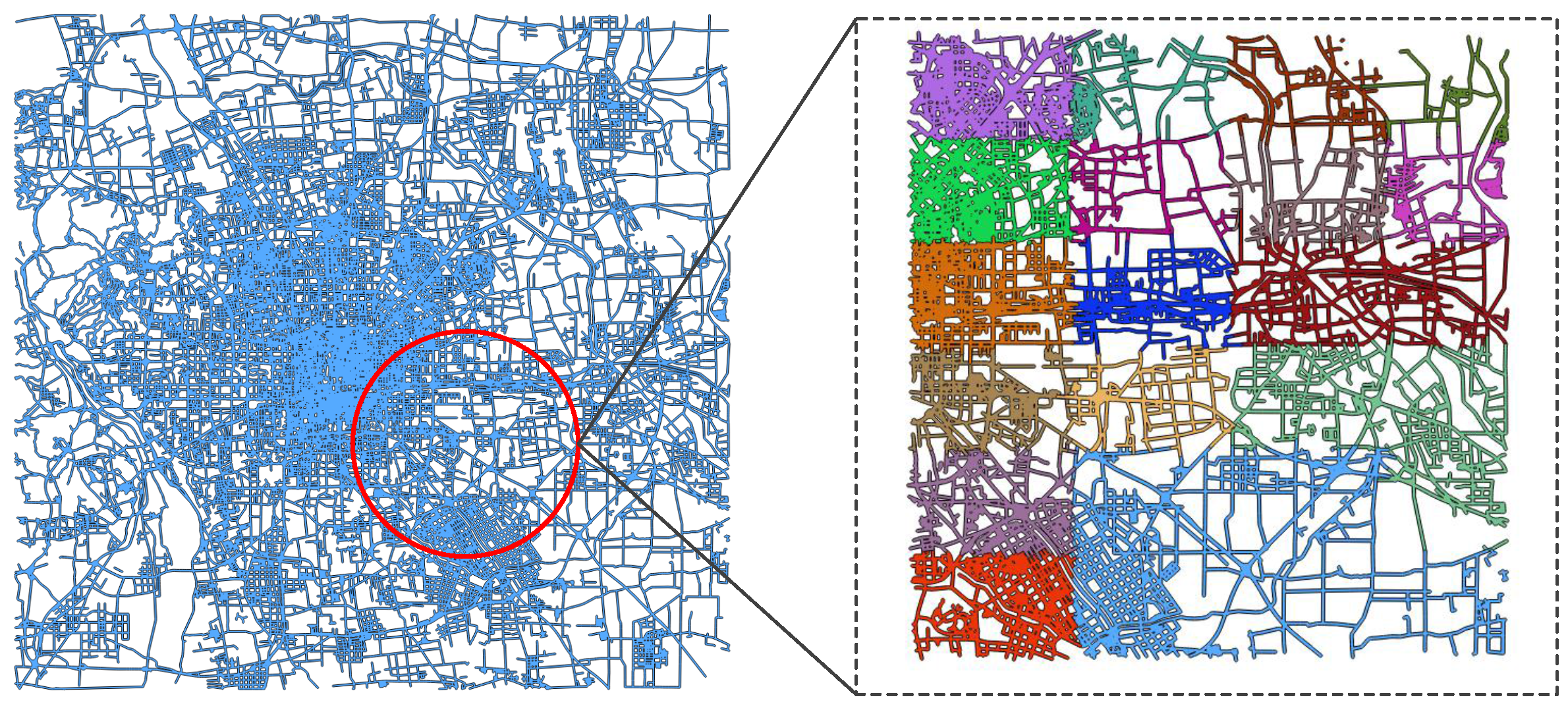
Our goal is to minimize the chances of producing a single large data block as well as control the total number of data blocks. The task decomposition algorithm consists of three steps. First, the spatial aggregation attribute is acquired by sorting $⟨H_c,d⟩$, and the number of objects in every grid is counted. Second, according to the total count, we evenly put them into p parts. We note that the value of p should be neither too small nor too large, as explained above. Third, each data block is indexed with a unique $ID$, as the order of the $ID$s also indicates the spatial aggregation attribute for D. The example is illustrated in Figure 6; the Beijing road data are divided, with colors used to distinguish the decomposed data blocks. As we can see, sparsely distributed data contain more grids and vice versa.

Figure 6. Buffer result and partial data splitting example.

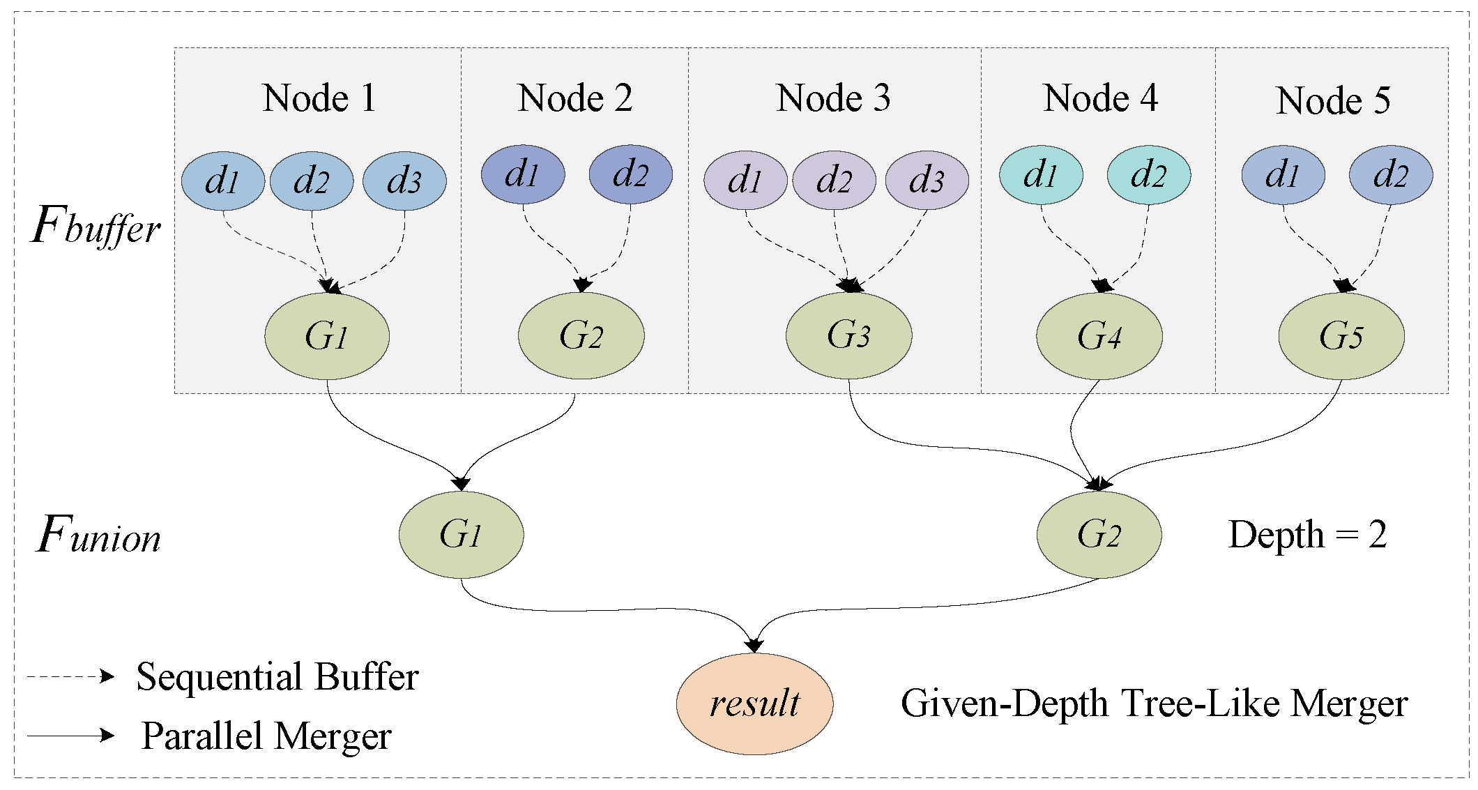
4.4. Buffer Generation and Depth-Given Tree-Like Merging

In step ${\sum }_{i=1}^p{G}_i$, with $G_i=F_{dissolve}\left(F_{buffer}(D_i,r)\right)$, the dissolved buffer zone of various datasets D is calculated to produce G. This step can provide significant advantages over parallel computing, as the I/O from different nodes are rarely involved. However, the later step, $F_{dissolve}\left({\sum }_{i=1}^p{G}_i\right)$, requires combining all of the G, for which a suitable parallel merger strategy is required.

The previous parallel merger methods—the binary-tree-like merger method, compared with the sequential merger method—are more superior at large. This is mainly because they make the most use of multi-cores and reduce the congestion [16,17]. However, the previous two tree-like methods are based on MPI processes, thus making scalable computing difficult to achieve due to the complexity of multiprocess programming.

The merger method in Spark can be rather different from that of the MPI for the following reasons. First, in the MPI-based method, the datasets D are divided into c parts, where c denotes the number of processes. However, they are divided into p parts in our method, with $p>c$, where p is not affected by the number of processes. Second, the depth $h=lo{g}_2\left(c\right)$ of the MPI-based methods is not suitable for our method herein. Third, every file block also has a geolocation attribute, which calls for the full use of the $ID$. Therefore, we apply the data-block-based tree-like method and not the processed-based tree-like method.

On this basis, this paper uses the depth-given tree-like buffer merger method. The purpose of this method is to reduce the number of intermediate results, as well as make the most of the geoinformation of data blocks. In this way, the high cost of geometric consumption is alleviated. As shown in Figure 7, the whole procedure is mainly divided into two steps. After subsets D are partitioned into nodes 1–5, the dissolved buffer zone G is generated within every node. Then, several G are merged in a tree-like way, with the given depth equal to 2.

Figure 7. Depth-given tree-like merger example.

There are two important parameters in this step: the depth parameter h and the fanout parameter b. Their relationship is represented by Equation (4). b is used to calculate the remaining data blocks after every layer of merger. For example, after the first merger, the remaining number of G is $\lfloor p/b\rfloor$, and after the second merger, the remaining number of G is $\lfloor \lfloor p/b\rfloor /b\rfloor$.

$$b=max(\lceil p^{\frac{1}{h}}\rceil ,2)$$

(4)

In our algorithm, b is fixed at 3. This setting means that $\lceil p^{\frac{1}{h}}\rceil =3$, which further implies that h is slightly smaller than $lo{g}_2\left(p\right)$. This setting guarantees the comparatively best performance. To demonstrate the function of this setting, the cost function is used to give a direct explanation. The cost function consists of three parts: computation cost, dissolving cost, and I/O cost. The parameter b is set to 2, 3, and 4 (or $>4$).

If b is set to 2, a waiting period does not exist in the dissolving process, which makes the computation cost low. However, the number of intermediate results is much larger than that for a higher value of b, which results in a high dissolving cost. Thus, its I/O is also the highest among the three methods.

If b is set to 3, a waiting period does exist in the dissolving process, as 3 blocks are sequentially dissolved, which leads to a higher computational cost. Meanwhile, the dissolving cost and I/O cost decrease because the number of intermediate results is reduced.

If b is set to 4, a longer waiting period exists in the dissolving process, as 4 blocks are sequentially dissolved; thus, the efficiency is decreased significantly.

Subsequently, our objective is to finish the computation as fast as possible. If $b\ge 4$, then the larger the value of b, the larger the waiting time cost of the dissolving process. If $b=2$, the comparatively high dissolving cost and I/O cost lead to a deteriorated performance. Therefore, $b=3$ is the theoretically better choice for parallel buffer generation.

5. Performance Analysis

In this section, we analyze the computational complexity of the whole algorithm. The whole algorithm is divided into four steps: data partition, data decomposition, local buffer and dissolve, and global dissolve. It is acknowledged that the local buffer and global buffer are the most time-consuming steps, as these operations are the most computationally intensive.

For the input data, the number of objects is N; the total number of vertices is V; the number of data blocks is p; the sampling operation is expressed as $S_a(·)$; the Hilbert code calculation is expressed as $H_c(·)$; the buffer operation is denoted as $F_{buffer}(·)$; and the dissolve operation is denoted as $F_{dissolve}(·)$. The whole cost of our method is $O(S_a\left(N\right)+H_c\left(N\right)+R\left(N\right))+O\left(N\right)+F_{dissolve}\left(F_{buffer}(N+N_e(e-1))\right)+F_{dissolve}\left(lo{g}_b\left(p\right)\right)$.

Data Partition. Data partition means to partition the data according to our adaptive Hilbert-based data partition algorithm. In this algorithm, we assume that the data are partitioned once and that the cost is $O(S_a\left(N\right)+H_c\left(N\right)+R\left(N\right))$. $O\left(S_a\left(N\right)\right)$ represents the cost of finding suitable partition layers for the sampled data, $O\left(H_c\left(N\right)\right)$ represents the Hilbert code calculation and $O\left(R\right(N\left)\right)$ represents sorting according to $H_c$.

Data Decomposition. Data decomposition means to decompose all the data into a series of data blocks and to distribute them to different computing nodes. This step requires one iteration of all the data, the cost of which is $O\left(N\right)$, which is the most insignificant among the four steps.

Local Buffer and Dissolve. For this step, it is difficult to give the precise cost expression due to the uniqueness of different spatial data. Thus, the complexity is expressed approximately. e represents the average number of grids crossed for every single object, and $N_e$ represents the crossing-boundary objects. Apparently, the number of objects is $N_e(e-1)$, and the number of vertices is $N_e(e-1)$. Therefore, the cost of our method is $O\left(F_{dissolve}\left(F_{buffer}(N+N_e(e-1))\right)\right)$.

Global Dissolve. Apparently, in the MPI-based method, using the binary-tree-like method, the cost decreases from $O\left(c\right)$ to $O\left(lo{g}_2\left(e\right)\right)$, and all union times can be represented as $2^{lo{g}_{2}e}-1$. Regarding our method, the computational cost is reduced from $O\left(p\right)$ to $O\left(lo{g}_b\left(p\right)\right)$, the base b is calculated using Equation (4), and the new union times can be represented as $\frac{b(1-b^h)}{1-b}$. The cost of our method is $O\left(F_{dissolve}\left(lo{g}_b\left(p\right)\right)\right)$. Thus, the resource consumption is optimized and reduced.

6. Experimental Evaluation

We conducted several experiments to measure the impacts of different strategies, including the partition method, cross-grid object handling method, and depth-given tree-like merger method. Finally, we compared the HPBM with three other algorithms [16,17,32]. Different from the method applied in Reference [17], we did not construct an R-tree, as there was no need to filter the data.

6.1. Experimental Setup and Datasets

Experiments were conducted in two different environments—stand-alone and cluster. The code was implemented using the Scala language. The experiments were based on Spark 1.6.1, Hadoop 2.6, and JDK 1.8. Some other open-source GIS software programs were utilized: QGIS version 2.0, PostGIS version 2.1, Citus Data version 5.2, and ArcGIS 10.2. The experimental hardware environment is shown in Table 2.

Table 2. Hardware environment.

Item	Stand-alone	Cluster
CPU	32 core, Intel(R) Xeon(R) E5-4620 @ 2.60 GHz	5 × 20 core, Intel(R) Xeon(R) E5-2650 @ 2.30 GHz
Memory	256 GB	5 × 256 GB
OS	Centos 7.1	Centos 7.1

Table 3 shows the OpenStreetMap datasets used in these experiments. All files were saved in “CSV” format. More importantly, all the data were collected from the real world and have the geographically unbalanced distribution property. Apparently, such data create challenges with respect to efficient processing.

Table 3. Datasets used in the experiment. OSM: OpenStreetMap.

Dataset	Abbreviation	Records	Vertices
$\mathrm{OSM}\mathrm{Beijing}\mathrm{business}\mathrm{point}$	$P_1$	66,511	66,511
$\mathrm{OSM}\mathrm{Beijing}\mathrm{point}$	$P_2$	251,282	251,282
$\mathrm{OSM}\mathrm{Beijing}\mathrm{road}$	$L_1$	40,927	244,340
$\mathrm{OSM}\mathrm{Taiwan}\mathrm{road}1$	$L_2$	84,413	969,298
$\mathrm{OSM}\mathrm{Taiwan}\mathrm{road}2$	$L_3$	208,067	2,244,317
$\mathrm{OSM}\mathrm{Switzerland}\mathrm{road}$	$L_4$	597,829	6,359,119

Experiments 1–3 were carried out in the stand-alone environment. Experiment 4 involved the algorithm comparisons that were carried out in both the stand-alone and cluster environments to verify the scalability of the HPBM. In all the experiments, the buffer distance r was set to 200 m, which has practical meaning for those datasets with a wide spatial range.

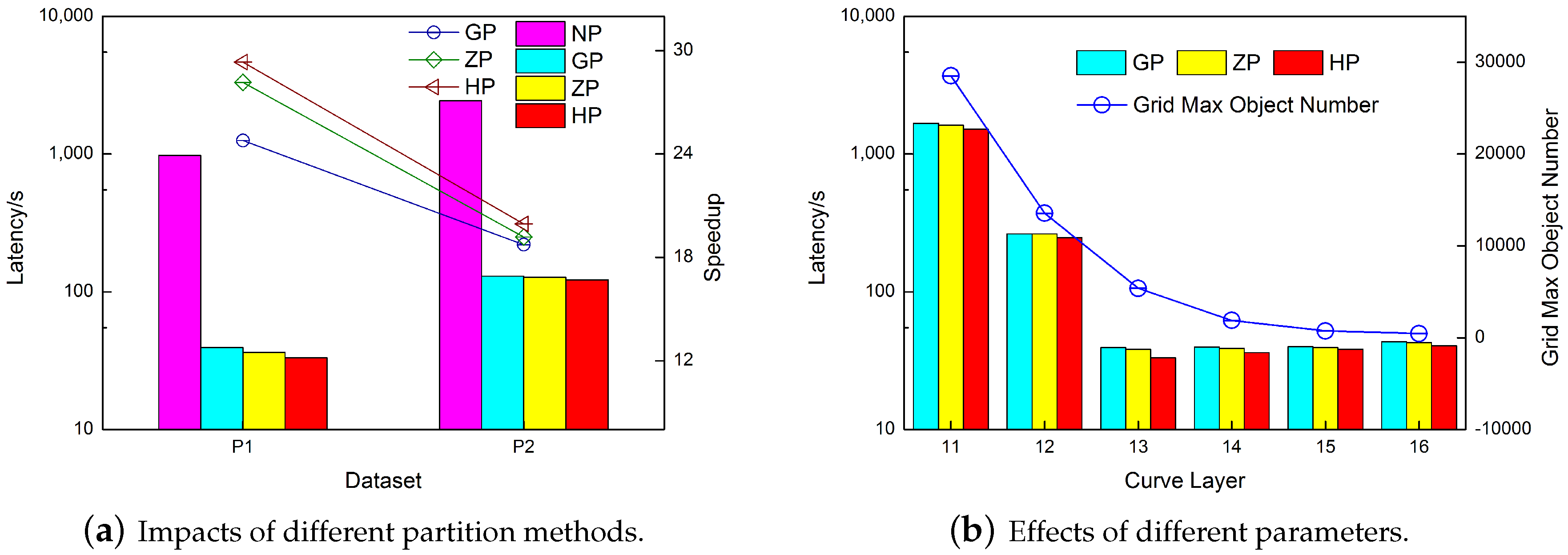
6.2. Experiment 1. Impact of Partition and Cross-Boundary Object Handling Method

Experiments settings. To evaluate the performance gain of the Hilbert curve used in the HPBM, experiments were conducted on the four methods shown in Table 4. They were all adopted for experiments on the $P_1$ and $P_2$ datasets, and the resolutions of the grids were set to be identical.

Table 4. Method comparison in experiment 1.

Abbreviation	Method
NP	no partition
GP	grid partition
ZP	Z-curve partition
HP	Hilbert curve partition

As shown in Figure 8a, the result demonstrates the necessity of implying a geographical partition strategy and the correctness of using the Hilbert-curve-based partition method. The three partition methods are more than one order of magnitude faster than NP, regardless whether considering $P_1$ or $P_2$. In terms of GP, ZP, and HP, the efficiency of the HP method is slightly higher, as implied by the speedup lines (comparison with NP). The superior spatial adjacent attribution of the Hilbert curve was demonstrated [36]. In our experiment, the efficiency of the Hilbert partition for parallel buffer analysis was tested.

Figure 8. Experiment on cross-grid data processing methods.

To verify the necessity of the adaptive spatial filling curve hierarchy, we continued to experiment on the $P_2$ dataset with different $SFC$ layers. The results are shown in Figure 8b. All three methods were affected by the curve level with roughly the same trend. When the level was too low, the amount of data in a single grid could be quite large, having apparent different effects. In contrast, when the level became too high, the excessively dense partition increased the amount of calculation, though less significantly.

6.3. Experiment 2. Cross-Grid Data Processing Method

Experiments settings. In this experiment, we compared the 4 methods shown in Table 5. In the DS method, the objects are divided into many single segments, which are regarded as single new lines. $POINT$ data are seldom affected by the boundary-crossing problem; thus, only $LINE$ datasets were used to carry out this experiment. In addition, the replication method is more complex than the arbitrary assignment method; thus, it was not tested.

Table 5. Method comparison in experiment 2.

Abbreviation	Method
NP	no partition
AA	arbitrary assignment method
DS	divide-and-conquer split method
AS	approximate split method

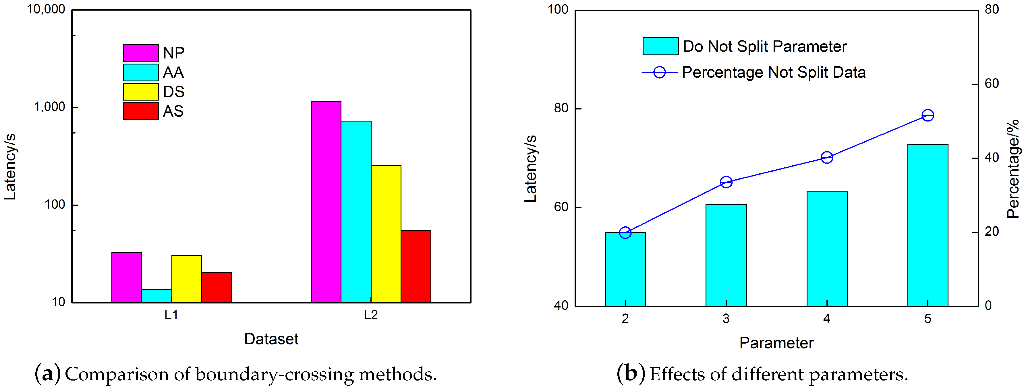
The experimental results are shown in Figure 9a. The performance gain of AS is obvious, especially when the amount of data is large enough. When addressing $L_1$, AA outperforms the other 3 methods; this trend is explained in Section 5. Regarding $L_2$, AA falls to third place, while AS becomes first. This dramatic change is caused by the dataset property. There exists a higher percentage of single long data in $L_2$ compared with $L_1$, for which the splitting methods would be more effective. Regarding the NP method, it demonstrates the necessity of optimization.

Figure 9. Experiment on cross-grid data processing methods.

For the AS method proposed in this paper, the influence of its own parameters was also verified. In this experiment, line lengths below the given threshold were not cut. The results are shown in Figure 9b. For data with a node number less than 3, the best computational efficiency could be obtained when the threshold $F=2$.

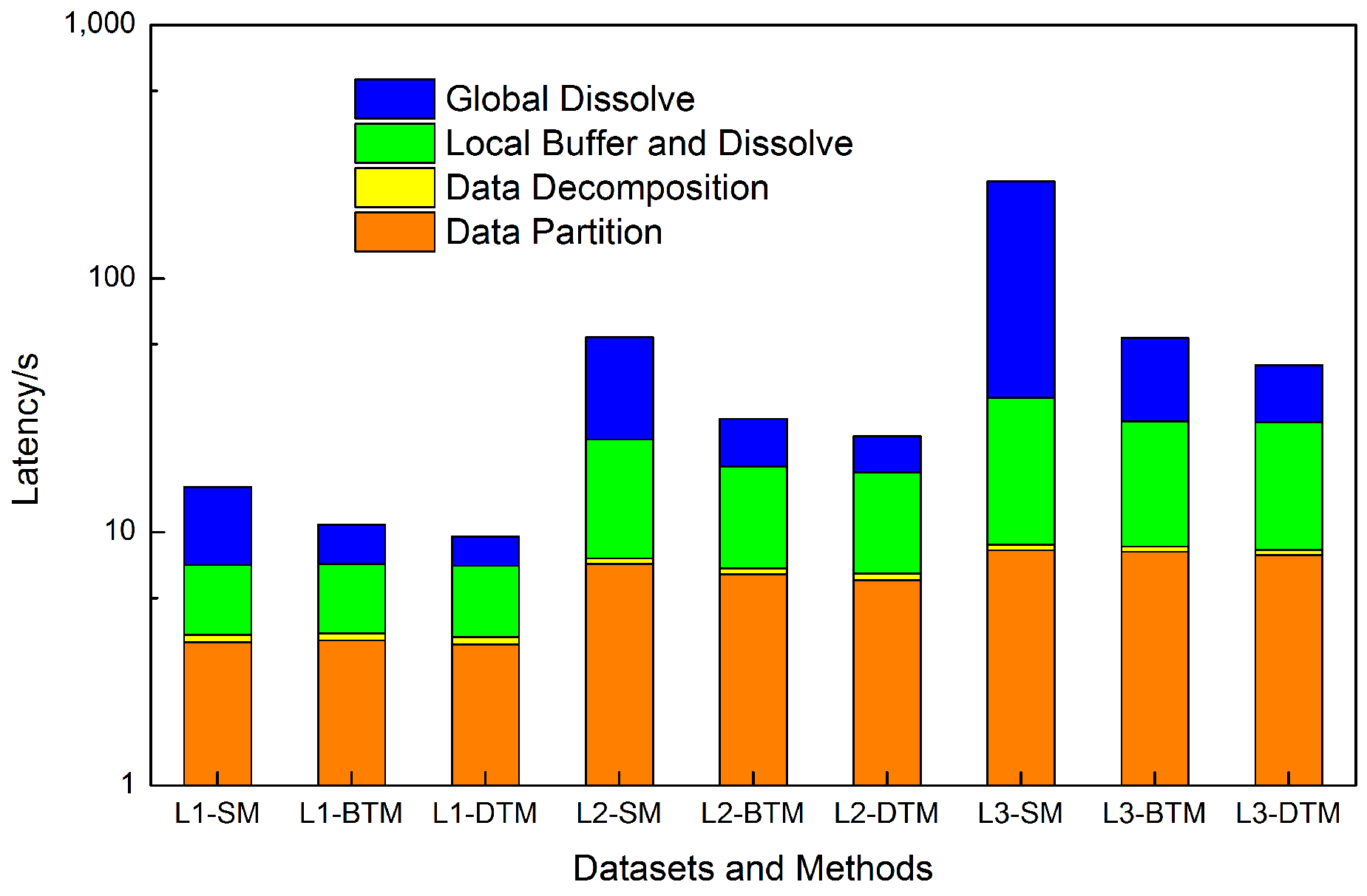
6.4. Experiment 3. Comparison of Tree-Like Merger Methods

Experiments settings. As shown in Table 6, 3 methods were tested on $L_1$, $L_2$ and $L_3$. The $DTM$ is the strategy used in our paper.

Table 6. Method comparison in experiment 3.

Abbreviation	Method
SM	sequential merger
BTM	binary-tree-like merger
DTM	depth-given tree-like merger

The results are shown in Figure 10, where the timings of four different components are listed. Seen from the whole procedure, the two tree-like merging methods are apparently superior to the sequential merging method. When focusing on different timings, we note that the time costs of the data partition, data decomposition, and local buffer and dissolve for these three methods are approximately the same. By contrast, a significant difference exists in terms of the global buffer; this difference becomes even more significant as the dataset becomes larger. For the SM method, the one-by-one merger strategy brings about an obviously long waiting time, especially for large dataset $L_3$. Regarding the two tree-like methods, the DTM is slightly better than the BTM when a smaller depth h is used for the BTM than that of the DTM. This result clearly demonstrates that the DTM can reduce the intermediate results and network overhead.

Figure 10. Experiments on the tree-like merger methods.

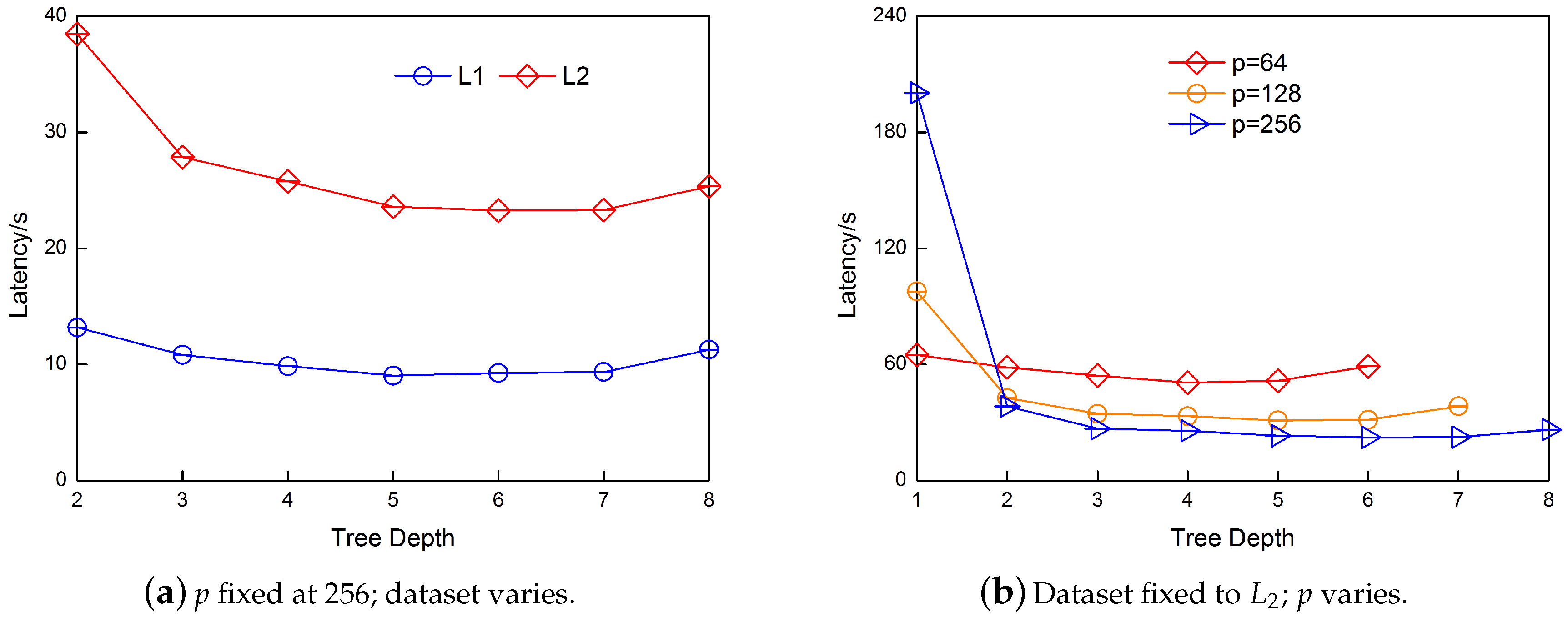
The relationship between h and the number p is also experimentally verified. Figure 11a illustrates the correctness of our depth setting. When p is fixed to 256, regardless of the size of the dataset, the optimal depths of h are 5, 6 and 7 ($b=3$). Such result is in accordance with our analysis in Section 4. Moreover, if h becomes smaller, more computation time is consumed.

Figure 11. Experiment on the parameters.

Similarly, when the dataset is fixed to $L_2$, the results are as shown in Figure 11b. These results also support the conclusion in Section 4. If p changes, h will also change. When $p=64$, the best h is 4 and 5. When $p=128$, the best h is 5 and 6. When $p=256$, the best h is 5, 6 and 7. Moreover, the performance improves as the number of data blocks p increases.

6.5. Experiment 4. Algorithm Comparison Experiment

Comparison algorithms. Algorithm comparison experiments were carried out in both the stand-alone and cluster environments. If the running time was more than 2 h or the algorithm failed to return a result, the result was not be recorded due to a lack of practical application value.

Algorithms 1 [17], 2 [16], and 3 [32] mainly adopt the strategies previously mentioned in the referred articles. We have to admit that they are not equivalent to the original methods for the following two reasons. First, our experimental environment is different from theirs. Second, one of the most important factors in buffer analysis, the buffer distance r, is not given in those references. Under these circumstances, we optimized Algorithms 1–3 to produce Optimized Algorithms 1–3 by adopting our Hilbert curve partition method. Our reasons for this optimization are listed below. First, the optimizing effect of the Hilbert curve partition is verified in Experiment 1. In addition, adding this strategy enables some algorithms to address large-scale data; for example, Algorithm 3 has not yet been tested on datasets larger than 10,000 objects, but it shows the capability to tackle $L_3$ as a result of our optimization. Finally, the effectiveness of other optimization methods can be seen and analyzed more clearly herein.

• OA1. OA1 (Optimized Algorithm 1) is based on three optimization methods: split-and-conquer buffer zone generation, vertices-based task decomposition, and tree-like merger [17].
• OA2. OA2 (Optimized Algorithm 2) adopts strategies such as vertices-based task decomposition and tree-like merger [16].
• OA3. OA3 (Optimized Algorithm 3) uses the equivalent-arc partition strategy [32].
• A4. A4 (Algorithm 4) is the general parallel buffer method, as depicted in Section 3 (method before optimization).

Stand-alone Settings. In the experiment, we compared the HPBM with OA 1–3, A4, and the popular GIS software programs PostGIS, QGIS and ArcGIS. The results are shown in Table 7.

Table 7. Stand-alone experiment. GIS: geographic information systems; HPBM: Hilbert curve partition buffer method.

Algorithm	${\mathbf{L}}_1$		${\mathbf{L}}_2$		${\mathbf{L}}_3$		${\mathbf{L}}_4$
	Latency/s	Speedup	Latency/s	Speedup	Latency/s	Speedup	Latency/s	Speedup
HPBM	9.041	/	22.366	/	38.787	/	332.346	/
OA1	15.443	1.7	70.831	3.2	128.195	3.3	936.889	2.8
OA2	12.299	1.4	41.086	1.8	75.515	1.9	661.857	2.0
OA3	17.183	1.9	81.491	3.6	220.771	5.7	2813.385	8.5
A4	234.190	25.9	587.594	26.3	6059.45	156.2	×	×
PostGIS	34.945	3.9	102.910	4.6	295.836	7.6	2380.201	7.2
QGIS	129	14.3	503	22.5	2788	71.9	×	×
ArcGIS	139	15.4	477	21.3	2365	61.0	×	×

For a small dataset such as $L_1$, the optimization benefits for the HPBM and OA1–3 are conceivable. The result of OA1 is slightly inferior to that of OA2, as its buffer zone generation strategy causes a large number of extra union operation costs. Regarding OA3, its bottlenecks arise from the one-by-one merger strategy. Not surprisingly, the non-optimized method A4 is the slowest. Albeit less significantly, the efficiency of the database GIS method PostGIS exceeds that of QGIS and ArcGIS.

Compared with $L_1$, $L_2$ contains a higher percentage of single long data. Such spatially unbalanced data make splitting single long data necessary. The HPBM adapting splitting methods bestow apparent benefits in terms of the global buffer, as analyzed in experiment 3. Compared with OA2, OA1 suffers from its own split-and-conquer drawbacks. Finally, among the three GIS software programs, PostGIS enjoys a better performance.

Not surprisingly, the analysis of $L_3$ is roughly the same as that of $L_2$. However, we have to note that OA3 is capable of handling larger amounts of data after our Hilbert partition method is applied. However, OA3 experiences more severe congestion when more data blocks are created for this larger amount of data. Compared with the other methods, A4 requires a drastically long computation time, mainly because the spatial aggregation attribute is not taken into consideration.

In larger dataset $L_4$, there are 597,829 objects. Although the computational complexity increases greatly, the HPBM outperforms the other methods by more than 50% and achieves speedups of 2.8, 2.0, 8.5, and 7.2 times that of OA1, OA2, OA3, and PostGIS, respectively. By contrast, A4, QGIS and ArcGIS are not capable of finishing the calculation or cannot do so within 2 h. Moreover, in OA3, the equivalent-arc data block partition method exhibits a limited optimization effect when addressing large amounts of data. To our surprise, PostGIS behaves even better than OA3.

Overall, the improved strategies offer more pruning and optimization opportunities.

Cluster Settings. To demonstrate the scalability of our method, the same experiments were carried out for a cluster with 100 cores. Citus Data extends PostGIS such that it supports the distributed computing. The buffer generation method in Citus Data consists of two steps. Step 1: all data are partitioned and distributed to all the slave nodes; then, the dissolved buffer zone is generated for every slave node. Step 2: all the dissolved buffer results of the slave nodes are transmitted to the master node for reunion to produce the final result. The results are shown in Table 8.

Table 8. Cluster experiment.

Algorithm	${\mathbf{L}}_1$		${\mathbf{L}}_2$		${\mathbf{L}}_3$		${\mathbf{L}}_4$
	Latency/s	Speedup	Latency/s	Speedup	Latency/s	Speedup	Latency/s	Speedup
HPBM	10.334	/	18.523	/	26.859	/	172.889	/
OA1	17.041	1.6	42.874	2.3	84.311	3.1	672.722	3.9
OA2	14.266	1.4	26.44	1.4	75.515	1.9	661.857	2.0
OA3	19.082	1.8	71.226	3.8	280.771	10.5	2534.29	14.7
A4	200.189	19.4	478.331	25.8	4410.555	164.2	×	×
$\mathrm{Citus}\mathrm{Data}$	20.134	1.9	61.51	3.3	200.436	7.5	×	×

Regarding the small dataset $L_1$, two features of the distributed parallel computing environment should be taken into consideration. The I/O expenses between different nodes cause a decrease in the computation efficiency. In addition, using too many cores results in significant task-startup overhead. Therefore, as seen from the figure, the comprehensive performances of the HPBM and OA1–3 are even a little inferior to those in the stand-alone environment, with an average drop of 13%. In contrast, Citus Data enjoys significant speedup because of the distributed $F_{buffer}$.

For the larger dataset $L_2$, the execution efficiencies of the HPBM and OA1–3 improve significantly, outperforming those in the stand-alone environment.

Regarding $L_3$, when compared with the experiment in the stand-alone environment, the performances of the HPBM, OA1, OA2, OA3, and A4 improve by 36.0%, 39.2%, 30.9%, and 9.2%, respectively. Not surprisingly, the improvement of A4 is limited since the one-by-one method is not able to make the most of the enhanced resources.

For $L_4$, the HPBM achieves a 40.1% improvement in the cluster compared to in the stand-alone environment, which demonstrates the scalability of our HPBM for large-scale mass data. Likewise, OA1–3 also have better performances. Nevertheless, A4 behaves even worse as a result of the increase in inter-node I/O. Citus Data does not return the result within 2 h, as all $F_{buffer}$ results received from the four nodes are too large and complex to be merged in the master node.

7. Conclusions and Future Work

In this study, a methodology is presented to demonstrate the use of the in-memory cluster-computing framework (the Spark platform) for generating vector buffer zones with dissolved boundaries. Dissolved vector buffer generation is a data-intensive and computationally intensive task. In addition, the current vector data collected from the real world are geographically unbalanced, which causes bottleneck problems during processing.

Part of the current algorithm design and optimization is completed mainly under the serial computing model. Nevertheless, those algorithms that run in the parallel computing environment suffer from the complexity of the geographically unbalanced big data. Moreover, scalable computing is difficult to achieve under a computing architecture such as the MPI.

Apache Spark is an open-source cluster-computing framework that provides an interface for programming entire clusters with implicit data parallelism and fault tolerance. Spark’s architectural foundation, i.e., the resilient distributed dataset (RDD), functions as a working set through the distributed shared memory, which improves the performance of data intensive computing by an order of magnitude.

Based on this architecture, we propose a cluster-computing-oriented parallel dissolved vector buffer generating algorithm, called the HPBM, that contains a Hilbert-space-filling-curve-based data partition method, a data skew and cross-boundary objects processing strategy, and a depth-given tree-like merger method. The first strategy, i.e., the Hilbert-space-filling-curve-based data partition method, solves the data skew problem and partially alleviates the task unbalance bottleneck. Then, the second cross-boundary objects processing strategy, which splits a single large geometry into smaller segments, further solves the task unbalance problem caused by those large geometries. Finally, the depth-given tree-like merger method optimizes the global dissolve step, which is the most time-consuming among the four steps.

Our experimental results show that the proposed method outperforms current popular GIS software and some existing parallel buffer algorithms. Experiment 1 shows the positive effects of the Hilbert curve partition method when applied in the parallel dissolved vector buffer generating algorithm. This result is in accordance with its demonstrated good spatial adjacent attribution. Then, experiment 2 supports the necessity of cross-grid data processing. Experiment 3 reveals different timings of the four different steps during the entire buffer generation process and clearly supports the function of the depth-given tree-like merger method. Finally, comparison experiments are conducted in both the standalone and cluster environments. Due to the combination of three optimization strategies, the HPBM performs better than the other methods.

In the future, the more efficient union operation and simplification strategies may attract more focus, as the single extremely large and complex buffer result is difficult to visualize and utilize.