
Soil Sealing and the Complex Bundle of Influential Factors: Germany as a Case Study


Abstract
:1. Introduction
1.1. The Problem of Land Take and Soil Sealing
1.2. Objectives and Structure of the Paper
2. Studies on the Quantification of Soil Sealing
2.1. Indicator-Based Calculations
2.2. Datasets from Remote Sensing
2.3. Estimates of Soil Sealing Using Multivariate Analysis
3. Hypotheses on Soil Sealing and the Complex Bundle of Influential Factors
4. Data
4.1. European Soil Sealing Data
4.2. Statistical Data on Influential Factors
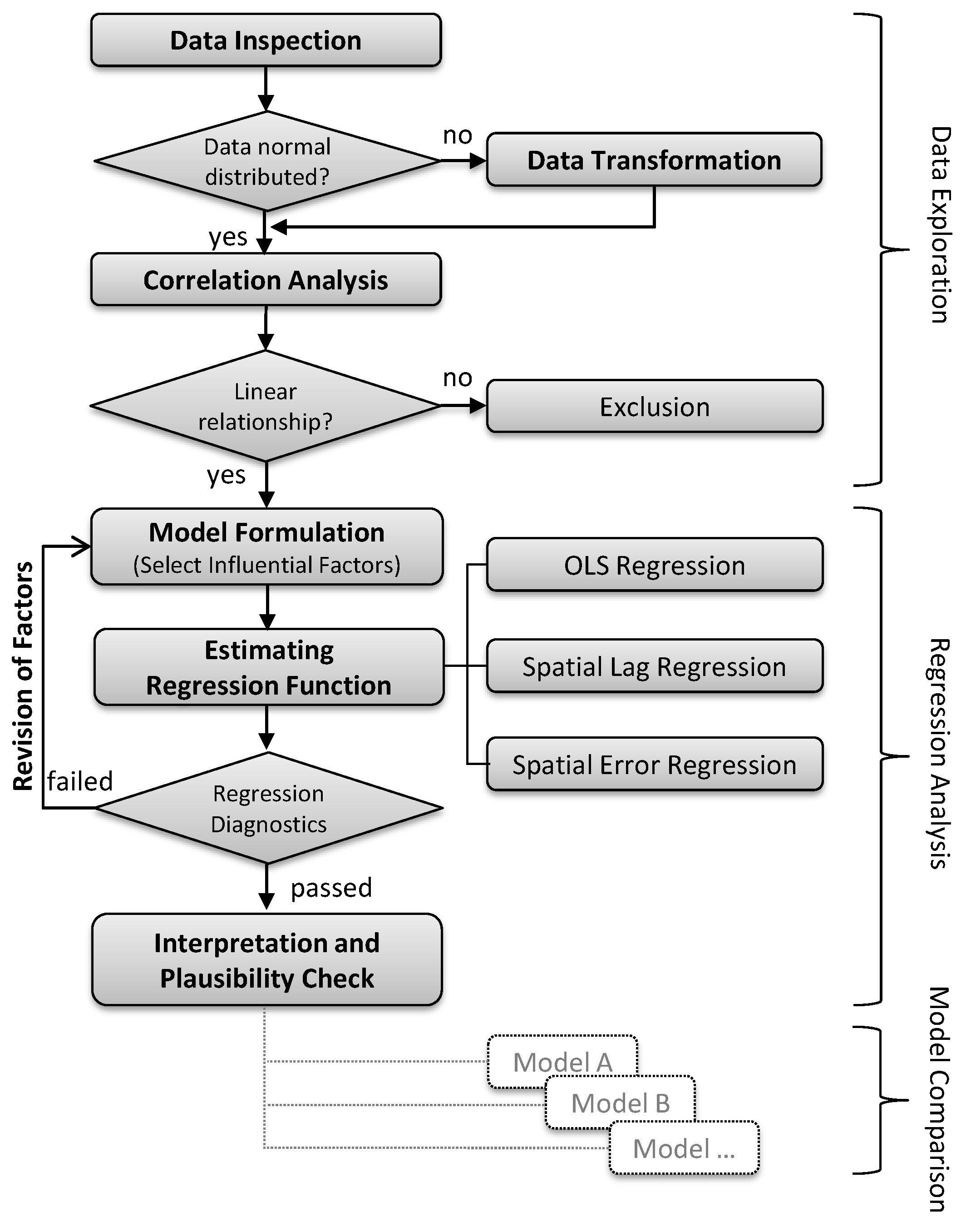
5. Methods
6. Results
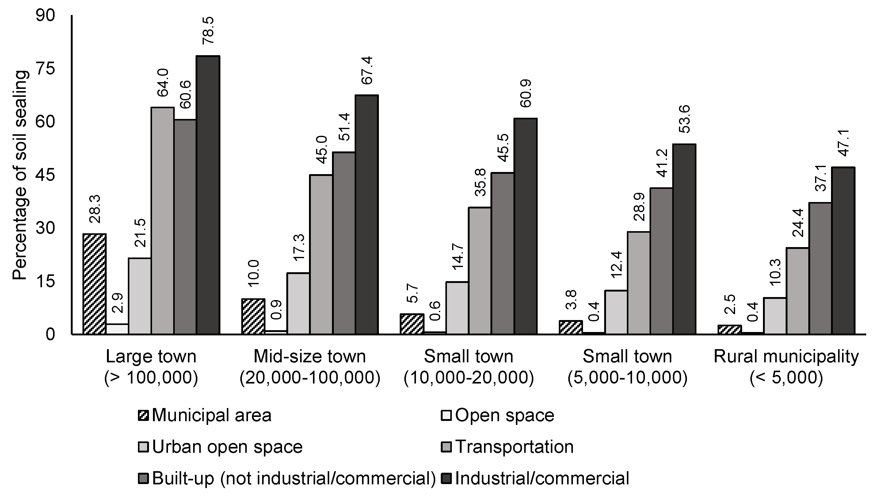
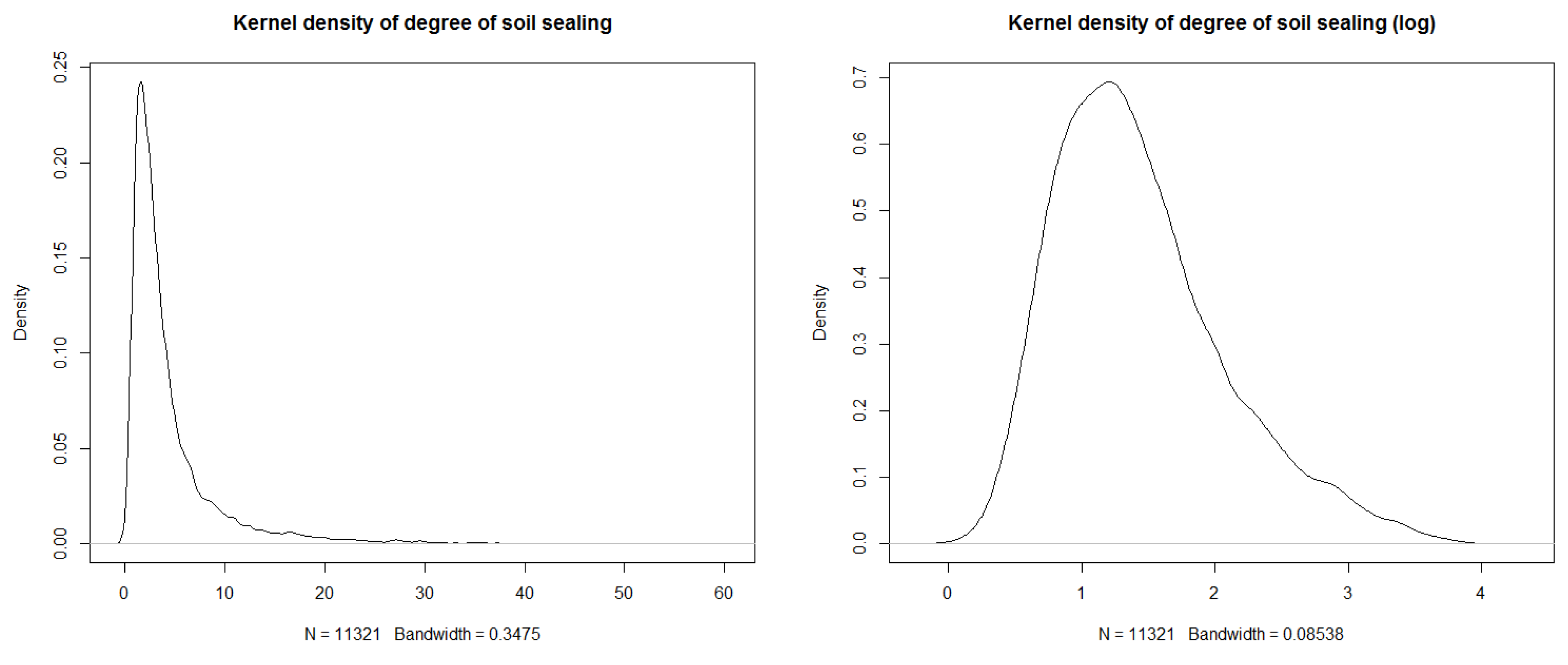
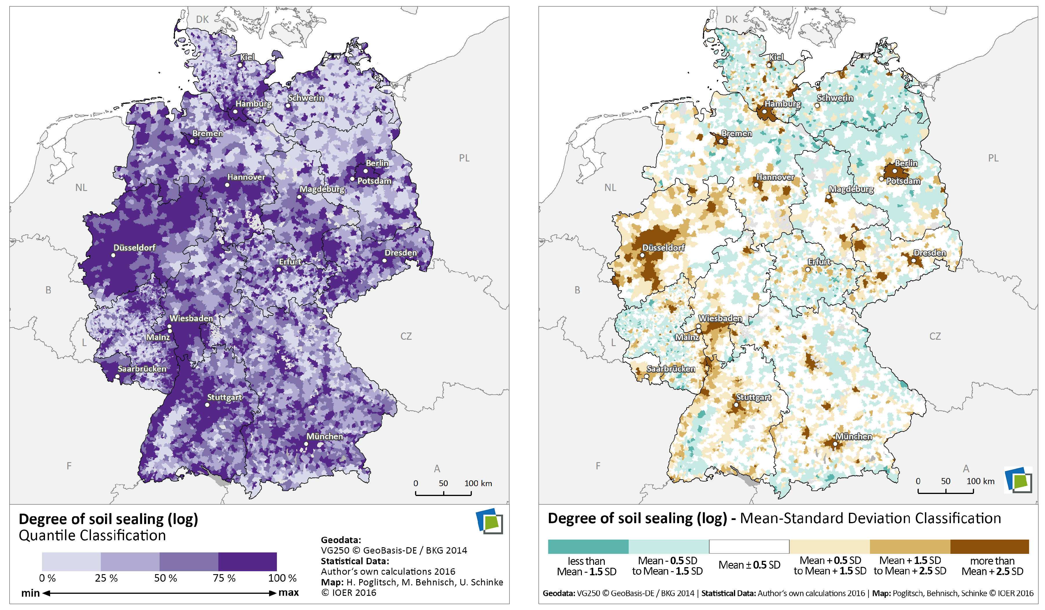
6.1. Data Inspection
6.2. Data Transformation
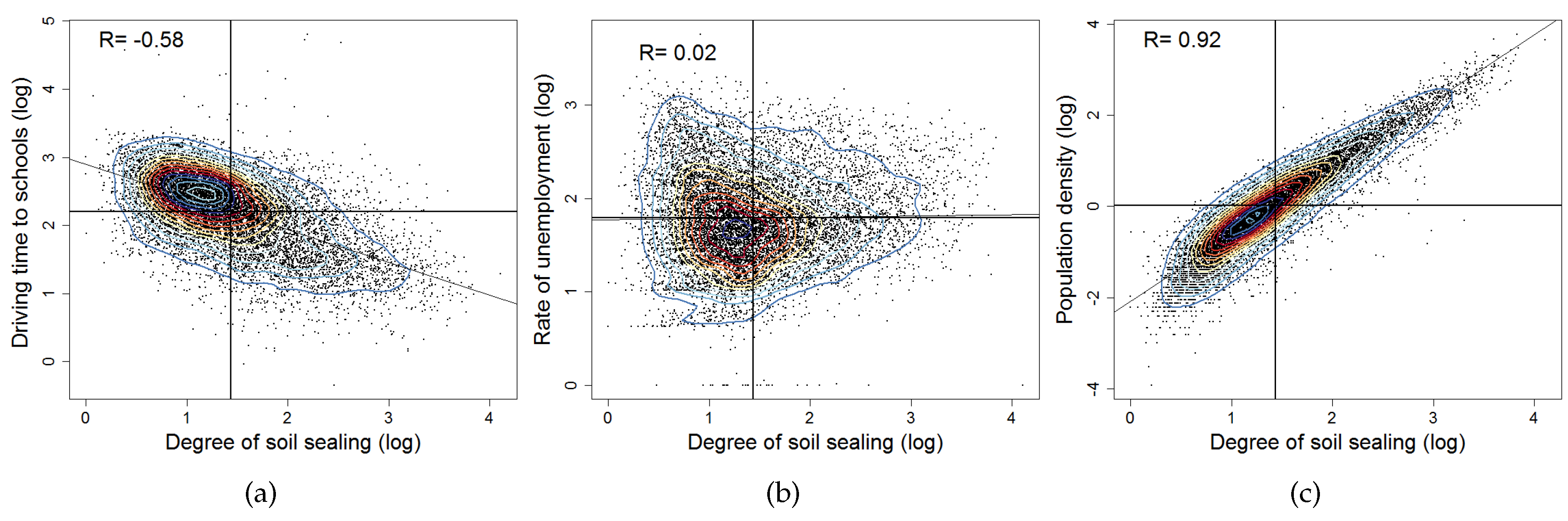
6.2.1. Correlation Analysis
6.2.2. Regression Analysis
6.2.3. Ordinary Least Squares Model
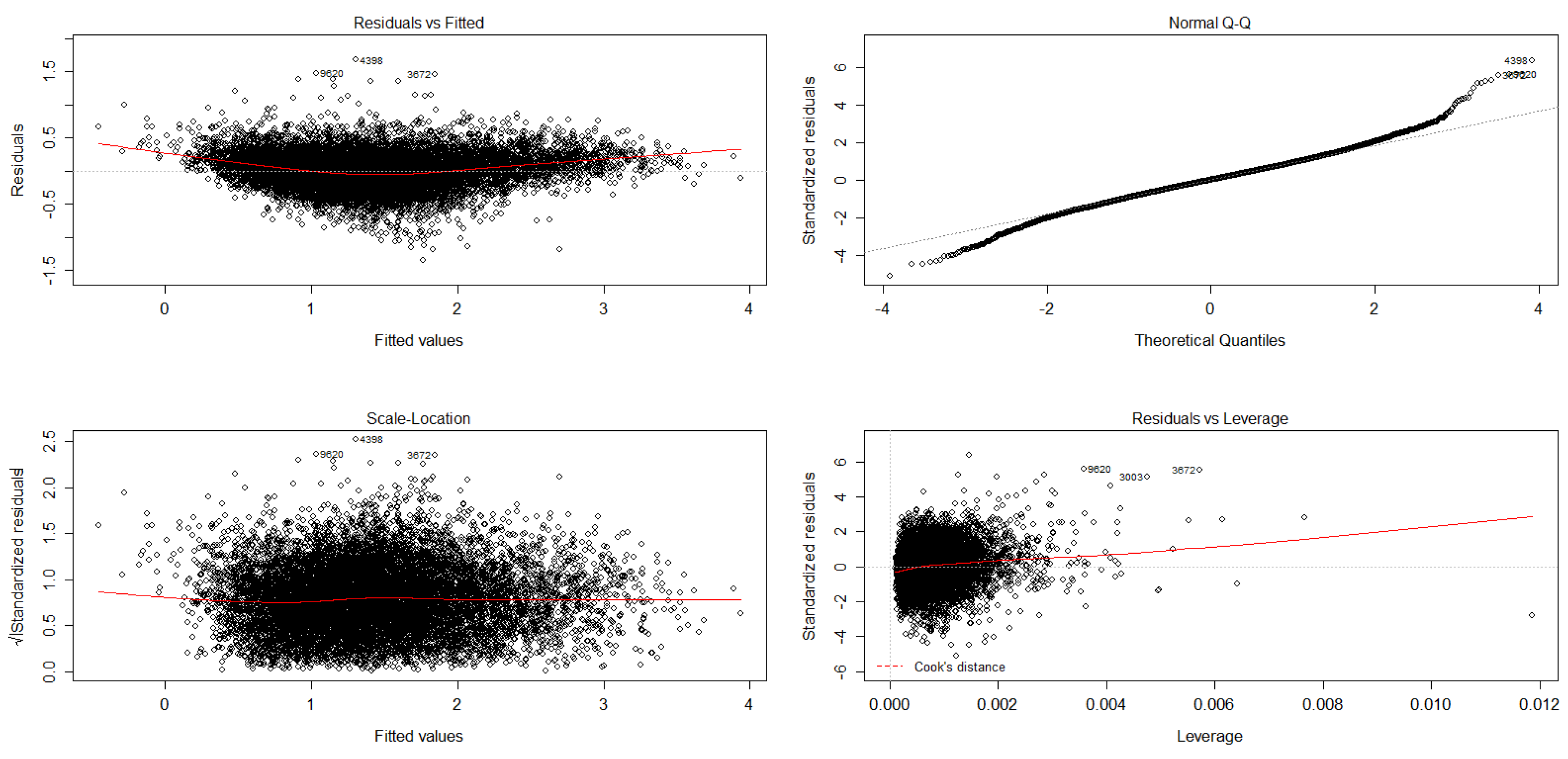
6.2.4. Regression Diagnostics
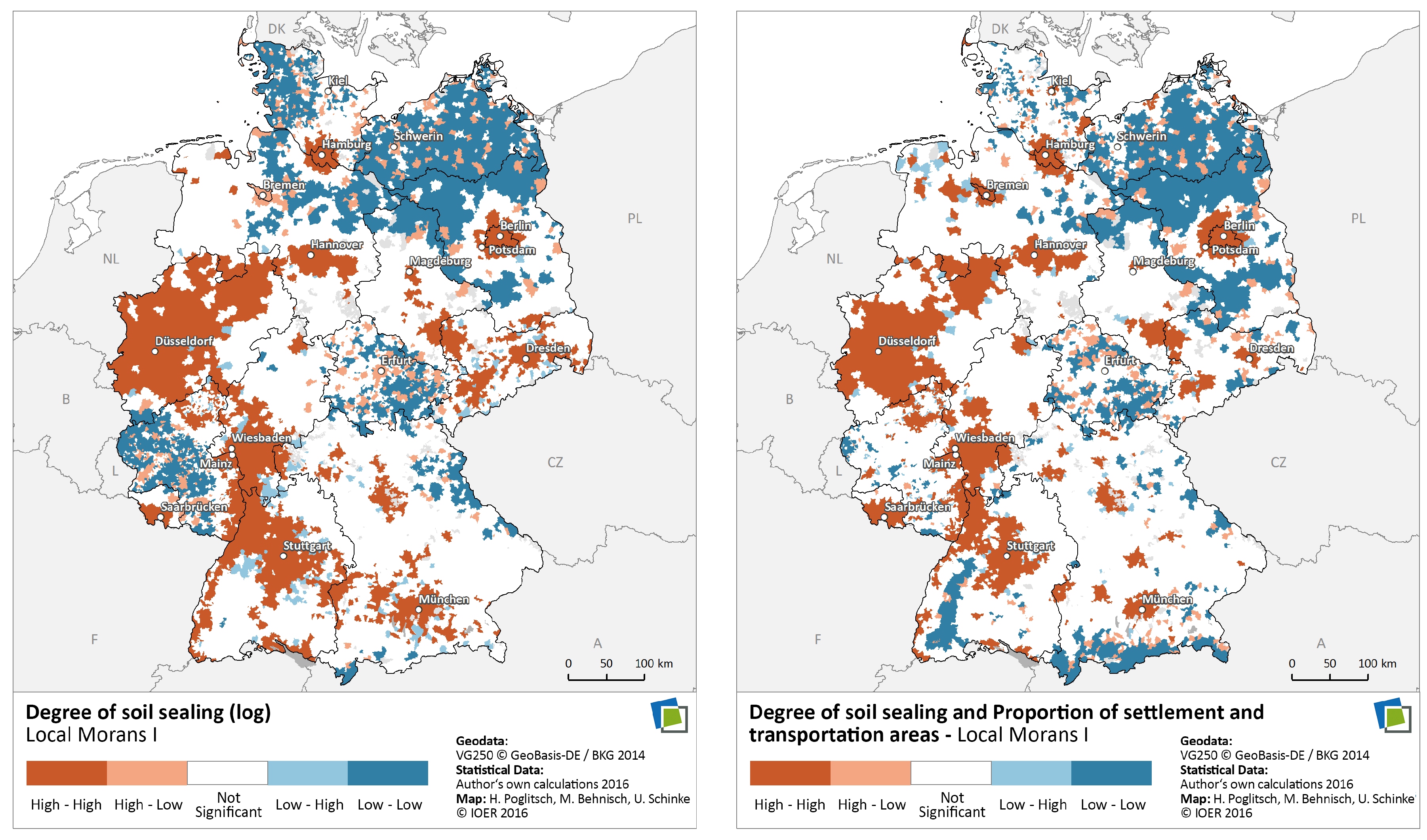
6.2.5. Spatial Regression Analysis
7. Discussion
8. Conclusions
Acknowledgments
Author Contributions
Conflicts of Interest
References
- Lexer, W. Zerschnitten, versiegelt, verbaut?—Flächenverbrauch und Zersiedelung versus nachhaltige Siedlungsentwicklung. In Fachtagung zur Stadtökologie “Grünstadtgrau”; Selbstverlag: Wien, Österreich, 2004; pp. 35–45. [Google Scholar]
- BMVBS/BBSR. Einflussfaktoren der Neuinanspruchnahme von Flächen; Forschungen Heft 139; BMVBS/BBSR: Bonn, Germany, 2009. [Google Scholar]
- Haber, W.; Bückman, W. Nachhaltiges Landmanagement, Differenzierte Landnutzung und Klimaschutz; Technische Universitätsverlag: Berlin, Germany, 2013. [Google Scholar]
- Siedentop, S.; Heiland, S.; Lehmann, I.; Hernig, A.; Schauerte-Lüke, N. Nachhaltigkeitsbarometer Fläche—Regionale Schlüsselindikatoren Nachhaltiger Flächennutzung für die Fortschrittsberichte der Nationalen Nachhaltigkeitsstrategie (Nachhaltigkeitsbarometer Fläche); Selbstverlag: Bonn, Germany, 2006. [Google Scholar]
- Haase, D.; Nuissl, H. Does urban sprawl drive changes in the water balance and policy? The case of leipzig (Germany) 1870–2003. Lands. Urban Plan. 2007, 80, 1–13. [Google Scholar] [CrossRef]
- Heber, B.; Lehmann, I. Beschreibung und Bewertung von Bodenversiegelung in Städten; Selbstverlag: Dresden, Germany, 1996. [Google Scholar]
- Lafortezza, R.; Carrusc, G.; Sanesia, G.; Davies, C. Benefits and well-being perceived by people visiting green spaces in periods of heat stress. Urban For. Urban Green. 2009, 8, 97–108. [Google Scholar] [CrossRef]
- Lassen, C. Unzerschnittene verkehrsarme Räume in der Bundesrepublik Deutschland. Nat. Landsch. 1979, 54, 333–334. [Google Scholar]
- Prokop, G.; Jobstmann, H.; Schönbauer, A. Overview of Best Practices for Limiting Soil Sealing or Mitigating its Effects in EU-27; Final Report of a study contracted by the European Commission, DG Environment; European Communities: Brussels, Belgium, 2011. [Google Scholar]
- Scalenghea, R.; Marsan, F.A. The anthropogenic sealing of soils in urban areas. Lands. Urban Plan. 2009, 90, 1–10. [Google Scholar] [CrossRef]
- Arlt, G.; Gössel, J.; Heber, B.; Hennersdorf, J.; Lehmann, I.; Thinh, N.X. Auswirkungen Städtischer Nutzungsstrukturen auf Bodenpreis und Bodenversiegelung; IÖR Schriften Band 34; Sächsiches Druck und Verlagshaus: Dresden, Germany, 2001. [Google Scholar]
- Martin, C.; Eiblmaier, M. (Eds.) Lexikon der Geowissenschaften; Spektrum Akademischer Verlag: Heidelberg, Germany, 2002.
- EEA, European Environmental Agency. Imperviousness products 2006/2009: Technical Note on HR Imperviousness Layer Product Specification; European Environmental Agency: Copenhagen, Denmark, 2010. [Google Scholar]
- Blum, W.E.H. Challenges for European soil protection under interdisciplinary aspects. In Europäischer Bodenschutz: Schlüsselfragen des nachhaltigen Bodenschutzes; Lee, Y.H., Bückmann, W., Eds.; Universitätsverlag: Berlin, Germany, 2008; pp. 81–94. [Google Scholar]
- Breuste, J.H. Structural analysis of urban landscapes for landscape management in German cities. In Ecology of Cities and Towns; McDonnell, M.J., Hahs, A.K., Breuste, J.H., Eds.; University Press: Cambridge, UK, 2009; pp. 355–379. [Google Scholar]
- Acevedo, W.; Taylor, J.L.; Hester, D.J.; Mladinich, C.S.; Glavac, S. Rates, Trends, Causes, and Consequences of Urban Land-Use Change in the United States; USGS Information Services: Denver, CO, USA, 2006; p. 70. [Google Scholar]
- Frie, B.; Hensel, R. Schätzverfahren zur Bodenversiegelung: UGRdL-Ansatz. In Statistische Analysen und Studien NRW, Band 44; Landesamt für Datenverarbeitung und Statistik NRW; Selbstverlag: Düsseldorf, Germany, 2007; pp. 19–32. [Google Scholar]
- Meinel, G.; Hernig, A. Erhebung der bodenversiegelung auf grundlage des ATKIS-Basis-DLM- möglichkeiten und grenzen. Photogramm. Fernerkund. Geoinform. 2006, 3, 195–204. [Google Scholar]
- Braun, M.; Herold, M. Mapping impervious surface using NDVI and linear spectral unmixing of ASTER data in the Cologne-Bonn region (Germany). SPIE Proc. 2004, 5239, 274–284. [Google Scholar]
- Kübler, A. Kommunale Bodenschutzkonzepte—Bewertung, Monitoring und Management von Bodenressourcen, Vorgestellt am Beispiel Stuttgart; Neue Möglichkeiten der Nachhaltigkeit im Kommunalen Bodenschutz durch Kombination von Bodenbewertung, Bodenindikatoren und Strategien zur Haushälterischen Bewirtschaftung Lokaler Bodenressourcen. Ph.D. Thesis, Universität Stuttgart, Stuttgart, Germany, 2004. [Google Scholar]
- Goetzke, R.; Over, M.; Braun, M. A method to map land-use change and urban growth in North Rhine-Westphalia (Germany). In Proceedings of the 2nd Workshop of the EARSeL SIG on Land Use and Land Cover, Bonn, Germany, 6–7 May 2006; pp. 102–111.
- Esch, T.; Himmler, V.; Schorcht, G.; Thiel, M.; Wehrmann, T.; Bachofer, F.; Conrad, C.; Schmidt, M.; Dech, S. Large-area assessment of impervious surface based on integrated analysis of single-date Landsat-7 images and geospatial vector data. Remote Sens. Environ. 2009, 113, 1678–1690. [Google Scholar] [CrossRef]
- Heldens, W.; Esch, T.; Heiden, U.; Dech, S.; Chockalingam, J. Potential of hyperspectral remote sensing for characterisation of urban structure in Munich. In Proceedings of the EARSeL Joint Workshop, Bochum, Germany, 5–7 March 2008; pp. 94–103.
- Wu, C.; Murray, A.T. Estimating impervious surface distribution by spectral analysis. Remote Sens. Environ. 2003, 84, 493–505. [Google Scholar] [CrossRef]
- Li, M.; Zang, S.; Wu, C.; Deng, Y. Segmentation-based and rule-based spectral mixture analysis for estimating urban imperviousness. Adv. Space Res. 2015, 55, 1307–1315. [Google Scholar] [CrossRef]
- Munafò, M.; Norerob, C.; Sabbic, A.; Salvati, L. Soil sealing in the growing city: A survey in Rome, Italy. Scott. Geogr. J. 2013, 126, 153–161. [Google Scholar] [CrossRef]
- Villa, P. Mapping urban growth using Soil and Vegetation Index and Landsat data: The Milan (Italy) city area case study. Landsc. Urban Plan. 2012, 107, 245–254. [Google Scholar] [CrossRef]
- Sunde, M.G.; He, H.S.; Zhou, B.; Hubbart, J.A.; Spicci, A. Imperviousness Change Analysis Tool (I-CAT) for simulating pixel-level urban growth. Landsc. Urban Plan. 2014, 124, 104–108. [Google Scholar] [CrossRef]
- Maucha, G.; Büttner, G.; Kosztra, B. European Validation of GMES FTS Soil Sealing Enhancement Data; Final draft; European Environment Agency: Copenhagen, Denmark, 2010. [Google Scholar]
- Maucha, G.; Büttner, G.; Kosztra, B. Europeanvalidation of GMES FTS soil sealing enhancement data. In Proceedings of the 31st EARSeL Symposium Prague: Remote Sensing and Geoinformation not only for Scientific Cooperation, Prague, Czech Republic, 30 May–2 June 2011; pp. 223–238.
- Ranalli, F.; Salvati, L. Complex patterns, unpredictable consequences: The distribution of sealed land along the urban-rural gradient in Barcelona. Documents d’Anàlisi Geogr. 2015, 61, 393–408. [Google Scholar] [CrossRef]
- Tombolini, I.; Munafòa, M.; Salvati, L. Soil sealing footprint as an indicator of dispersed urban growth: A multivariate statistics approach. Urban Res. Pract. 2015, 9, 1–15. [Google Scholar] [CrossRef]
- Artmann, M. Driving forces of urban soil sealing and constraints of ist management—Cases of leipzig and munich (Germany). J. Settl. Spat. Plan. 2013, 4, 143–152. [Google Scholar]
- Artmann, M. Spatial dimensions of soil sealing management in growing and shrinking cities—A systemic multiscale analysis in Germany. Erdkunde 2013, 67, 249–264. [Google Scholar] [CrossRef]
- Cabral, P.; Santos, J.; Augusto, G. Monitoring urban sprawl and the national ecological reserve in Sintra-Cascais, Portugal: Multiple OLS linear regression model evaluation. J. Urban Plan. Dev. 2011, 137, 346–353. [Google Scholar] [CrossRef]
- Mann, S. Was beeinflusst die flächenversiegelung? Agrarforschung 2008, 15, 184–189. [Google Scholar]
- Morelli, V.G.; Salvati, L. Ad Hoc Urban Sprawl in the Mediterranean City: Dispersing a Compact Tradition? Edizioni Nuova Cultura: Rom, Italy, 2010. [Google Scholar]
- Navarro Pedreño, J.; Meléndez-Pastor, I.; Gómez Lucas, I. Impact of three decades of urban growth on soil resources in Elche (Alicante, Spain). Span. J. Soil Sci. 2012, 2, 55–69. [Google Scholar]
- Vanderhaegen, S.; De Munter, K.; Canters, F. High resolution modelling and forecasting of soil sealing density at the regional scale. Landsc. Urban Plan. 2015, 133, 133–142. [Google Scholar] [CrossRef]
- Xiao, R.; Su, S.; Zhang, Z.; Qi, J.; Jiang, D.; Wu, J. Dynamics of soil sealing and soil landscape patterns under rapid urbanization. Catena 2013, 109, 1–12. [Google Scholar] [CrossRef]
- Thinh, N.X.; Arlt, G.; Heber, B.; Hennersdorf, J.; Lehmann, I. Evaluation of urban land-use structures with a view to sustainable development. Environ. Impact Assess. Rev. 2002, 22, 475–492. [Google Scholar] [CrossRef]
- Levia, D.F. Farmland conversion and residential development in North Central Massachusetts. Land Degrad. Dev. 1999, 9, 123–130. [Google Scholar] [CrossRef]
- Mann, S.; Zingg, E. Stand und Dynamik der Flächenversiegelung in der Schweiz. Raumforsch. Raumordn. 2009, 67, 45–53. [Google Scholar] [CrossRef]
- Kretschmer, O.; Ultsch, A.; Behnisch, M. Towards an understanding of land consumption in Germany—Outline of influential factors as a basis for multidimensional analyses. Erdkunde 2015, 69, 267–279. [Google Scholar] [CrossRef]
- Salvati, L.; Forino, G. A “laboratory” of landscape degradation: Social and economic implications for sustainable development in peri-urban areas. Int. J. Innov. Sustain. Dev. 2014, 8, 232–249. [Google Scholar] [CrossRef]
- Territorial Agenda of the European Union 2020: Towards an Inclusive, Smart and Sustainable Europe of Diverse Regions. Gödöllő, Hungary, 2011. Available online: http://www.eu2011.hu/files/bveu/documents/ TA2020.pdf (accessed on 15 April 2016).
- Müller, K.; Steinmeier, C.; Küchler, M. Urban growth along motorways in Switzerland. Landsc. Urban Plan. 2010, 98, 3–12. [Google Scholar] [CrossRef]
- EEA, European Environmental Agency. Urban Sprawl in Europe—The Ignored Challenge; European Environment Agency Report 10/2006; European Environmental Agency: Copenhagen, Denmark, 2006. [Google Scholar]
- Walz, U.; Stein, C. Indicators of hemeroby for the monitoring of landscapes in Germany. J. Nat. Conserv. 2014, 22, 279–289. [Google Scholar] [CrossRef]
- Bundesamt für Kartographie und Geodäsie (BKG, Federal Agency for Cartography and Geodesy). Available online: http://www.geodatenzentrum.de/docpdf/vg250.pdf (accessed on 10 June 2016).
- Behnisch, M.; Ultsch, A. Knowledge discovery in spatial planning data—A concept for cluster understanding. In Computational Approaches for Urban Environments; Geotechnologies and the Environment Series 13; Helbich, M., Arsanjani, J.J., Leitner, M., Gatrell, J.D., Jensen, R.R., Eds.; Springer: Berlin, Germany, 2015; pp. 49–75. [Google Scholar]
- Fox, J. Applied Regression Analysis, Linear Models, and Related Models; SAGE Publications: New York, NY, USA, 1997. [Google Scholar]
- Hand, D.J.; Mannila, H.; Smyth, P. Principles of Data Mining; The MIT Press: Cambridge, MA, USA, 2001. [Google Scholar]
- Ultsch, A. Pareto density estimation: A density estimation for knowledge discovery. In Innovations in Classification, Data Science, and Information Systems, Proceedings of the 27th Annual Conference of the German Classification Society (GfKL), Cottbus, Germany, 12–14 March 2003; Baier, D., Wernecke, K.D., Eds.; Springer: Berlin, Germany, 2003; pp. 91–100. [Google Scholar]
- Griffith, D.A. Spatial Autocorrelation; Elsevier Inc.: Dallas, Richardson, TX, USA, 2009. [Google Scholar]
- Longley, P.A.; Goodchild, M.F.; Maguire, D.J.; Rhind, D.W. Geographic Information Systems and Science; Wiley: New York, NY, USA, 2005. [Google Scholar]
- Anselin, L. Spatial Econometrics/Methods and Models; Springer Science & Business Media: Dodrecht, The Netherlands, 1988. [Google Scholar]
- Getis, A. Spatial autocorrelation. In Handbook of Applied Spatial Analysis; Fischer, M.M., Getis, A., Eds.; Springer: Berlin, Germany; pp. 255–278.
- Anselin, L. Local indicators of spatial association—LISA. Geogr. Anal. 1995, 27, 93–115. [Google Scholar] [CrossRef]
- Anselin, L.; Bera, A. Spatial Dependence in Linear Regression Models. In Handbook of Applied Economic Statistics; Marcel Dekker, Inc.: New York, NY, USA, 1998; pp. 237–289. [Google Scholar]
- Fischer, M.; Wang, J. Spatial Data Analysis/Models, Methods and Techniques; Springer: Heidelberg, Germany, 2011. [Google Scholar]
- Kissling, D.; Carl, G. Spatial autocorrelation and the selection of simultaneous autoregressive models. Glob. Ecol. Biogeogr. 2008, 17, 59–71. [Google Scholar] [CrossRef]
- Anselin, L. Lagrange multiplier test diagnostics for spatial dependence and spatial heterogeneity. Geogr. Anal. 1988, 20, 1–17. [Google Scholar] [CrossRef]
- Lloyd, C. Local Models for Spatial Analysis; CRC Press: Boca Raton, FL, USA, 2011. [Google Scholar]
- Behnisch, M. Urban Data Mining; KIT Scientific Publishing: Karlsruhe, Germany, 2008. [Google Scholar]
- Behnisch, M.; Ultsch, A. Urban data mining: Spatiotemporal exploration of multidimensional data. Build. Res. Inf. 2009, 37, 520–532. [Google Scholar] [CrossRef]
- Fotheringham, A.; Brunsdon, C.; Charlton, M. Geographically Weighted Regression: The Analysis of Spatially Varying Relationships; John Wiley & Sons Ltd.: New York, NY, USA, 2002. [Google Scholar]
- Brundson, C.; Charlton, M.E.; Harris, P. Living with Collinearity in Local Regression Models. Available online: http://www.geos.ed.ac.uk/ gisteac/proceedingsonline/GISRUK2012/Papers/presentation-9.pdf (accessed on 15 April 2016).
- Wheeler, D.; Tiefelsdorf, M. Multicollinearity and Correlation Among local Regression Coefficients in Geographically Weighted Regression; Springer: Berlin, Germany, 2005. [Google Scholar]
- Wheeler, D.; Paez, A. Geographically Weighted Regression. In Handbook of Applied Spatial Analysis; Fischer, M.M., Getis, A., Eds.; Springer: Berlin, Germany, 2010; pp. 461–486. [Google Scholar]
- Wheeler, D. Visualizing and diagnosing coefficients from Geographically Weighted Regression models. In Geospatial Analysis and Modelling of Urban Structure and Dynamics; Jiang, B., Yao, X., Eds.; Springer: Berlin, Germany, 2010; pp. 415–436. [Google Scholar]
- Wackernagel, H. Multivariate Geostatistics: An Introduction with Applications, 3rd ed.; Springer: Berlin, Germany, 2010. [Google Scholar]
- Krüger, T.; Meinel, G.; Schumacher, U. Land-use monitoring by topographic data analysis. Cartogr. Geogr. Inf. Sci. 2013, 40, 220–228. [Google Scholar] [CrossRef]


| Hypothesis | Dimension | Source |
|---|---|---|
| 1. Soil sealing is particularly high in densely-populated municipalities with/or areas showing high economic activity. It is observed that the migration of people and businesses from core settlement areas or from less attractive regions leads to high levels of vacant and derelict buildings, with underlying soils remaining sealed. | Demographic and social issues, economy | [2,11,31,40,45,46] |
| 2. Tourism infrastructure shows a very heterogeneous spatial dimension, indicating a weak correlation with soil sealing for the pan-German study. | Demographic and social issues | [36,46] |
| 3. The degree of soil sealing is higher for areas that enjoy good transport connections. The expansion of transport infrastructure closely determines the degree of soil sealing. | Mobility | [2,26,39,47] |
| 4. Municipalities with a surplus of inbound commuters presumably show an increased soil sealing in commercial and traffic areas, though this is not true of residential areas. | Mobility | [44] |
| 5. Soil sealing in commercial and settlement areas is driven by municipal revenues in the form of trade and income taxes. | Economy | [33] |
| 6. Lifestyles and consumption patterns (e.g., living space per household/inhabitant, journeys between home, work, shops and leisure areas) influence demand for new developments and, thus, are correlated with soil sealing. | Land and real estate market | [2,33,48] |
| 7. If a municipality has a large proportion of economic sectors with a low specific demand for land, then the degree of soil sealing will be smaller. | Land and real estate market | [2] |
| 8. The greater the influence of human activity on a landscape (reflecting the concept of hemeroby), the higher the degree of soil sealing. | Spatial context | [40,49] |
| 9. Natural features, such as topographical restrictions, can influence the spatial distribution of settlement areas/sealed surfaces. | Spatial context | [2,36] |
| 10. The degree of soil sealing largely depends on the category of land protection (regulation of land use by federal and regional planning authorities). Subsidies for urban reconstruction and rural development are provided to restrict the extent of soil sealing. | Politics | [2] |
| Dimension | Count | Examples | Data Sources |
|---|---|---|---|
| Demographic and Social Issues | 30 | Population Density, Gender Proportion, Births, Inward and Outward Migration, Migration Balance by Age Groups, Intensity of Tourism | Federal Institute for Research on Building, Urban Affairs and Spatial Development (BBSR), Regional Database Germany |
| Economy | 53 | Employees, Job Offers, Debts and New Debts, Tax Revenues per 1000 Inhabitants, Unemployment Rate | BBSR, Regional Database Germany, Federal Employment Agency |
| Land and Real Estate Market | 90 | Building Area, Residential Buildings and Dwellings, Living Space per Inhabitant, Dwelling Sizes, Age Groups of Residential Buildings, Newly-Constructed Buildings, Vacancy Rate, Household Size and Structure, Tenancy Ratio, Purchasing Power | IÖR Monitor, BBSR, Microm, Regional Database Germany |
| Mobility | 6 | Share of Daily Migration, Average Commuting Distance, Job Market Centrality | BBSR |
| Politics | 6 | Administrative Fragmentation, Funding per 1,000 Inhabitants (e.g., Urban Development Funding) | Federal Office for Economic Affairs and Export Control |
| Spatial Context | 36 | Travel Time by Car and Trucks to Selected Places (Highways, Regional Centers, Airports, etc.), Hemeroby, Relief Diversity, Road Network Density, Air Pollutants | IÖR Monitor, Federal Environmental Agency, BBSR, Federal Statistical Office |
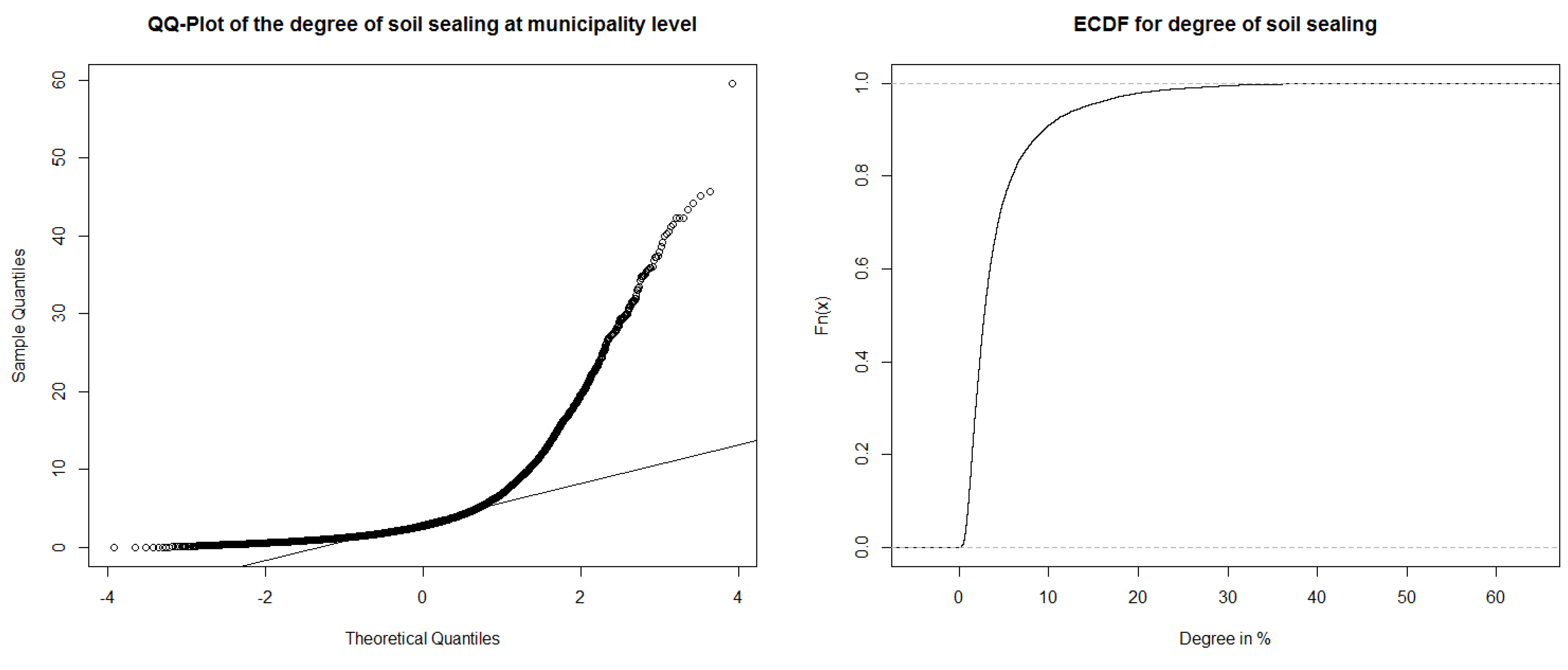
| Min | 1st Quantile | Median | Mean | 3rd Quantile | Max |
|---|---|---|---|---|---|
| 0.000 | 1.614 | 2.767 | 4.355 | 4.959 | 59.560 |
| Variable | Shortcut | Unit | Transform | Corr. |
|---|---|---|---|---|
| Demographic and social issues | ||||
| Population density | P-density | / | log | 0.92 |
| Population absolute | P-absolute | − | log | 0.70 |
| Percentage of vacation homes | Vacation homes | % | log | −0.29 |
| Economy | ||||
| Municipal tax capacity per inhabitant | Tax capacity | log | 0.72 | |
| Employees at the place-of-residence | Residence | − | log | 0.70 |
| Employees at the place-of-work | Work | − | log | 0.65 |
| Property Tax A per inhabitant | Property tax | log(d + 10) | 0.64 | |
| Percentage of employees at the place-of-work | Working employees | % | − | −0.55 |
| Income of trade tax per inhabitant | Trade tax | log | 0.50 | |
| Percentage of industrial and commercial area | IndCom | % | log | 0.54 |
| Spatial context | ||||
| Settlement and transportation area | land consumption | % | log | 0.90 |
| Road network density | Road density | km/km | log | 0.86 |
| Density of use of transport infrastructure | T-density | person/km | log | 0.79 |
| Settlement density | S-density | person/ha | log | 0.75 |
| Utilization Density | Utilization density | person/ha | log | 0.72 |
| Daytime population density | D-density | person/ha | log | 0.70 |
| Driving time to schools | Schools | minutes | log | −0.58 |
| Driving time to hospitals | Hospitals | minutes | log | −0.50 |
| Driving time to regional centers | Regional centers | minutes | log | −0.41 |
| Driving time to motorways | Motorways | minutes | log | −0.40 |
| Driving time by truck to cargo centers | Cargo centers | minutes | log | −0.40 |
| Land and real estate market | ||||
| Density of flats | F-density | % | log | 0.75 |
| Housing density | H-density | buildings/ha | log | 0.65 |
| Building area per 1000 inhabitant | building area | ha/inhabitant | log | 0.59 |
| Living space per inhabitant | Living space | m/inhabitant | log | 0.58 |
| Residential buildings per 1000 inhabitants | Buildings/inhab. | − | log | 0.58 |
| Percentage of multifamily houses | Buildings 3-X | % | log | 0.55 |
| Mobility | ||||
| Perc. of out-commuters | Out-commuters | % | 0.56 | |
| Job market centrality | Job centrality | % | log | 0.53 |
| Typical commuting distance | Commuting | km | − | −0.43 |
| Variable | Model A: Density | Variable | Model B: Driving Time | ||
|---|---|---|---|---|---|
| Beta | Stand. Beta | Beta | Stand. Beta | ||
| Intercept | −0.678 | ||||
| Intercept | −0.443 | Schools | −0.423 | −0.351 | |
| D-Density | −0.068 | 0.065 | Hospitals | −0.242 | −0.180 |
| F-Density | 0.085 | 0.264 | Regional Centers | −0.195 | −0.152 |
| Road Density | 1.195 | 0.640 | Motorways | −0.074 | −0.084 |
| Cargo Centers | −0.219 | −0.177 | |||
| 0.79 | 0.46 | ||||
| AIC | 4277.05 | AIC | 15188.50 | ||
| Variable | Model C: Influential Factors I | Variable | Model D: Influential Factors II | ||
| Beta | Stand. Beta | Beta | Stand. Beta | ||
| Intercept | 1.092 | Intercept | −0.678 | ||
| P-Density | 0.513 | 0.816 | Vacation Homes | −0.068 | −0.081 |
| Vacation Homes | −0.037 | −0.045 | Buildings 3-X | 0.075 | 0.091 |
| Buildings 3-X | 0.043 | 0.053 | Job Centrality | 0.040 | 0.093 |
| Job Centrality | 0.036 | 0.085 | Commuting | 0.003 | 0.028 |
| Commuting | 0.004 | 0.031 | S-Density | 0.185 | 0.171 |
| Schools | −0.023 | −0.019 | Road Density | 1.104 | 0.590 |
| Trade Tax | 0.031 | 0.061 | Tax Capacity | 0.044 | 0.120 |
| 0.86 | 0.83 | ||||
| AIC | −402.22 | AIC | 1907.54 | ||
| OLS Regression | Spatial Lag Regression | Spatial Error Regression | ||
|---|---|---|---|---|
| Model A | Pseudo- | 0.79 | 0.81 | 0.89 |
| AIC | 4277.05 | 3201.11 | −1165.53 | |
| Model B | Pseudo- | 0.46 | 0.57 | 0.61 |
| AIC | 15,188.50 | 13,128.4 | 12,301.5 | |
| Model C | Pseudo- | 0.86 | 0.87 | 0.92 |
| AIC | −402.22 | −750.01 | −4581.8 | |
| Model D | Pseudo- | 0.83 | 0.85 | 0.91 |
| AIC | 1907.54 | 1099.9 | −3344.02 |
© 2016 by the authors; licensee MDPI, Basel, Switzerland. This article is an open access article distributed under the terms and conditions of the Creative Commons Attribution (CC-BY) license (http://creativecommons.org/licenses/by/4.0/).
Share and Cite
Behnisch, M.; Poglitsch, H.; Krüger, T. Soil Sealing and the Complex Bundle of Influential Factors: Germany as a Case Study. ISPRS Int. J. Geo-Inf. 2016, 5, 132. https://doi.org/10.3390/ijgi5080132
Behnisch M, Poglitsch H, Krüger T. Soil Sealing and the Complex Bundle of Influential Factors: Germany as a Case Study. ISPRS International Journal of Geo-Information. 2016; 5(8):132. https://doi.org/10.3390/ijgi5080132
Chicago/Turabian StyleBehnisch, Martin, Hanna Poglitsch, and Tobias Krüger. 2016. "Soil Sealing and the Complex Bundle of Influential Factors: Germany as a Case Study" ISPRS International Journal of Geo-Information 5, no. 8: 132. https://doi.org/10.3390/ijgi5080132
APA StyleBehnisch, M., Poglitsch, H., & Krüger, T. (2016). Soil Sealing and the Complex Bundle of Influential Factors: Germany as a Case Study. ISPRS International Journal of Geo-Information, 5(8), 132. https://doi.org/10.3390/ijgi5080132