Density-Based Clustering with Geographical Background Constraints Using a Semantic Expression Model

Abstract

A semantics-based method for density-based clustering with constraints imposed by geographical background knowledge is proposed. In this paper, we apply an ontological approach to the DBSCAN (Density-Based Geospatial Clustering of Applications with Noise) algorithm in the form of knowledge representation for constraint clustering. When used in the process of clustering geographic information, semantic reasoning based on a defined ontology and its relationships is primarily intended to overcome the lack of knowledge of the relevant geospatial data. Better constraints on the geographical knowledge yield more reasonable clustering results. This article uses an ontology to describe the four types of semantic constraints for geographical backgrounds: “No Constraints”, “Constraints”, “Cannot-Link Constraints”, and “Must-Link Constraints”. This paper also reports the implementation of a prototype clustering program. Based on the proposed approach, DBSCAN can be applied with both obstacle and non-obstacle constraints as a semi-supervised clustering algorithm and the clustering results are displayed on a digital map.

1. Introduction

The importance of semantics in GIS (Geographic Information Systems) has been drawing an increasing amount of attention in the context of various applications, such as geographic data integration, data retrieval, way-finding systems, and geographic knowledge discovery. Geospatial clustering, which improves on standard clustering algorithms by incorporating background knowledge, cannot be explicitly excluded in GIS applications. Such clustering must depend on prior GIS domain knowledge and the context of the GIS user. Making better use of geospatial and clustering knowledge to select suitable constraints and parameters is likely to yield better and more meaningful clusters.

Geospatial data mining [1] is the extraction of implicit knowledge, geospatial relations, and interesting characteristics and patterns that are not explicitly represented in a geospatial database. Currently, the main application of geospatial data mining is to analyze geographic data with the intent of extracting and transmitting geospatial information. Geospatial analysis is the essence of GIS, enabling hidden information and knowledge to be obtained from geographic data. Geospatial data mining can be used in cartography and surveying, but it is not limited to these fields.

Geospatial clustering is an important area of research in geospatial data mining. Clustering algorithms play a key role in GIS spatial analysis techniques such as polygon overlay [2]. There is a need for practical solutions in a variety of constrained clustering applications. To improve the usefulness of clustering, therefore, it is vital to study constraint-based geospatial clustering analysis. The concept of introducing an approach based on the geospatial background into the geospatial problem-solving process is not new, as evidenced by numerous works. In particular, geospatial semantic graphs have been applied for the representation and analysis of remote sensing data [3]. Moreover, several other studies have addressed constraints on clustering [4,5,6], but these have often ignored semantic constraints; especially little attention has been paid to the semantics of geographical constraints.

The well-known DBSCAN (Density-Based Geospatial Clustering of Applications with Noise) [7] clustering algorithm has several deficiencies. In particular, there is a lack of geographical background knowledge (geospatial clustering constraints), and significant difficulties are encountered in acquiring and representing the relationships among geospatial knowledge. Most of the existing clustering methods focus solely on the data themselves, without considering constraining factors (such as different cities, river obstacles and mountain obstacles, etc.). Thus, clustering is performed at the data level instead of at the knowledge level, which prevents users from fully understanding the clustering results. Despite this, there have been few studies on domain knowledge-based clustering with constraints. Developments in the field of knowledge engineering, including ontology engineering, have vastly improved our ability to model data and infer relationships. However, the method has many shortcomings in supporting the use of geographical background knowledge for the formulation of constraints. Ruiz et al. developed the C-DBSCAN (density-Based clustering with constraints) [8] method, which offers improved performance over DBSCAN with a small number of constraints. However, C-DBSCAN cannot handle real geographical constraints, and is lack of semantics.

In order to solve above problems, this paper proposes a new method, which is based on geographical background knowledge. DBSCAN Ontology (DBSCANO) has been developed in accordance with the DBSCAN process and geographic information data characteristics. The C-DBSCANO algorithm has been realized by introducing DBSCANO to DBSCAN. It makes that the operation process of clustering in DBSCAN under the constraints of geographical background semantic knowledge and the clustering results are found to be more reasonable.

To solve these problems, this paper proposes a new method of exploiting geographical background knowledge. DBSCAN Ontology (DBSCANO) was developed to be compatible with the DBSCAN process and geographic data characteristics. The C-DBSCANO algorithm was developed by combining DBSCANO with DBSCAN. These tools enable clustering in DBSCAN under constraints based on geographical background semantic knowledge, leading to more reasonable clustering results.

The remainder of the paper is organized as follows. Section 2 introduces previous studies of geospatial clustering and ontologies. Section 3 describes the framework for DBSCAN with an ontology. Section 4 describes a reasoner based on dotNetRDF. Section 5 describes the results obtained using an implementation of the C-DBSCANO algorithm. We present the conclusions and discuss potential future studies in Section 6.

2. Previous Work: Geospatial Clustering and Ontologies

2.1. DBSCAN

DBSCAN uses the spatial density of an object’s class connectivity to quickly determine aggregated shape classes. The basic idea is that each object has a class and is contained in its domain within some minimum radius. Clustering algorithms can be broadly categorized as either hierarchical or partitioning [9]. Depending on one’s definition of a cluster, each category can be further classified as a distance-based, model-based, or density-based method, and density-based clustering can use either a grid-based or a neighborhood-based strategy [10]. The DBSCAN algorithm is a neighborhood-based strategy for density-based partitioning.

In most practical cases, the results of geospatial data mining must be applied when solving a clustering problem under various constraints to improve the usefulness of the clustering. Carlos Ruiz et al. [10] developed density-based semi-supervised clustering of data points to obtain the new algorithm C-DBSCAN. C-DBSCAN exhibits improved performance compared with DBSCAN even with a small number of constraints. C-DBSCAN introduces the concept of “Cannot-Link” (according to the background knowledge, the two objects must be directly classified as the same cluster) and “Must-Link” (according to the background knowledge, the two objects cannot be directly classified as the same cluster) constraints into DBSCAN. However, the method has no real geographical constraints. Moreover, C-DBSCAN has the side effect of generating many singleton clusters. The C-DBSCAN framework has little regard for the context semantics of the constraints that are relevant to GIS data in real geographical environments, which often leads to analysis results that are inconsistent with the actual situation. C-DBSCAN can be said to rely on hard constraints rather than semantic constraints of geographical background.

In all, the DBSCAN algorithm and DBSCAN algorithm and C-DBSCAN algorithm are rarely considered in constraints of real geographic environment. Several examples of problematic clustering models are provided below.

1. The expression of the clustering constraints is limited, resulting in clustering that could incorrectly represent relationships in some scenarios.

The example depicted in Figure 1 shows a clustering result that could not be reasonable in some scenarios. The clustering result ignores the district boundaries because the clustering was performed entirely based on geometric criteria. If the district membership is important, as in school allocation problems, for example, then a corresponding constraint is needed. In the absence of any constraints based on administrative regions, points of interest from different administrative regions are clustered based purely on their proximity.

2. Eps and MinPts are inflexible and unreasonable, resulting in inappropriate clustering.

An example of clustering results obtained in such a case is shown in Figure 2.

In the above example, Eps (a parameter of distance) and MinPts (a parameter of the minimum cluster size) were set based on a single type of region: the Eps1 and MinPts1 parameters are well suited to urban regions but are not appropriate for regions with more dispersed settlement. However, both urban and suburban regions exist in this area. Therefore, when analyzing the suburbs, Eps and MinPts should be adjusted accordingly to obtain better clustering results.

As we have mentioned, traditional geospatial clustering algorithms tend to differ from those applied in actual applications, because problems specific to the spatial environment are often encountered. For example, consider a business group preparing to expand their operations in Wuhan (Hubei Province, central China) by building a number of supermarkets. The rational decision-making department wishes to establish shops in locations that are central to their customers’ residential addresses. In Wuhan, however, the environment is subject to geographical constraints, such as the Yangtze River and the Hanjiang River, as shown in Figure 3a. If these constraints are ignored, then geospatial data mining will result in the clusters shown in Figure 3b. These are clearly suboptimal because these clusters ignore the need for certain customers to travel long distances to cross the rivers. Therefore, this analysis is unreasonable in the scenario. The clustering results obtained when the river constraints are considered are shown in Figure 3c. It is thus apparent that for practical applications, DBSCAN should consider obstacle constraints. When used in the process of geospatial clustering, geographical background constraints are primarily intended to overcome the lack of knowledge of the relevant geospatial data.

After considering the above problems, we have determined that the constraints on the algorithm parameters (as shown in Figure 2) and the constraints on the spatial data (as shown in Figure 1) should both be described by our ontology in the context of DBSCAN.

2.2. Ontology

One of the most highly cited definitions of the term “ontology” was introduced by Gruber [11]: “An ontology is a formal, explicit specification of a shared conceptualization”. The purpose of an ontology is to capture knowledge that provides a common set of concepts and axioms for reasoning in related fields. For density-based clustering, an appropriate geographical background knowledge ontology is constructed of a variety of concepts and relations concerning geospatial characteristics and clustering.

Semantic issues exist that are related to the creation, use, and discussion of geographic information. When solving a geospatial clustering problem, users may collect geospatial data and background knowledge using a variety of methods and from a variety of sources. When the semantics of the data are not suitably captured throughout the process of geospatial analysis, the geo-data and analysis results may be misunderstood and used inappropriately. The main purpose of this paper is not to define overall concepts and relations for all geospatial analyses; instead, it presents an ontology specifically for the DBSCAN algorithm. We do this to mitigate the difficulties encountered in defining geographic semantics.

3. Framework for DBSCAN with an Ontology

Based on the DBSCAN algorithm, this paper introduces an ontology for geospatial semantic constraint relations and enriches this ontology using semantic representations of multiple geospatial distance measurements for cluster analysis in the geospatial data domain. The choice of geospatial semantic constraints is motivated by the importance of structural information in the DBSCAN interpretation of datasets with such constraints and by the intrinsic nature of most multi-geospatial distance semantics. In this paper, we focus on constraints related to ontology-based rules.

3.1. DBSCAN Ontology Structure

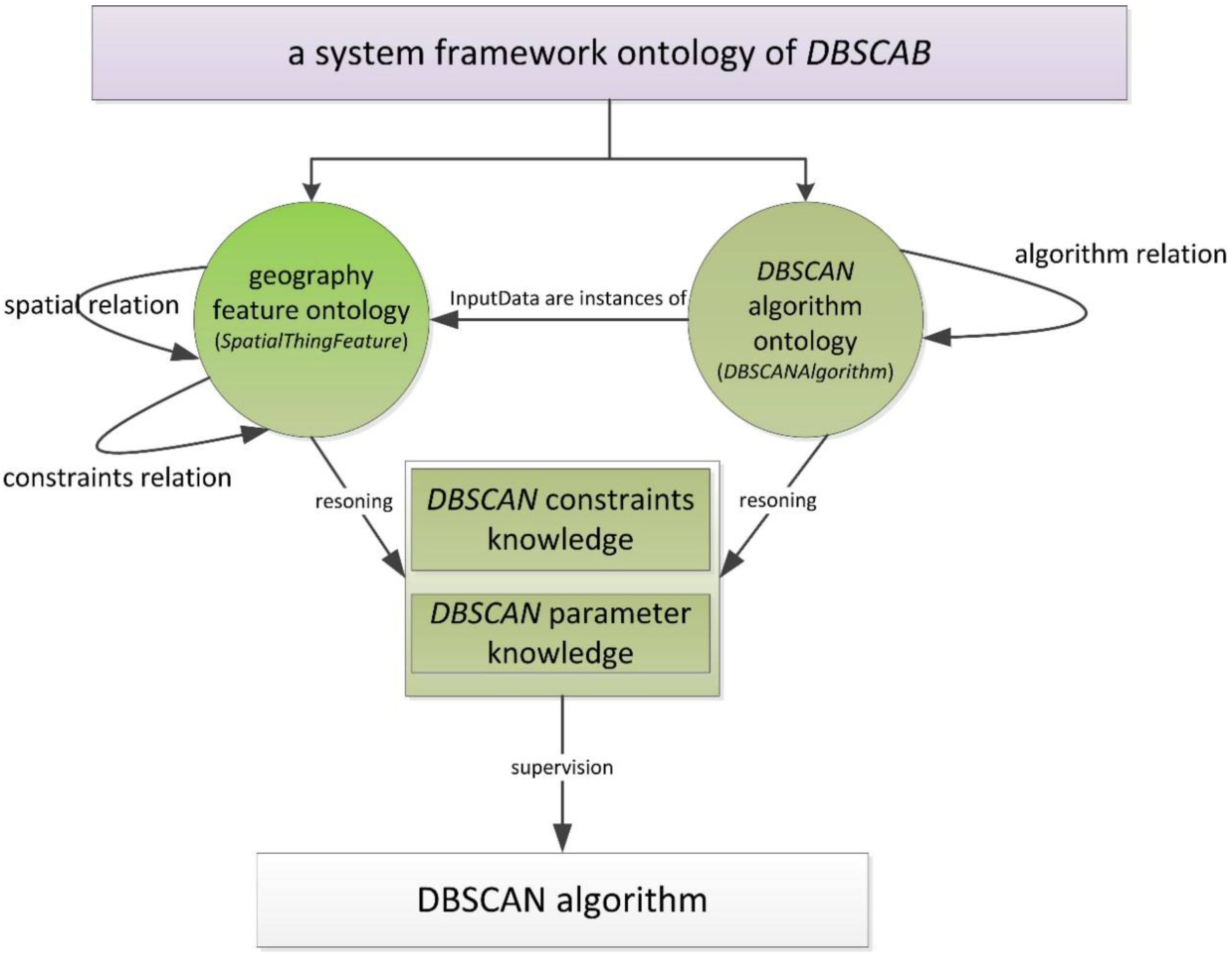
Ontologies, as a form of knowledge representation, have been used in various applications of geographic information. An application ontology in the DBSCAN domain can thus be regarded as a well-formed representation of clustering knowledge. Regarding the representation of the DBSCAN algorithm, the ontology includes knowledge of geospatial features, geospatial relations, and the DBSCAN algorithm itself. We can consider this knowledge to form a set of classes.

In this paper, we present the operational semantics to express this ontology using Notation3 (N3), as a 4-tuple O = <C, R, P, I>, where C is the set of concepts, R is the set of relations, I is the set of instances, and P is a set of properties that describe C. The DBSCAN ontology is developed to express the semantic knowledge of DBSCAN.

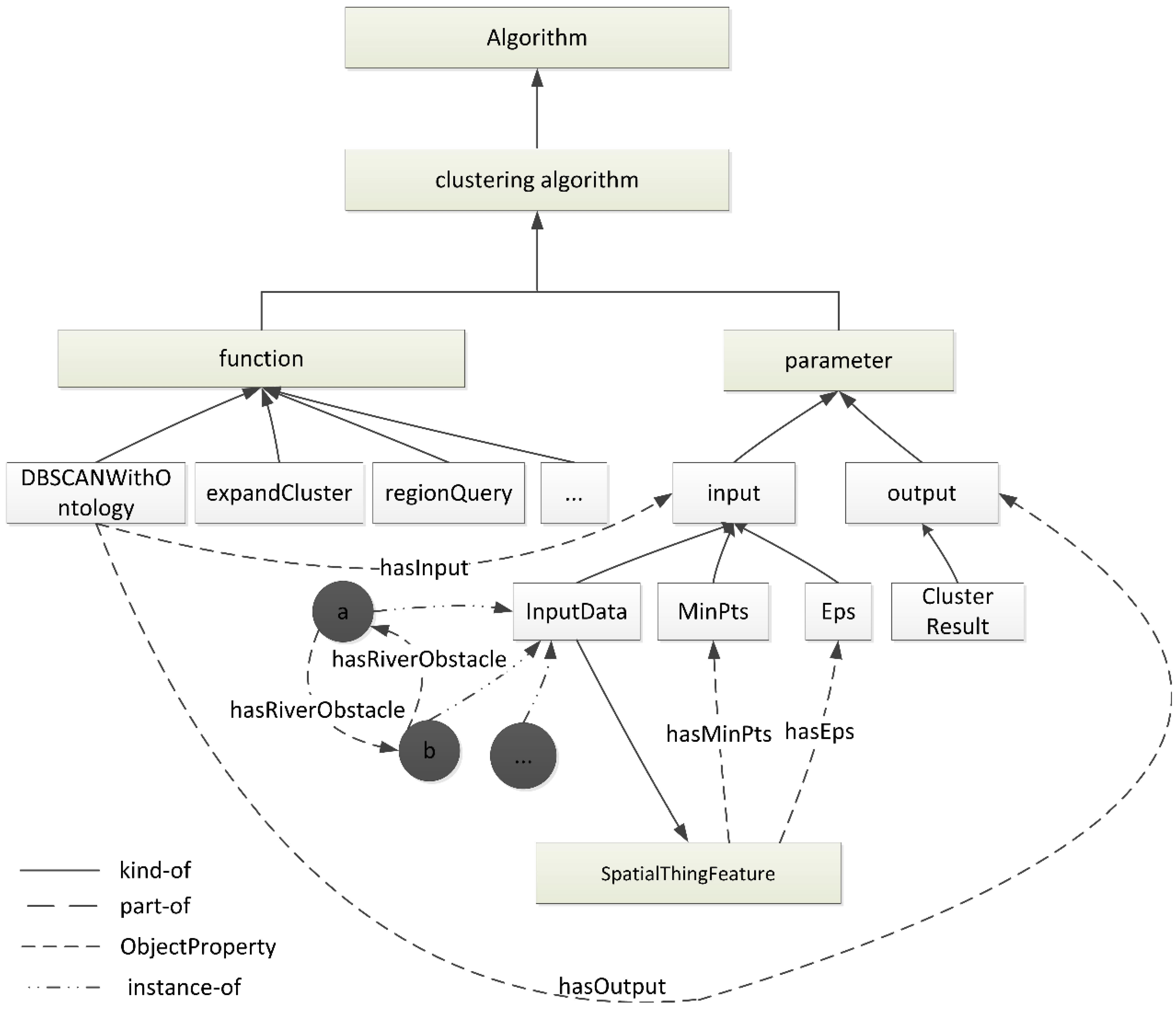
Example 1. Let us consider a simplified example ontology for DBSCAN. The domain identifier is DBSCANOntology. There are four concepts (GeospatialFeature, BaseFeature, POIFeature, and DBSCANAlgorithm) and four types of relations (distance, direction, topological, and constraint). The attribute set P is {Belong, Location, hasInput, hasOutput, IsReferenceFeature, DataType}, and the set of instances I is {ATM1, bankA, river1, scale1, eps1, …}.

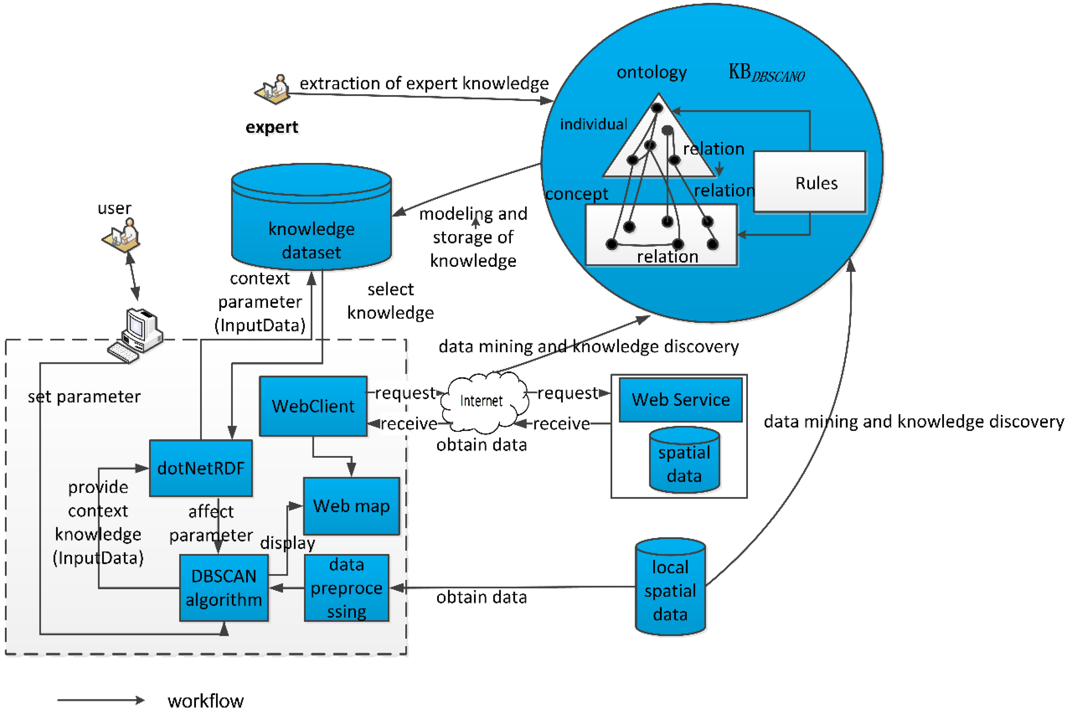
The geospatial relations are important in the application ontology of DBSCAN. The framework of DBSCAN with this ontology is illustrated in Figure 4.

3.2. Description of the DBSCAN Ontology

We have designed DBSCAN ontology that we call DBSCANO. This is an application-specific ontology for DBSCAN. The ontology includes knowledge of geospatial features and the DBSCAN algorithm. DBSCANO can be applied to the DBSCAN algorithm as introduced above. The purpose of introducing DBSCANO is to illustrate how the modeling decisions that are made in the framework are related to the ontologies.

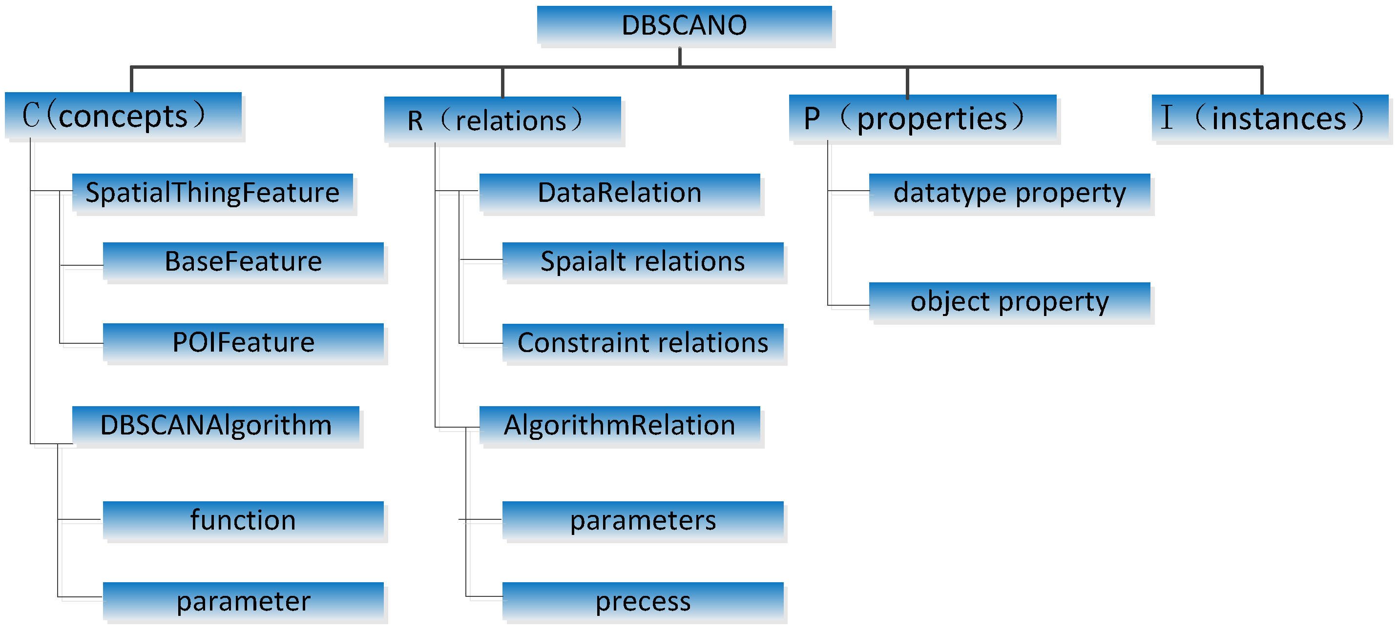
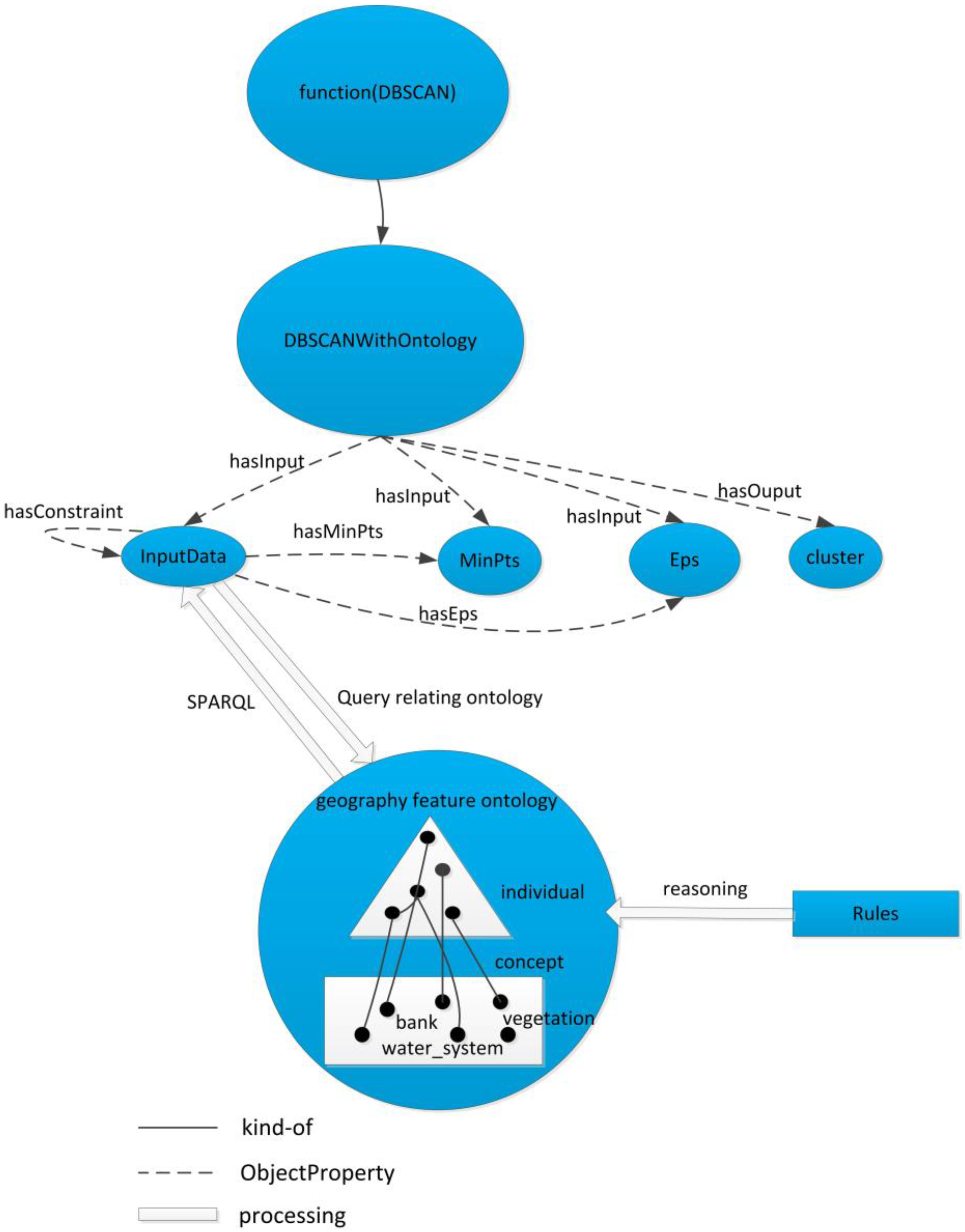
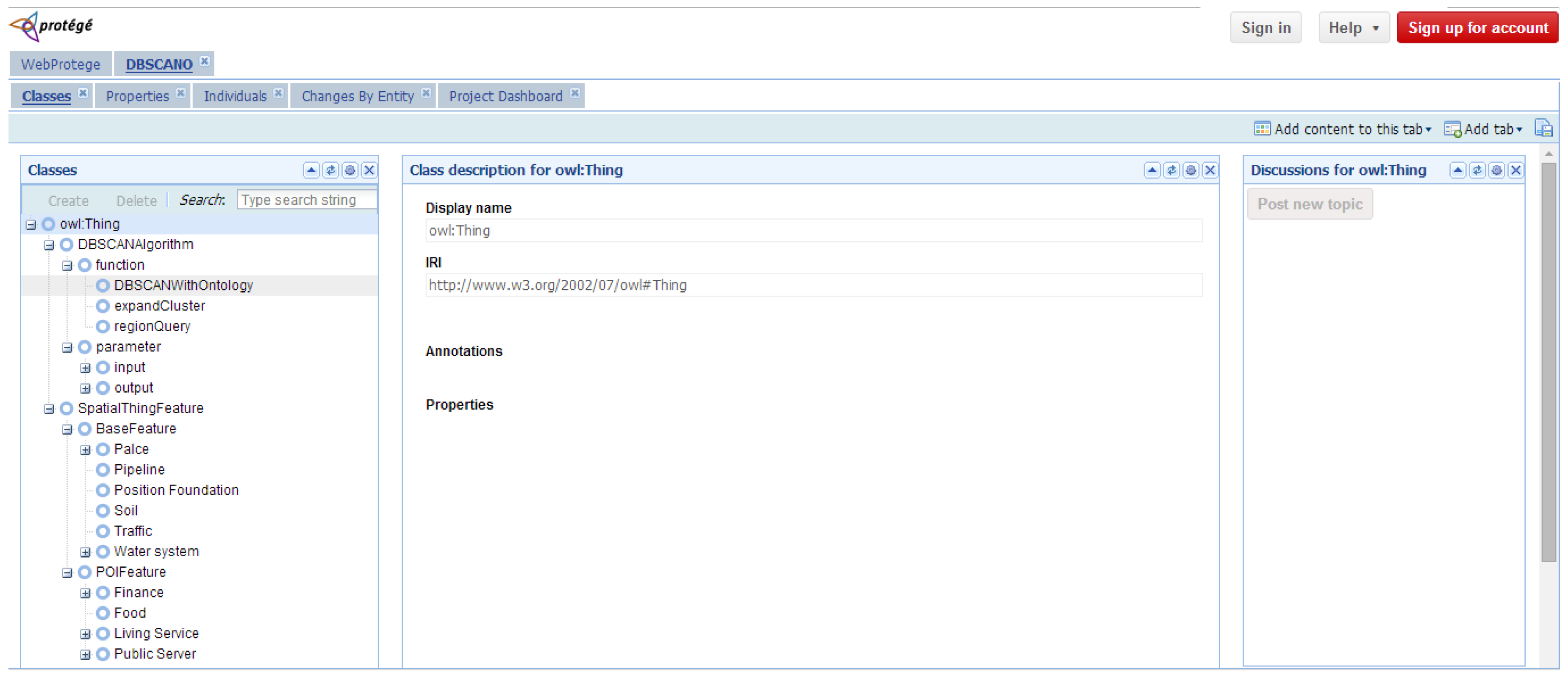
In this paper, we use the top-down method to construct DBSCANO. Firstly we analyze that the DBSCAN consists of spatial data and algorithm, then establish the conceptual system of spatial data and algorithms respectively, afterwards expand the ontology structure and establish the relationship between the data and the algorithm. The Structural of DBSCANO is illustrated in Figure 5. The Snapshot of part of hierarchy of DBSCANO in WebProtégé is illustrated in Figure 6 (http://webprotege.stanford.edu/#Edit:projectId=bbfed2b3-fb75-4cec-8148-6f798c86619f. Accessed 20 April 2016).

We now discuss each component of DBSCANO in detail.

(1) The set of concepts C includes two main classes, SpatialThingFeature and DBSCANAlgorithm.

SpatialThingFeature is a top-level class for geographic information objects. Its descendant classes serve to illustrate the concepts or objects related to geographic information objects in DBSCANO. Any feature or record of a dataset used in DBSCAN is an instance of SpatialThingFeature.

DBSCANAlgorithm represents the set of available DBSCAN clustering methods and the features of their interfaces. It is a core class of DBSCANO. DBSCANAlgorithm is related to SpatialThingFeature via DBSCAN relations. For example, DBSCANAlgorithm is related to SpatialThingFeature through a combination of the “instance-of” and “part-of” relationships. The features of DBSCANAlgorithm include the parameters required for DBSCAN, such as “Eps” and “MinPts”. The InputDataclass represents the input parameters for the POI data set in DBSCAN. An instance of the InputData class is related to SpatialThingFeature through the “type” property.

(2) The set R consists of relations between the above two classes, including DataRelation and AlgorithmRelation.

DataRelation defines the geospatial relations among instances of SpatialThingFeature. DataRelation objects are divided into two types: “spatial relations” and “constraint relations”. Spatial relations have been investigated in previous research [12]. DBSCANO includes three basic types of spatial relations: direction relations, distance relations, and topological relations. These were selected and expanded upon because their capacity for expressing spatial relations is well understood. A constraint relation is a key type of relation in DBSCANO. A constraint relation describes the logic underlying the limitations or stipulations that exist among geospatial objects of DBSCANO. Constraint relations may involve different districts and/or obstacles, and these relations include all possible DBSCAN constraints and user-generated sub-constraints, such as ConstraintsOfRiver and ConstraintsOfDifferentCity.

AlgorithmRelation defines effect relations among instances of DBSCANAlgorithm. In DBSCANO, an interaction relation describes the control of DBSCANAlgorithm or a change in its parameters. Examples of these effect relations are “Eps” and “MinPts”, which are selected through the “hasChangeWith” property of InputData. In DBSCANO, DBSCANRelation relations may facilitate reasoning to acquire parameter constraints for DBSCAN.

In DBSCANO, we can define the relations between properties of objects expressed using SpatialThingFeature, which are deduced based on the ontology for geographical background knowledge. The consistency of the relations contained in DBSCANO can be assessed. For example, there is a contrary relationship between “contain” and “belong” relations. The definition of these relations enables reasoning regarding certain constraints in DBSCANO. For example, left and right are inverse direction relations. If a fact in the ontology states that object a is to the left of object m (a mountain), then a constraint can be inferred through reasoning when a fact stating that object b is to the right of m is added to the ontology.

(3) The set P defines the attribute properties of the above classes and their sub-classes. In DBSCANO, a property is represented as a 2-tuple relation based on SpatialThingFeature and DBSCANAlgorithm. A property is a data literal or links to another instance. The attributes of SpatialThingFeature and DBSCANAlgorithm and the attributes that link them represent two major types of properties (data and algorithm properties). These attributes represent interconnections between SpatialThingFeature and DBSCANAlgorithm as defined in SpatialThingFeature and DBSCANAlgorithm. For example, the attributes of an instance of the “suburb” sub-class of SpatialThingFeature include hasEps (object property). The attributes of an instance of the InputDatasub-class of DBSCANAlgorithm include type (object property). An instance of the InputDatasub-class of DBSCANAlgorithm is related to a corresponding sub-class of SpatialThingFeature through a combination of the “type” and “subClassOf” relationships.

(4) The set I defines objects of SpatialThingFeature and DBSCANAlgorithm. These correspond to individual description logics. For instance, {Yangtze, Amazon, Thames…} is a set of “river” instances in DBSCANO.

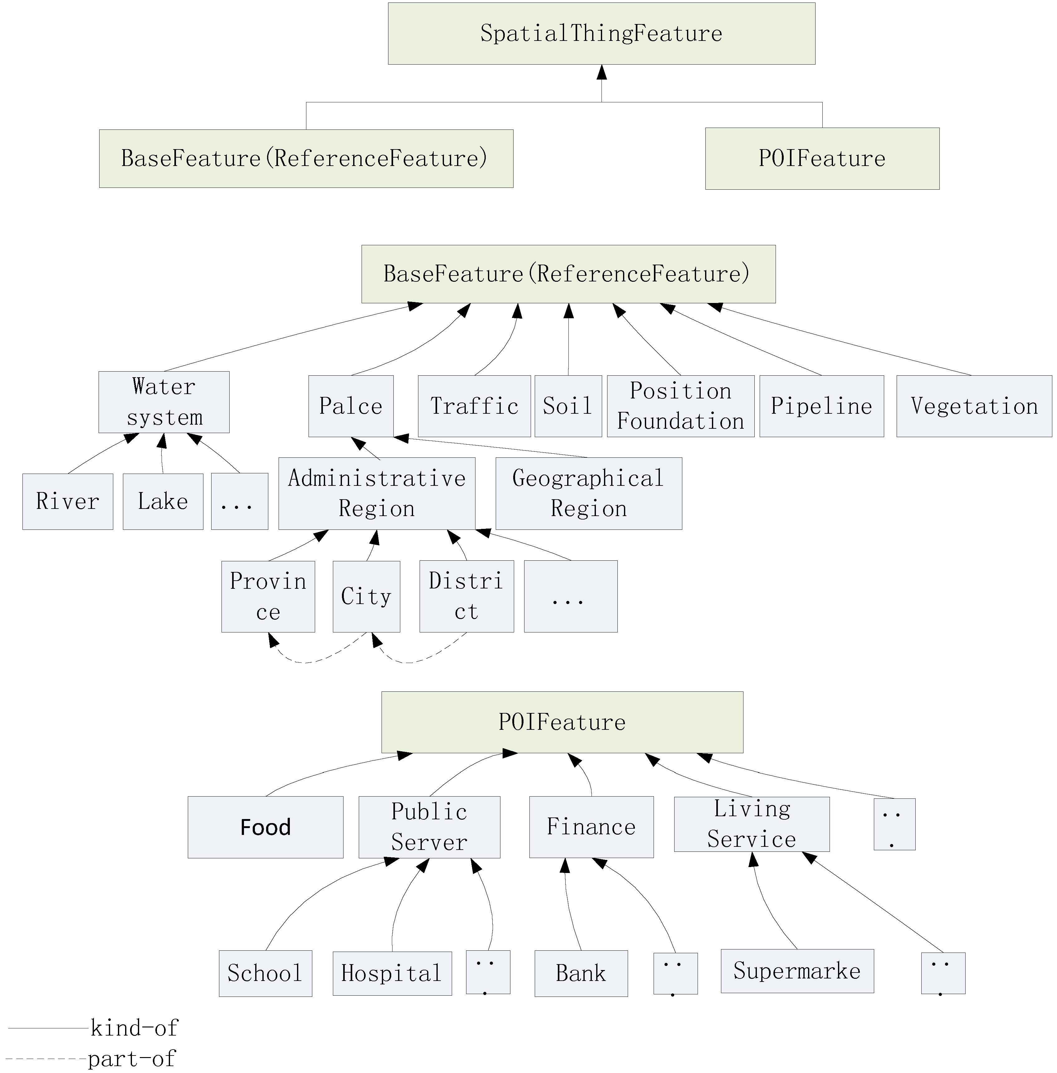
3.3. Ontological Classification of Geographic Features

The SpatialThingFeature class is the base component of DBSCANO. SpatialThingFeature can be hierarchically classified into BaseFeature (ReferenceFeature) and POIFeature. This means that SpatialThingFeature is a super-concept of BaseFeature and POIFeature. Certain relations (such as directions) are defined between a fixed reference object and a primary object (such as “a is to the left of the Thames”, “b is to the right of the Thames”). The primary and reference objects help define these DBSCAN relations. Together, the reference objects establish a reference frame that helps us determine the spatial relations of the primary object relative to the reference object. The reference objects are defined in reference to the “BaseFeature” set. For example, in the statement “ATM1 is to the left of the Thames”, ATM1 is the primary object and Thames is the reference object. The reference object is an instance of the “river” class, which is a sub-concept of BaseFeature. Because of this reference function, BaseFeature is also called ReferenceFeature. The class hierarchy can be illustrated as shown in Figure 7.

Let “district” be a kind of the “place name”. Relationships in DBSCANO exhibit certain correlations between geospatial and non-geospatial attributes of geographic elements (e.g., a bank may be inside a block, where “bank” and “block” are concepts and “inside” is a geospatial relation). Geographic individuals are instances of concepts in DBSCANO. In this paper, geographic individuals are typically important geographic objects, such as the Yangtze and Hanjiang Rivers. The DBSCAN ontology relationships are predominantly taxonomic and associative relationships. The structural classification of SpatialThingFeature is a hierarchical classification tree (e.g., a stream or ocean is a type of water system), and the spatial and non-spatial relations between the concepts in the tree (e.g., left_of, close_to, part_of, and kind_of) form the tree structure.

3.4. Ontological Classification of the DBSCAN Algorithm

The structure of the DBSCAN ontology is motivated by the need to provide essential knowledge about DBSCAN. This information is used to constrain the DBSCAN process and make the resulting clusters more meaningful. Within the DBSCANO framework, the DBSCANAlgorithm class provides a means of describing the functions offered by the algorithm. DBSCANAlgorithm describes a function of basic information types, namely, the function computed by the service.

An essential component of DBSCANO is the specification of DBSCAN. DBSCANAlgorithm represents two aspects of the functionality of the algorithm: the transformation of information (represented by inputs and outputs) and the state change (represented by parameter values) produced upon applying the constraints. To complete the clustering, we require both a geospatial dataset as input and the precondition that the ontology of the dataset actually exists. The clustering result is the output of the specified constraints and confirms the proper execution of the clustering transaction.

The major ontology classes represent the functions and parameters in the DBSCAN algorithm. These classes are further divided into sub-classes via “is-a” or “part-of” relationships. The class hierarchy thus developed can be illustrated as shown in Figure 8.

3.5. Ontological Classification of DBSCAN Relations

In a general ontology, the semantic relationships are most often expressed as “part-of”, “kind-of”, “attribute-of”, and ‘instance-of’ relations. In a geographic ontology, with the exception of general non-geospatial relationships, the most important relations are geographic geospatial relationships. The proposed geospatial relations contained in the geographic feature ontology introduced above are defined in terms of an ontology of 3-tuples of the form SR-Ontology = {<Space, Objects, Relations>} [12]. The Space set describes the geography of the domain, and the set of Objects contains the geospatial entities of interest and their associated attributes, which are defined in the geospatial feature ontology.

Geographic instances and DBSCAN’s specific function objects are instances of concepts combined with relationships and rules that express the DBSCAN domain knowledge. For example, a valid geographic instance would be represented as (University of Wuhan, Wuchang District). Rules and relationships are used to express the geographical background knowledge and to constrain the clustering of classes or instances (e.g., a particular district may be near the Yangtze River, and a particular POI may be defined as being to the left of a reference object, which must then constrain another POI that is to the right of the same reference object). The geographic feature ontology for clustering is expressed using a formal clustering representation language with unambiguous semantics.

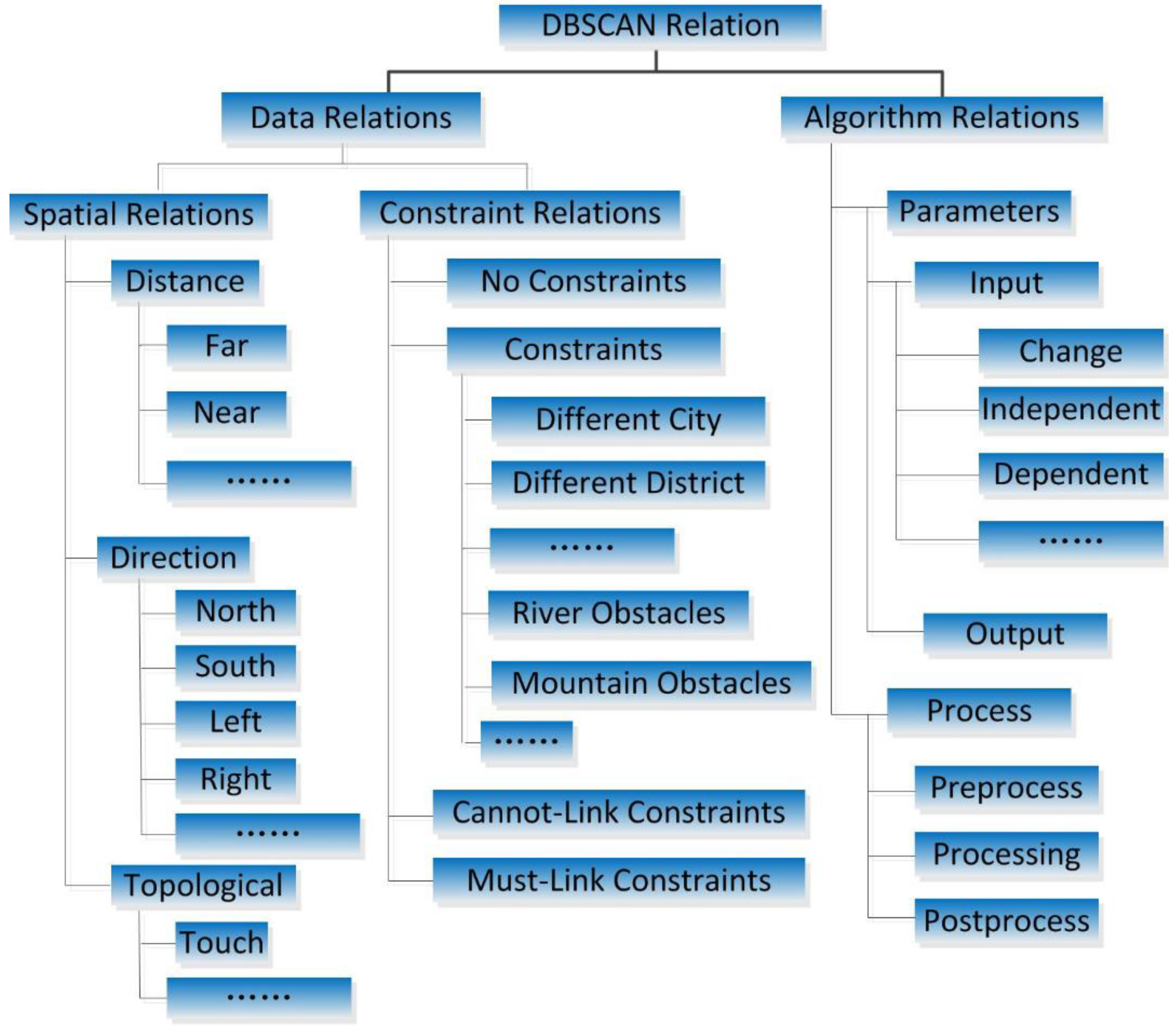
In DBSCANO, the “constraint relations” and “algorithm relations” play an important role in clustering. Constraint relations are transitive relations, whereas algorithm relations are asymmetric. The incorporation of such constraint and algorithm relations into clustering algorithms has not yet been well investigated. Our work in this paper will demonstrate that real geospatial problems require richer relations to express relevant domain knowledge.

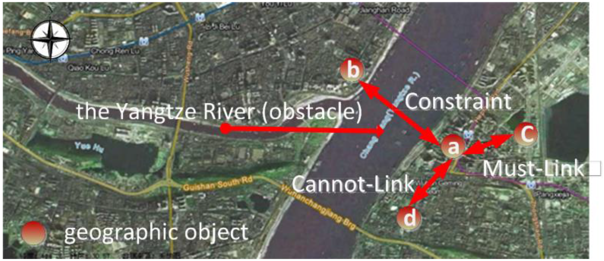
Constraint relations often require relational information that applies to a subset of geospatial objects. Constraint relations can be relations corresponding to "No Constraints”, “Constraints”, “Cannot-Link Constraints” or “Must-Link Constraints”. If two objects possess “No Constraints” relations with respect to an obstacle, then DBSCANO will allow the distance between them to be directly calculated. If two objects possess “Constraints” relations with respect to an obstacle, then DBSCANO will add some penalty to reflect these constraints, e.g., the time required to cross a river when traveling from one side to the other, when determining whether to place the objects in the same cluster. If two objects possess “Cannot-Link Constraints” in relation to each other, then DBSCANO will not allow them to be placed in the same cluster. If two objects possess “Must-Link Constraints” in relation to each other, then DBSCANO will ensure that they are placed in the same cluster.

Algorithm relations express relational information that applies to the DBSCAN algorithm. Such information primarily concerns the relationships between parameters in DBSCAN. The role of “Parameters” is to enable the flexible adjustment of Eps and MinPts in DBSCAN. Algorithm relations describe the relationships among the datasets in DBSCAN, Eps, and MinPts. Based on the context of the datasets being analyzed using DBSCAN, it is possible to infer appropriate values for Eps and MinPts. Background knowledge about these datasets can dramatically influence the values of Eps and MinPts. Another type of relation, “Process”, describes the ontology of the algorithm processes, which will be convenient for future expansion of the model.

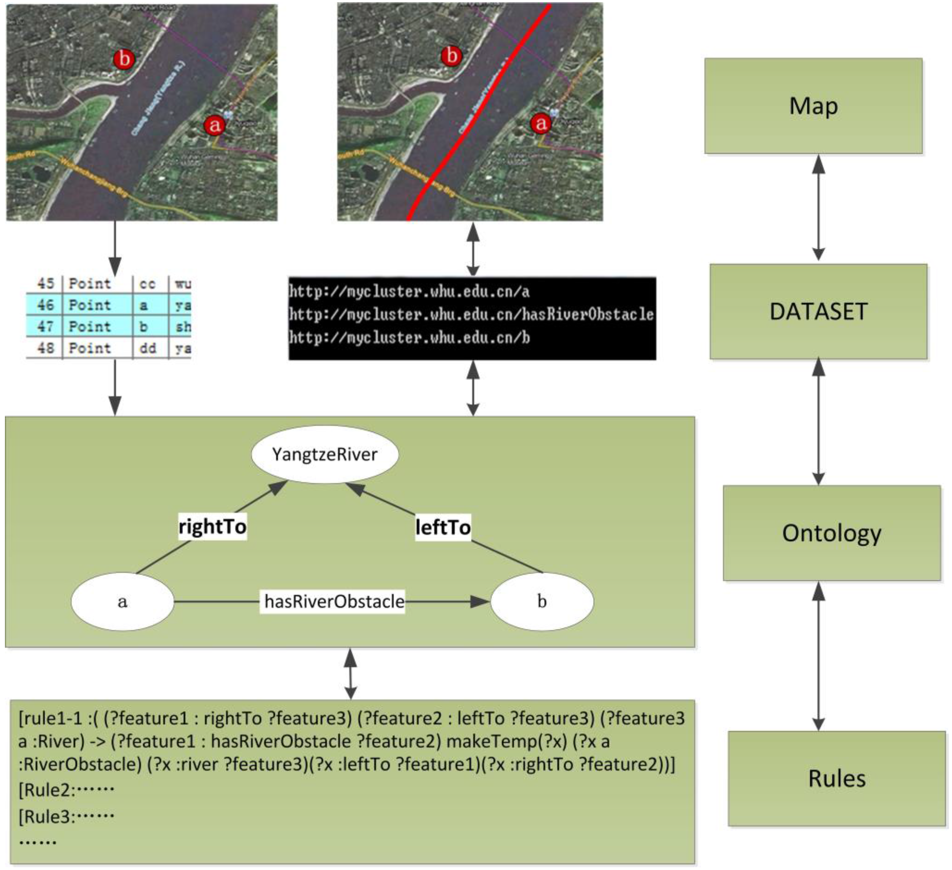
The structure of the geospatial relation ontology is illustrated in Figure 9. These relationships can be dynamically edited and expanded. An example of obstacle constraints between points a and b is illustrated in Figure 10.

Several properties and relations of objects exist in DBSCANO that can be used for reasoning, such as inverse, transitivity, and asymmetry properties and kind-of, part-of, instance-of, and attribute-of relations.

For example, an example of the transitivity property is as follows:

Let us say that there is an object transitivity property left_Of, indicated by the notation TransitivityProperty. That is, if a is to the left of b and b is to the left of c, then a is to the left of c.

Consider the following axioms:

• TransitivityProperty (leftOf)
• leftOf (a, b)
• leftOf (b, c)

Then, the assertion leftOf (a, c) is valid.

Let us say that leftOf is also an object asymmetry property, indicated by the notation AsymmetryProperty. That is, if a is to the left of b, then b is not to the left of a.

Consider the following axioms:

• AsymmetryProperty (leftOf)
• leftOf (a, b)

Then, the assertion leftOf (b, a) is invalid.

The priorities for the constraints relations exist in DBSCANO can be used for reasoning. This priority-setting mechanism for the constraints relations is priority(“Cannot-Link Constraints”) > priority(“Constraints”) > priority(“No Constraints”) > priority(“Must-Link Constraints”). The rule system produces may choose the constraints relations with the highest priority as the constraints relations to the same pair of features when there are some multilateral constraint relations.

4. Processing: Reasoning in DBSCANO

4.1. Reasoning in DBSCANO

In the framework of the DBSCAN ontology, a reasoner based on dotNetRDF [13] is used to infer knowledge represented in DBSCANO. dotNetRDF is a kind of API Library for working with RDF (N3) and SPARQL based on C#/.NET. dotNetRDF includes a powerful API for working with Apache Jena. The user constraints serve as the input to the reasoner, and the output is a set of meaningful geospatial clusters and datasets.

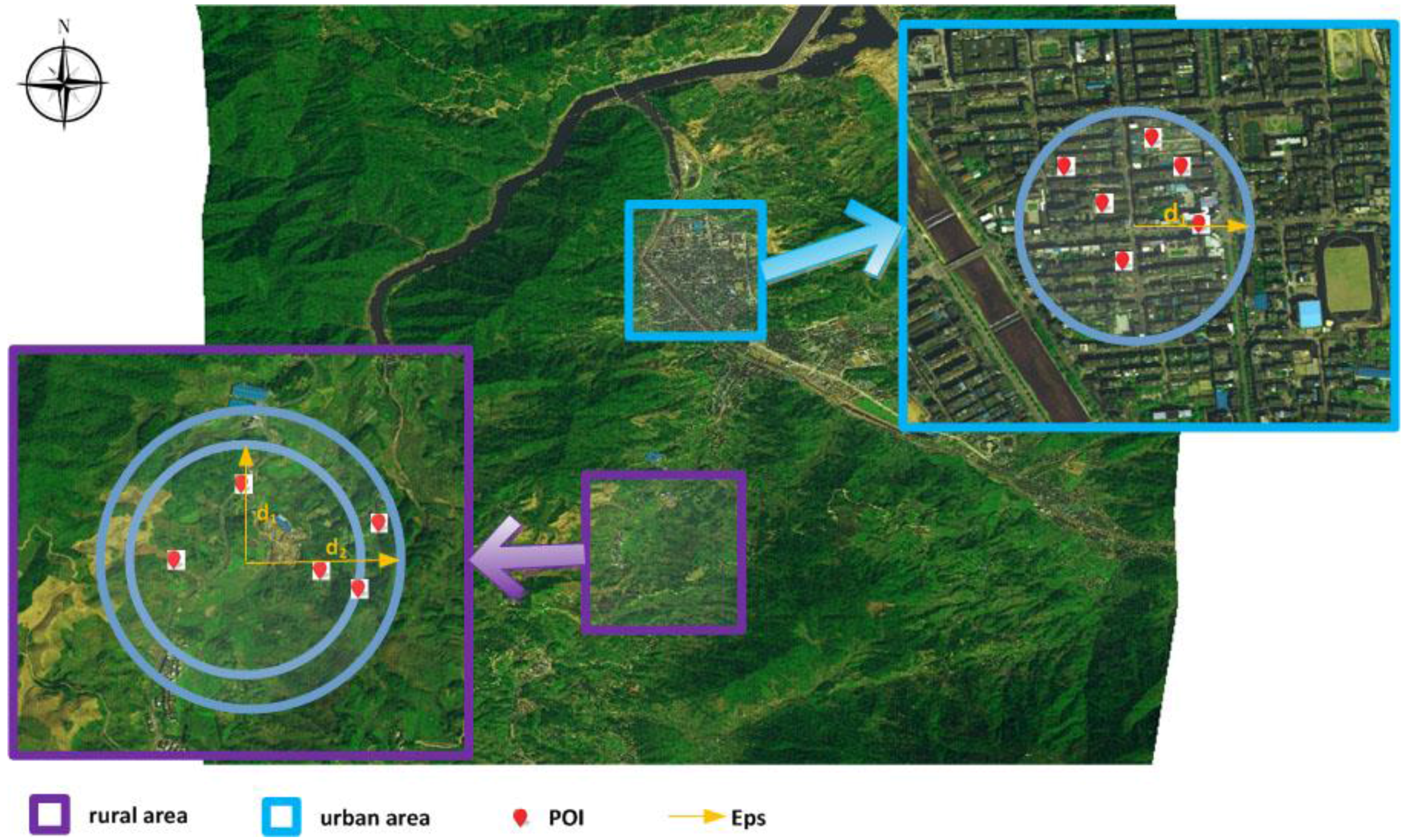
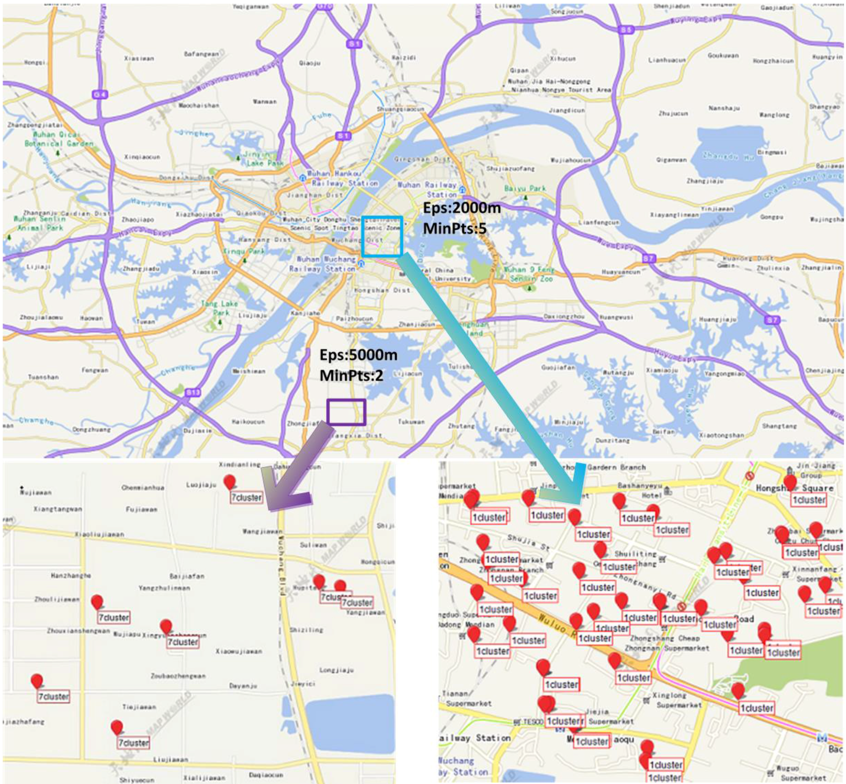
The DBSCANO reasoner first builds all SpatialThingFeature instances, thereby associating the reasoning with the geospatial clustering ontology and the user’s objective. For Example 1 presented in Section 3.1, the SpatialThingFeature instance “schools in Wuhan” is created using a Web Feature Service. The reasoner then builds an instance of DBSCANAlgorithm that contains several input instances. For example, the two instances “urban area parameter (Eps: 2000 m)” and “suburban area parameter (Eps: 5000 m)” are created by domain experts.

Next, the DBSCANO reasoner builds constraint rules using Jena rules. These Jena rules serve as a bridge between the geospatial datasets and the DBSCAN algorithm and are intended to assist in reasoning in combination with DBSCANO. The DBSCAN constraints are Jena rules that represent the dependencies between relationships and properties in DBSCANO. We use a rule-oriented model to share constraint-based knowledge in DBSCAN with experts. Rules built into DBSCAN provide the user with comprehensible and explicit constraints on the reasoning. DBSCAN can model the constraints described by a specific set of inputs and the strategy used to construct the geospatial dataset(s).

Finally, the reasoner inputs the resulting constraint knowledge into DBSCAN. These results can be translated into other inference models or languages.

4.2. Rules for Constraint Generation Based on DBSCANO

The generation of constraints in our ontology-aided DBSCANO algorithm proceeds as follows. Prior background knowledge is injected into the constraints on DBSCAN that are integrated into the density-based clustering task. These are obtained by means of the reasoning rules, which are typically generated by geospatial experts (e.g., using the GIS clustering literature). Thus, the manual analysis and mining of spatial data (such as for spatial association rules) proceeds semi-automatically. The task of producing the rules that constrain our knowledge is not discussed in detail here. In this paper, we assume that these geospatial constraint rules have been previously generated and that the constraint rules generated based on Jena rules determine the constraints that influence the clustering results obtained using the DBSCAN algorithm.

Definition 1: 

Let KB be the Description Logic (DL) knowledge of DBSCAN with constraints, including the geographic data constraints for clustering. We use the standard definitions for the constraint rules. A rule based on DBSCANO has the following form:

$$Rul{e}_{DBSCANO}::==Implies(Antecedent(A_{DBSCANO}),Consequent(B_{DBSCANO}))$$

where A_DBSCANO and B_DBSCANO are conjunctions of Jena rule atoms based on DBSCANO. The set of atoms B_DBSCANO is called the rule head, and the set of atoms A_DBSCANO is called the rule body. The atoms in A_DBSCANO can be of the form C(x), P(x, y), or builtIn(r, x ...), where C is an N3 description or data range of DBSCANO; P is a DBSCANO property; r is a built-in relation; and x and y are either variables, individuals, or data values. The atoms in B_DBSCANO may also refer to individuals, data literals, individual variables, or data variables; however, B_DBSCANO is limited to the form P(x, y), where P is the property of a constraint or parameter in DBSCANO and x and y are variables, individuals, or data values.

Based on problems that need to be solved above, we summarize that there are 2 types of reasoning rules used in this paper:

1. reasoning of constraints relationship by geographical background knowledge:

Definition 2: 

Rule_Constraints ::= Implies(Antecedent(A_{SpatialThingFeature}),Consequent(B_constraints))

A_{SpatialThingFeature} is a set of atoms based on SpatialThingFeature. B_constraints is an expression of the form: {atom_constraints} where at least on of {atom_constraints} is a constraint Property atoms.

2. reasoning of appropriate values of Eps and MinPts

Definition 3: 

Rule_Eps&MinPts ::= Implies(Antecedent(A_Eps&MinPts),Consequent(B_Eps&MinPts))

A_Eps&MinPts is a set of atoms based on SpatialThingFeature and DBSCANAlgorithm.B_Eps&MinPts is an expression of the form: {atom_Eps&MinPts} where {atom_Eps&MinPts}are “hasparameter” (“hasEps” or “hasMinPts”) Property atoms.

4.3. Knowledge Base of DBSCAN with Constraints

Let KB_DBSCANO be the knowledge base of DBSCAN with constraints. It has the following form:

$$K{B}_{DBSCANO}::==(\mathsf{\Sigma },\prod )$$

where ∑ is DBSCANO and ∏ is Rule_DBSCANO, which is a rule base for DBSCANO. A set of rules in ∑ can be used to infer new constraint knowledge from DBSCANO. The contents of the ontology in ∏ and the rules in ∑ can be dynamically expanded, modified, and deleted.

4.4. An Example of Reasoning

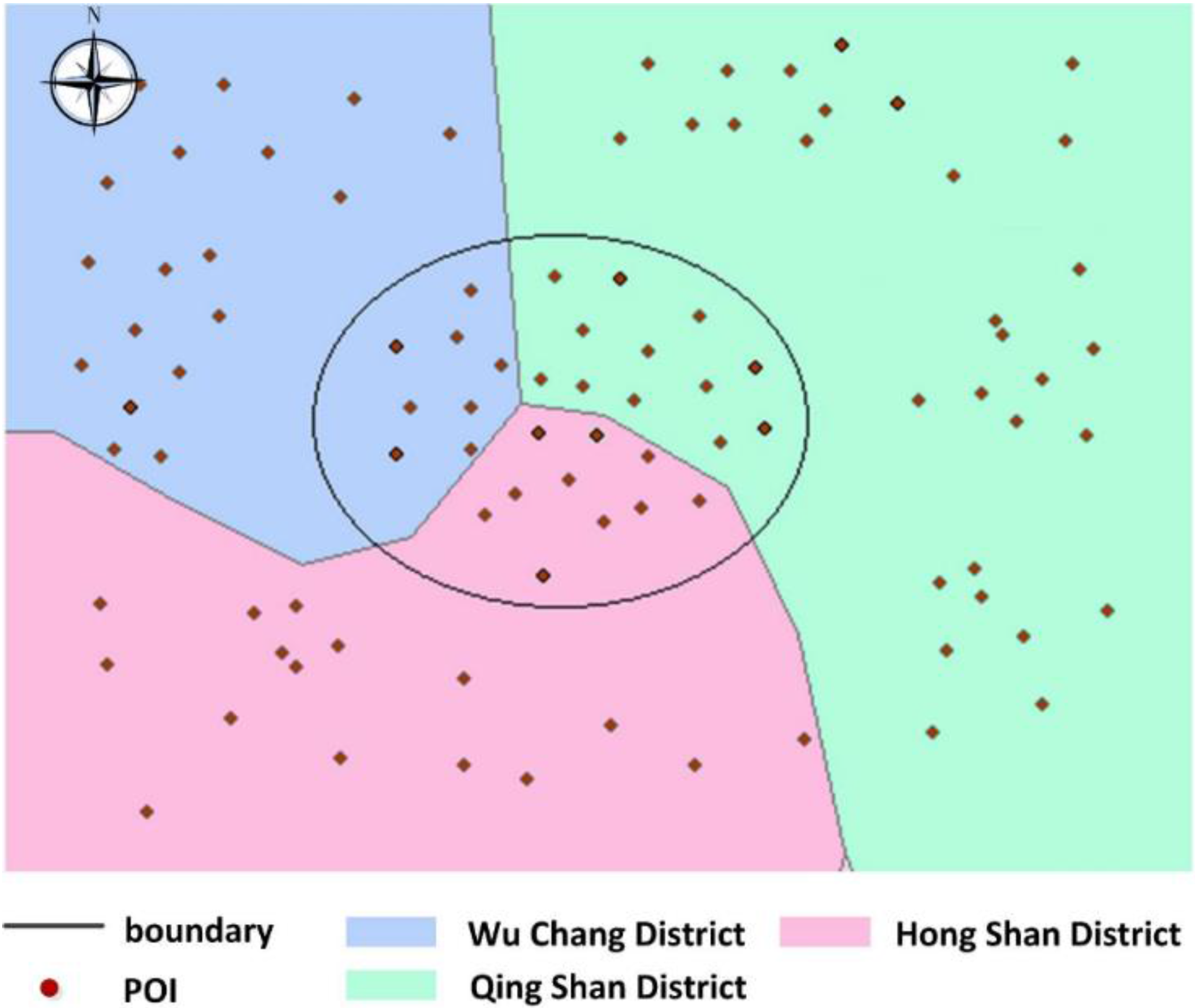
We define point a on the right side of the Yangtze River and point b on the left side (Figure 10 obstacle constraint). We define point a belonging to the wuchang district and point c belonging to the wuchang district (Figure 10 Must-Link). We define point d belonging to the hongshan district (Figure 10 Cannot-Link). By Jena rule reasoning, ab two points are regarded as a geospatial cluster with an obstacle constraint. a and c are regarded as a geospatial cluster with a Must-Link constraint. Similarly, a and d are regarded as a geospatial cluster with a Cannot-Link constraint. The following are the definitions of points a, b, c and d, the property “hasRiverObstacle”, “hasMustLink” and “hasCannotLink” and the relevant rules.

Algorithm 1. The Definitions of Points a, b, c and d, the Property “hasRiverObstacle”, “hasMustLink” and “hasCannotLink” and the Relevant Rules.

1: :a rdf:type:ATM,

2:       :POIFeature;

3:   :rightTo:YangtzeRiver;

4:    :hasBelongDistrict:wuchang.

5: :b rdf:type:ATM,

6:       : POIFeature;

7:   :leftTo:YangtzeRiver.

8: :c rdf:type:ATM,

9:       :POIFeature;

10:  hasBelongDistrict:wuchang.

11: :d rdf:type:ATM,

12:       :POIFeature;

13:  hasBelongDistrict:hongshan.

14: :YangtzeRiver a:River, :RiverObstacle;

15:   :name “YangtzeRiver”.

16: :leftTo rdf:type:Direction;

17:   owl:inverseOf:righTo.

18: :rightTo rdf:type:Direction;

19:   owl:inverseOf:leftTo.

20: hasRiverObstacle rdf:type:ObjectProperty;

21:  rdfs:domain:POIFeature;

22:  rdfs:range:POIFeature;

23:  rdfs:subPropertyOf:hasConstraint.

24: hasMustLink rdf:type :ObjectProperty;

25:   rdfs:domain:POIFeature;

26:   rdfs:range:POIFeature.

27: hasCannotLink rdf:type:ObjectProperty;

28:   rdfs:domain:POIFeature;

29:   rdfs:range:POIFeature.

[rule1-1 :( (?feature1 : rightTo ?feature3) (?feature2 : leftTo ?feature3) (?feature3 a :River) -> (?feature1 : hasRiverObstacle ?feature2) (?feature3 a :RiverObstacle) (?feature3 :name ?name))]

[rule1-2 :(?feature1 :hasBelongDistrict ?a) (?feature2 :hasBelongDistrict ?b) notEqual (?feature1,?feature2) Equal(?a,?b)-> (?feature1 :hasMustLink ?feature2)]

[rule1-3 :(?feature1 :hasBelongDistrict ?a) (?feature2 :hasBelongDistrict ?b) notEqual (?feature1,?feature2) notEqual(?a,?b)-> (?feature1 :hasCannotLink ?feature2)]

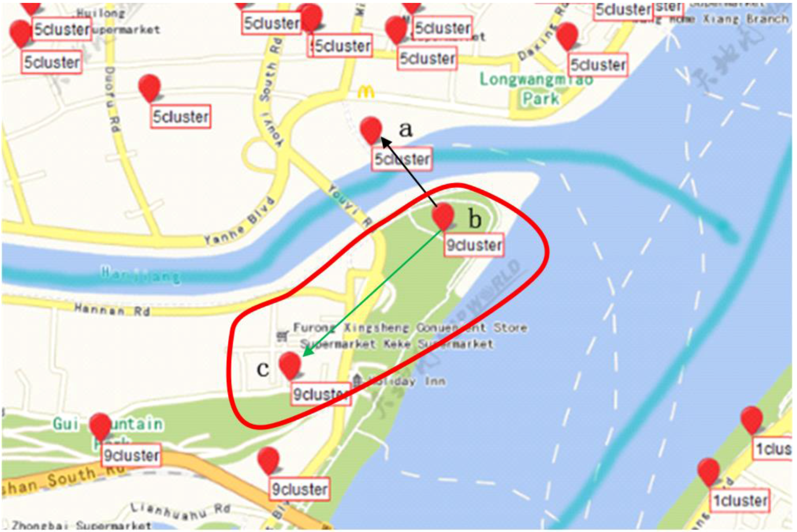
According to above rule1-1, constraints can be obtained by reasoning under this algorithm shown in Figure 11.

The definitions of point e and appropriate values for Eps and MinPts in Figure 2 are given below.

Algorithm 2. Definitions of Point e and Appropriate Values for Eps and MinPts.

1: :e rdf:type :ATM,

2:      : POIFeature;

3:  :location : hedong.

4: : hedong rdf:type :placeName,

5:       : suburb1.

6: : suburb1 rdf:type : districtType;

7:      : hasEps : EpsA;

8:     : hasMinPts : MinPtsA.

9: : EpsA rdf:type : Eps;

10:     :hasValue 5000.

11: : MinPtsA rdf:type : MinPts;

12:     :hasValue 3.

[rule2 :(?p : location :?a) (?a : type ?b) (?b : hasEps ?c)-> (?p : hasEps ?c) (?p : hasMinPts ?c)]

4.5. Improving the Distance Function in the Presence of Obstacles

Improving the distance function is one of the most important steps of DBSCAN. In this paper, we redefine the obstacle distance in the DBSCAN algorithm using ontology-aided constraints. The new distance function is dist’(p, q), which denotes the shortest distance from object p to object q considering any obstacles. The portion of the path that is cut off by any obstructions between the two objects is called the obstacle distance. We define

$$\mathrm{dist}\prime \left(p,q\right)=\{\begin{array}{c}dist(p,q),\text{ p not hasConstraint q}\\ dist\left(\mathrm{p},v_{\min Start}\right)+dist\left(v_{\min Start},v_{\min End}\right)+dist\left(v_{\min end},\mathrm{q}\right),\text{p hasConstraint q and p can be linked with q}\\ \infty ,\text{p hasConstraint q and p must not be linked with q}\\ 0,\text{p hasConstraint q and p must be linked with q}\end{array}$$

(1)

where dist(a, b) is the distance function that computes the shortest path between points a and b using the Mahalanobis distance, the Euclidean distance, or some other distance measure. Let Vertex(obstacle) = {v_1, v_2,..., v_n} be the set of all border points on the obstacle, and consider the path around the border of the obstacle.

The function dist’(p, q) is used in the proposed algorithm. This function expresses geographic semantic meaning as follows:

(1)

Certain geographic objects are not regarded as obstacles in the clustering analysis, such as air routes or overhead high-voltage lines between POIs.

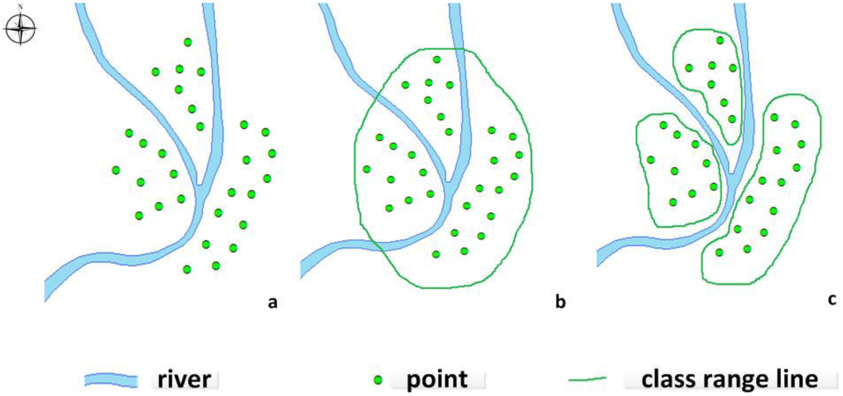
(2)

Certain geographic objects represent barriers that cannot be ignored, such as a river between two points connected by bridges.

(3)

Certain geographic objects must be prohibited from being clustered because of class constraints, such as two points in different administrative regions when the task is to cluster objects within administrative regions.

(4)

However, certain geographic objects must be assigned to the same cluster because of certain class constraints even in the case of conflicting constraints, such as two points in different administrative regions that belong to the same company when the first priority in the clustering task in placed on the company affiliation.

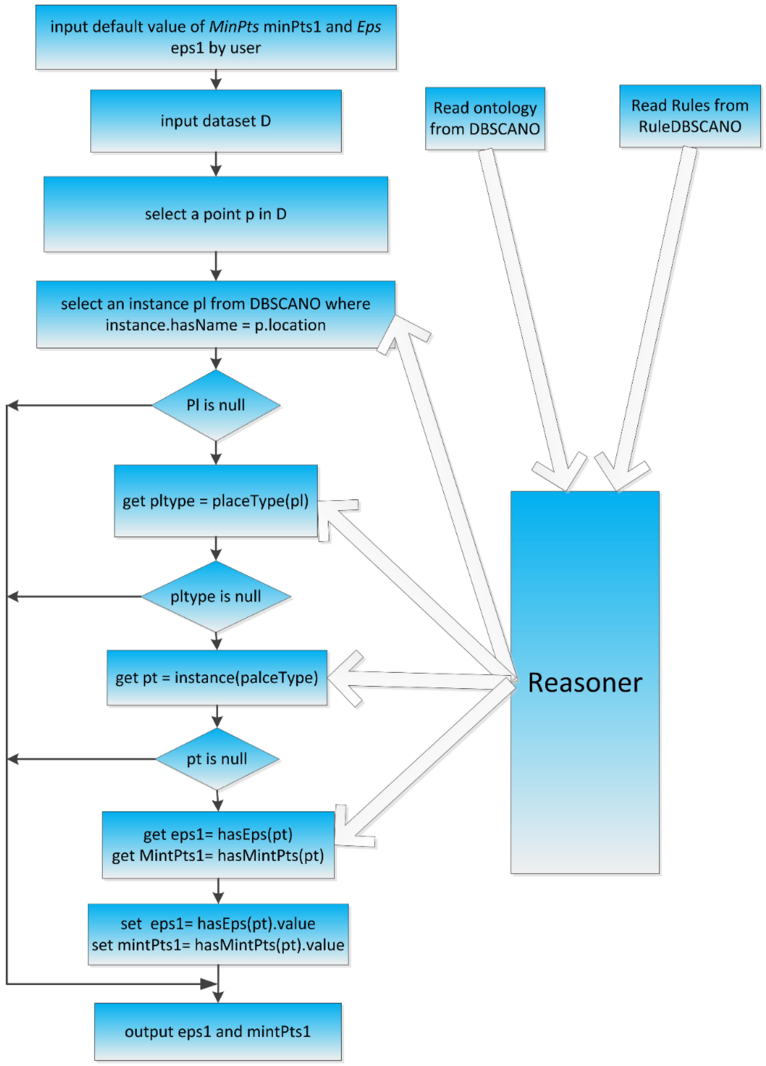
4.6. Determining Appropriate Values for Eps and MinPts

Determining appropriate values for Eps and MinPts is another important task. In this step of the process, the algorithm uses reasoning to obtain appropriate values based on the dataset to be clustered. The DBSCAN algorithm with constraints acquires values for Eps and MinPts as follows:

(1)

The user sets certain default values of Eps and MinPts. The program reads the ontology from DBSCANO and the rules from Rule_DBSCANO.

(2)

While the program is running, ontological reasoning yields appropriate values of Eps and MinPts for the dataset to be clustered. This dataset is used to determine the values of Eps and MinPts. The reasoning performed for this purpose is currently based on dotNetRDF, which supports both static and dynamic reasoners, i.e., those that use a fixed set of rules for Eps and MinPts and those that create their rules dynamically based on the input spatial data.

(3)

If the process does not generate appropriate values of Eps and MinPts automatically, then these parameters return to their default values.

The overall flow of the reasoning process for determining Eps and MinPts is illustrated in Figure 12.

4.7. Inference Engine

The ontology-aided DBSCAN algorithm with constraints involves several additional functions compared with the standard DBSCAN algorithm, which represent calls to the reasoning engine. Depending on the properties of the problem context (data inputs), various functional units are invoked to solve a clustering problem with constraints.

We adapted the DBSCAN algorithm in accordance with the ontology system discussed above. The adapted algorithm is similar to the original, with the addition of semantic constraints. The main additional functions are described in Algorithm 3. The infer ence engine in Algorithm 1 is used to compute the constraint relationships between instances in the ontology “SpatialThingFeature” and to obtain multiple parameters for application in the clustering process.

Algorithm 3. DBSCAN algorithm with ontology-based background knowledge.

1: DBSCANWithOntology (InputData, Eps, MinPts)

2:  D = InputData

3:  cluster = null

4: clusterID = 0

5:  for each point P of D

6:  set P.status as unvisited

7:  for i = 0 to D.count—1

8:  P = D.get(i)

9: if (P.status is unvisited)

10: newEps = testParameterOf Eps(p)

11: if (newEps != Eps)

12: Eps = newEps

13: MinPts = testParameterOf MinPts (MinPts)

14: set P.status as visited

15:  NeighborPoints = searchNeighborPoints(P, Eps)

16:  if (NeighborPoints.length < MinPts)

17:    label P as NOISE

18:  else

19:    add P to cluster[clusterID++]

20:  for each point P’ in NeighborPoints

21:    if (P’.status is visited)

22:     mark P’.status as visited

23:     NeighborPoints’ = searchNeighborPoints(P’, Eps)

24:     if (NeighborPoints’.length >= MinPts)

25:      NeighborPoints = NeighborPoints combined with NeighborPoints’

26:    if (P’ does not belong to any cluster)

27:     add P’ to cluster[clusterID]

28:  return cluster

29: searchNeighborPoints(P, Eps)

30:  pAll = all points within the Eps neighborhood of P (including P)

31:  PNewSet = null

32: for each point P’ in pAll

33:  if (dist’(P, P’) <= Eps)

34:    add P’ to cluster PNewSet

35: return PNewSet

36: dist’(p, q)

37: distance = 0

38: constraint = testIsConstraint(p, q)

39: if (constraint ==null|| constraint = noHasConstraint)

40:    distance = dist(p, q)

41: if (constraint ==hasConstraint)

42:  vmidStart = getMidStart(p,q)

43:  vmidEnd = getMidEnd(p,q)

44: distance = dist(p, vmidStart) + dist(vmidStart, vmidEnd) + dist(vmidEnd, q)

45: if (constraint ==hasCannotLink)

46: distance = Eps + constant(>0)

47: if (constraint ==hasMustLink)

48: distance = 0

49: return distance

50: testParameterOf Eps(p)

51: return Eps via reasoning based on p

52: testParameterOf MinPts(p)

53: return MinPts via reasoning based on p

54: testIsConstraint(p1, p2)

55:  return type for the presence of a constraint relation between p1 and p2

The DBSCAN algorithm ontology structure view is shown in Figure 13.

DBSCAN requires approximately O (N²) time, where N is the number of points in the datasets. For the analysis of an additional constraint operation function with geographical background constraints using a semantic expression in DBSCANWithOntology, the time complexity for {testParameterOfEps, testParameterOfMinPts, testIsConstraint} is at most the square of the number of points n.

5. Experimental Concrete Implementation: A Software Prototype

5.1. Prototype of the Ontology-Aided DBSCAN Algorithm with Constraints

We now demonstrate a prototype implementation of DBSCAN with constraints based on an ontology (referred to as the C-DBSCANO algorithm). We used C# based on dotNetRDF to develop this prototype, and the ontology dataset was stored in SQLite. dotNetRDF is a powerful and flexible API for working with RDF and SPARQL in .NET environments. A data clustering task involves the following steps:

(1)

Ontology and rules are derived and extracted from relevant experts, data mining and knowledge discovery. The ontology and rules are obtained and stored in the database.

(2)

The user establishes a clustering model in the user interface.

(3)

The ontology and the rules stored in the dataset are selected from the data file in accordance with the settings of the clustering model.

(4)

Through reasoning over the rules, the constraint rules are obtained and fed into the DBSCAN module.

(5)

DBSCAN is run based on the algorithm knowledge.

(6)

The results of geospatial clustering with obstacle constraints are displayed on a web-based map.

The DBSCAN process was performed using dotNetRDF. Figure 14 shows the corresponding flow diagram. This process requires that thresholds be set for the Eps and MinPts parameters.

5.2. Evaluation Method

We examined the impact of constraints on the clustering results by applying C-DBSCANO, C-DBSCAN [14], and the original DBSCAN algorithm to real datasets acquired from online spatial data resources. Because the test dataset did not include constraints, we artificially inserted obstacle constraints, including real geographic data constraints consistent with the actual geography of the location corresponding to the dataset. The values of Eps and MinPts were set in the C-DBSCANO algorithm to be suitable for the test area of Wuhan city and its suburbs.

The first evaluation metric, used to evaluate and compare the accuracy of the three clustering algorithms, is the pairwise F-measure (PWF1) [15], which is the harmonic mean of the precision and recall for sample pairs:

$$\mathrm{PWF1}=\frac{2\times \mathrm{precision}\times \mathrm{recall}}{\mathrm{precision}+\mathrm{recall}}$$

where

$$\mathrm{precision}=\frac{\text{the number of pairs correctly placed in the same cluster}}{\text{the total number of pairs placed in the same cluster}}$$

$$\mathrm{recall}=\frac{\text{the number of pairs correctly placed in the same cluster}}{\text{the total number of pairs actually in the same cluster}}$$

The second metric is an efficiency measure to compare the run time of C-DBSCANO with those of the C-DBSCAN and DBSCAN algorithms.

All experiments were performed on a PC with a 2.1 GHz Intel CPU and 2 G of main memory running the 64-bit Windows 7 operating system.

6. Experimental Results and Discussion

6.1. Experimental Area

Wuhan (29°58′N to 31°22′N, 113°41′E to 115°05′E) is located in the eastern region of the Jianghan Plain. Wuhan comprises the three towns of Wuchang, Hankou, and Hanyang and is the capital of Hubei Province in central China. Wuhan lies at the intersection of the Yangtze River and the Hanjiang River. The three towns, which are separated by the waterways, are connected by many tunnels and bridges. For this paper, we selected Wuhan as the study area to empirically illustrate the application of DBSCAN with constraints using a semantic expression model of the geographical background.

The research area is large, and the administrative region is much more so; therefore, it is suitable for the testing of multi-region parameters for DBSCAN. Moreover, the area is full of rivers and lakes and thus is very suitable for the testing of clustering analyses with geographical barrier constraints.

6.2. Experiment: Primary School Data from Wuhan, China

In this section, we present the results obtained using our implementation of the C-DBSCANO algorithm.

For an application addressing primary schools, we performed a geospatial clustering analysis relevant to river obstacles and attribute constraints in Wuhan in central China. The available dataset consisted of 760 primary school records. The reasoning process applied in this application was similar to that described in Section 4.1.

The search city was “Wuhan”, the feature on which to perform the clustering analysis was set to “primary school”, MinPts was set to 5, and Eps was set to 2000 m.

The test results are shown in Figure 15 and Figure 16. From the results presented in Figure 15, we see that the obstacle constraints posed by the Hanjiang River caused point b to be clustered with point c rather than point a, despite the fact that the distance between a and b is less than the distance from c to b.

Figure 16 shows that, guided by ontological reasoning, the clustering parameters were automatically modified during execution. Thus, the urban-area parameters (Eps: 2000 m, MinPts: 3) were transformed into parameters suitable for suburban regions (Eps: 5000 m, MinPts: 2), following the rules established in the program’s knowledge base, which state that more densely populated urban areas will have a denser concentration of schools.

6.3. Evaluation over Instances

Table 1. Datasets used in the test.

Dataset	Name	Source of data	Number of Points
Dataset 1	banks	[16]	63
Dataset 2	supermarkets + hospitals	[16]	144
Dataset 3	primary schools	[17]	760
Dataset 4	hospitals	[17]	929

describes four datasets that were acquired from www.bing.com/maps and map.baidu.com (Dataset 1, Dataset 2, Dataset 3 and Dataset 4) and used as the basis of a performance comparison to more accurately evaluate the efficacy of the algorithm. The algorithms employed in this performance comparison were as follows:

• DBSCAN
• C-DBSCAN (randomly selected 5% of pairwise constraints)
• C-DBSCANO

6.4. Discussion

The results presented in Figure 17 and Figure 18 exhibit similar trends with respect to PWF1 and run time.

(1)

These results show that the proposed framework is capable of exploiting pairwise constraints to achieve improved clustering accuracy compared with DBSCAN and C-DBSCAN. As shown in Figure 17, the use of constraint knowledge by C-DBSCANO allows this algorithm to be more accurate than DBSCAN, which is very inaccurate compared with the other algorithms. Because C-DBSCAN includes no qualitative spatial constraints, its results are little better than those of DBSCAN.

(2)

As shown in Figure 18, C-DBSCANO does not outperform DBSCAN when the number of constraints is small. This is because the computation of the constraints requires additional time. C-DBSCANO is also less efficient than C-DBSCAN because some of the C-DBSCANO constraints are based on logical reasoning rather than numerical calculations. The speed of the reasoner based on dotNetRDF is slow; this is the primary shortcoming of C-DBSCANO and needs to be improved in future.

7. Conclusions

The purpose of adding geographical knowledge to DBSCAN using ontological expressions is to allow users to obtain representative and useful clustering results. Using the approach proposed in this paper, C-DBSCANO improves the rationality of clustering in three important aspects. First, it considers the clustering constraints imposed by the real geographical environment, using an ontology-based semantic modeling approach to regulate these constraints in geographical space. Second, this method avoids unreasonable or inflexible clustering processes and also guides the DBSCAN program through reasoning based on a geospatial clustering ontology to adjust the clustering parameters. This DBSCAN algorithm ontology allows the clustering function to be extended and generalized. The DBSCAN algorithm ontology provides a particular class of functionalities while adhering to certain context-specific constraints. For example, the function may find appropriate parameters in accordance with the scale of the data. Third, the ontological model can be shared and exploited to allow more precise clustering knowledge to be discovered, thereby reducing the use of system resources. Although the data and the constraint knowledge are separated in the C-DBSCANO algorithm, the clustering analysis of the constraints is expressed in the ontological knowledge base. This enables the constraint knowledge to be dynamically edited to appropriately guide clustering analyses in different scenarios.

The proposed method combines both spatial and non-spatial constraint attributes. The implemented demonstration of the method proved that the method proposed in this paper, which incorporates geographical background constraints using a semantic expression model, is effective. However, the use of geo-ontologies in the C-DBSCANO algorithm as considered in this paper focused only on practical clustering applications. The use of more complex geographical background constraints will be an important direction of research in the future. We intend to expand our geospatial clustering ontologies to allow them to express a greater abundance of semantic geospatial relationships. The current spatial clustering algorithm is most effective in confined areas, but we will study effective multi-scale clustering with the aim of achieving multi-scale spatial clustering with constraints.