Hidden Naive Bayes Indoor Fingerprinting Localization Based on Best-Discriminating AP Selection

Abstract

Indoor fingerprinting localization approaches estimate the location of a mobile object by matching observations of received signal strengths (RSS) from access points (APs) with fingerprint records. In real WLAN environments, there are more and more APs available, with interference between them, which increases the localization difficulty and computational consumption. To cope with this, a novel AP selection method, LocalReliefF-C( a novel method based on ReliefF and correlation coefficient), is proposed. Firstly, on each reference location, the positioning capability of APs is ranked by calculating classification weights. Then, redundant APs are removed via computing the correlations between APs. Finally, the set of best-discriminating APs of each reference location is obtained, which will be used as the input features when the location is estimated. Furthermore, an effective clustering method is adopted to group locations into clusters according to the common subsets of the best-discriminating APs of these locations. In the online stage, firstly, the sequence of RSS observations is collected to calculate the set of the best-discriminating APs on the given location, which is subsequently used to compare with cluster keys in order to determine the target cluster. Then, hidden naive Bayes (HNB) is introduced to estimate the target location, which depicts the real WLAN environment more accurately and takes into account the mutual interaction of the APs. The experiments are conducted in the School of Environmental Science and Spatial Informatics at the China University of Mining and Technology. The results validate the effectiveness of the proposed methods on improving localization accuracy and reducing the computational consumption.

1. Introduction

Currently, with the popularity of smart phones and the development of mobile Internet, a great deal of location-based services (LBS) emerges, such as e-advertisements for customers walking in shopping malls and for cars locating services in underground parking lots. The user location sensing unit, the fundamental component of LBS, has played a key role in the whole application. There is an urgent need for an approach that can accurately collects moving users’ position in a short time. As a mature technology, GPS has been widely used in outdoor positioning, but it cannot be used in indoor positioning since the signal is blocked by the building [1,2,3,4]. At present, due to the complexity of indoor localization, there is not yet a widely-recognized strategy that is suitable for all kinds of unique indoor environments. Therefore, indoor localization has become a research focus and has attracted more and more attention from researchers.

Many indoor positioning methods have been proposed, which can be divided into two categories according to their measurement and positioning principles. The first category is geometric methods, including the trilateration and triangulation. Methods of trilateration estimate the position of a mobile object by measuring its distance between multiple reference locations. The distance is usually calculated using the signal attenuation model or the product of light speed and propagation time based on the prior measurement of time of arrival (TOA) or time difference of arrival (TDOA). As a typical method of trilateration, the ultra-wideband (UWB) technology of indoor positioning has become very popular recently. Methods using TOA need accurate time synchronization between the transmitter and the receiver. The triangulation technique, also named as the angle of arrival (AOA), makes use of the mobile object’s observing angles for two known positions to estimate the target position. There are two advantages of AOA technology: it does not need time synchronization and requires fewer observations. However, AOA also has two disadvantages. It requires additional hardware, such as an antenna array, which is expensive. Moreover, the positioning accuracy declines as the mobile object gets further away [5,6,7].

Fingerprinting localization, the second category of indoor positioning methods, is recognized as a main research direction owing to the following advantages: it is flexible and easy to realize; there is no need to know exactly the physical location of the APs; and it does not rely on additional hardware. The method consists of two stages: offline and online stages. During the offline stage, the fingerprint database is built up by means of site calibration. Firstly, in the region of interest, a number of reference location points is deployed according to a certain space. Secondly, for each reference location, the received signal strengths (RSS) from all of the APs in the region are collected. Finally, the fingerprint, a record consisting of the RSS vector and its corresponding location coordinates, is stored to establish a fingerprint database. During the online stage, the location estimation method compares the real-time observed RSS vector with the fingerprint database records and, afterwards, selects the position of the best-matched fingerprint record as the estimated result. According to fingerprint data types, fingerprinting algorithms can be divided into deterministic and probabilistic algorithms [8,9,10,11]. The deterministic algorithm stores the RSS value from each AP in the fingerprint database, whereas the probabilistic algorithm stores the RSS probability distribution model. The probabilistic algorithms are generally believed to be more effective because of their capability of dealing with the time variation of RSS [12,13,14].

With the widespread use of wireless LAN, there are more and more APs detectable in the environment. However, some of these APs are not helpful for positioning. Meanwhile, some APs are redundant as positioning references. Therefore, it is urgently needed to find a good strategy of finding the set of the most useful APs while effectively exploiting the interaction between APs. We have proposed a novel AP selection method, LocalReliefF-C (a novel method based on ReliefF and correlation coefficient), which can obtain the set of the best-discriminating APs for each reference location via removing useless and redundant APs. The process of AP selection reduces the dimension of the input vector used for positioning and, hence, brings lower computational complexity. In order to improve the positioning speed, we adopt an effective clustering method to divide the reference locations into several clusters. During the location estimation process, we firstly determine the target cluster through comparing the key of each cluster with the set of best-discriminating APs of the RSS observation sequence in this location and then import the hidden naive Bayes model to complete the task of inner-cluster positioning.

The main contributions of this paper are as follows:

• A novel AP selection method LocalReliefF-C has been put forward to obtain the set of best-discriminating APs for each reference location, which can reduce the positioning computational overhead and, meanwhile, achieve comparable positioning performance with the strategy using the full set of APs. The sets of the best-discriminating APs is then utilized by the effective clustering method of the fingerprint data.
• A fast and effective clustering method of fingerprint data has been proposed to narrow the search space and improve positioning performance, which puts the fingerprint records having the common subset of best-discriminating APs in one cluster. It is more efficient and easier to implement.
• The hidden naive Bayes model is applied to location estimation, which loosens the assumption of AP conditional independence and effectively utilizes the dependence of APs.

The rest of this paper is organized as follows: Section 2 introduces related work on AP selection and depicts the proposed AP selection method, LocalReliefF-C, in detail; Section 3 shows the fast clustering process of fingerprint records based on the sets of best-discriminating APs; Section 4 describes the location estimation method based on the hidden naive Bayes model; Section 5 gives the experimental design and results analysis; and Section 6 concludes the paper and gives suggestions for future research.

2. Access Points’ Selection Using LocalReliefF-C

2.1. Related Work on AP Selection

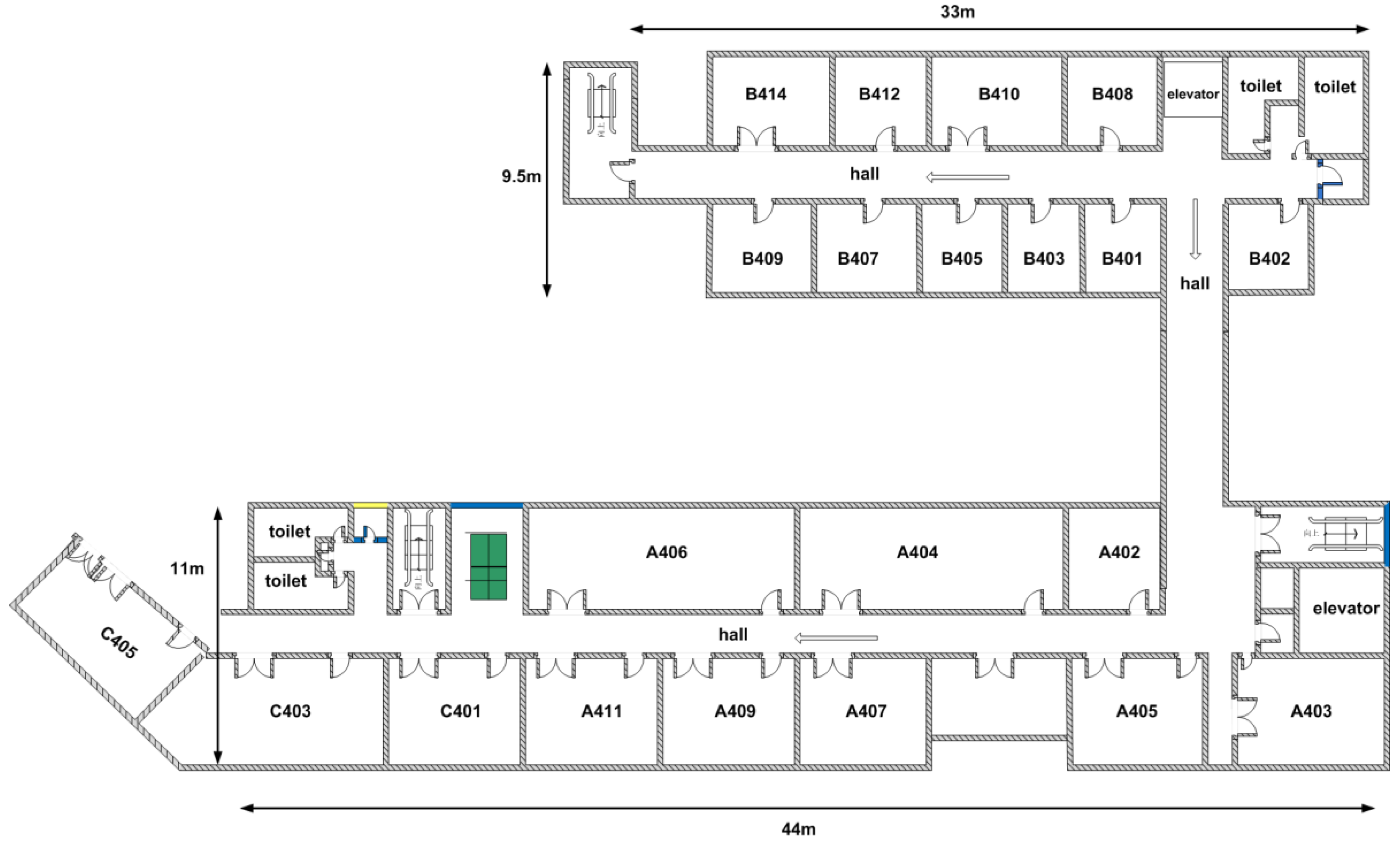
Pervasive wireless LAN facilities make WLAN indoor positioning technology feasible. However, sometimes, too many APs also increase the computational complexity and positioning difficulty. The number of detectable APs can often be up to 20 in all kinds of indoor environments, such as shopping malls, campuses, offices or homes. As an example,

Table 1. Number of detectable APs in China University of Mining and Technology (CUMT).

Location	Working Hours	Non-Working Hours
Administration Building	23	19
A College Office	13	11
Library Hall	15	15
Public Classroom	14	11
Students Dining hall	9	9

shows the average number of detectable APs of at a certain location in different indoor environments of the China University of Mining and Technology (CUMT) campus during working and non-working hours, respectively. Moreover, owing to the severe multipath effect of indoor signal propagation, the detectable AP set varies with the observation time and position. It has been pointed out that not all of the detectable APs can be utilized for positioning [15]. There are such APs that either act as a noise factor or play a redundant role in positioning. This inspires researchers to focus on the AP selection strategy for screening out the subset of APs that are necessary and sufficient for positioning and discarding the noisy and redundant ones.

Youssef et al. [16,17,18] have proposed the MaxMean method, which selects the first k strongest APs. In fact, they intuitively believe that the APs appearing most frequently in samples are needed. According to their analysis, the APs with the highest average signal strength are those that appear most frequently. This method is simple and effective; however, it may not be that complete in some circumstances. Specifically, since the wireless LAN hardware in a real environment is usually provided by several different manufactures, the average levels of signal strength received from them can be quite different. The MaxMean method is apt at discarding these APs with low average signal strength, which may appear frequently and contribute to positioning. Chen et al. [19] have provided the InfoGain method based on the information theory measure. The information gain, regarded as a measure of discriminative capabilities, is calculated for each AP and then ranked in a descending order. The first k APs corresponding to the highest information gain are finally selected. Lin et al. [20] have provided a group-discrimination-based AP selection method, which exploits the risk function from support vector machines (SVMs) to estimate the positioning capabilities for the AP group.

2.2. Proposed LocalReliefF-C AP Selection Method

Fusing the well-accepted feature selection algorithm ReliefF with the measure of the Pearson correlation coefficient, we have put forward a novel AP selection method called LocalReliefF-C, which can effectively estimate the positioning capability for each AP and determine the significant correlation between every two APs, which are potentially redundant. It can improve the positioning accuracy and reduce the computational overhead for positioning systems by means of discarding redundant APs and obtaining the set of the best-discriminating APs.

Up to now, several machine learning models have been applied to indoor positioning, such as naive Bayes, SVM, decision tree induction and neural networks [20,21]. Fingerprinting indoor positioning can be viewed as a multi-class classification problem in the machine learning field. The records of the fingerprint database correspond to training instances, while reference locations correspond to class labels. In a machine learning way, location estimation is actually to determine the class for the given new instance. Feature selection in machine leaning is the process of selecting a subset containing relevant features to use in model construction [22]. There are both similarities and differences between AP selection and feature selection. Even so, we still believe that with each AP viewed as a feature, it makes sense to introduce a classic feature selection method into AP selection for positioning.

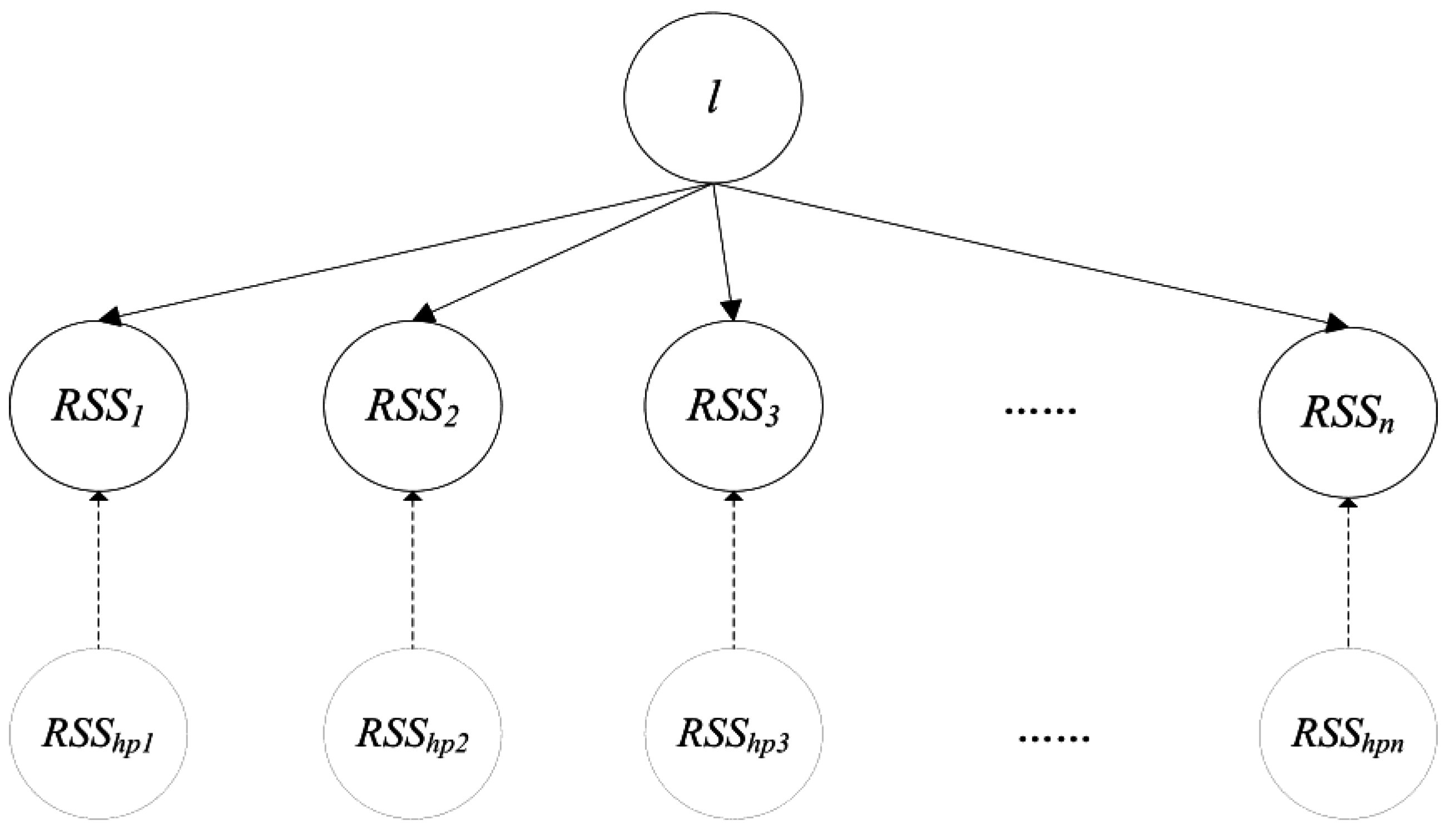
Relief is a well-accepted feature selection method for the two-class classification problem. It has the advantage of being simple to implement and having high running efficiency [23,24]. Its core idea is to select the subset of features with the best discriminating capability. The discriminating capability of each feature is represented by a weight, which is calculated according to how well the values of the feature can separate instances similar to each other. Concretely, from all of the training instances, Relief randomly chooses an instance $R_i$ and finds two of its nearest neighbors: one from the same class, called nearest hit H, and the other from the different class, called nearest miss M. The process of choosing a random instance is iterated m times. In each iteration, according to the values of $R_i$, $M$ and H, the algorithm updates the weight $W\left[A\right]$ for each feature $A$ as follows:

$$w\left[A\right]:=w\left[A\right]-diff\left(A,R_i,H\right)/m+diff\left(A,R_i,M\right)/m$$

(1)

where:

$$diff\left(A,R_i,H\right)=\frac{\left|value\left(A,R_i\right)-value\left(A,H\right)\right|}{max\left(A\right)-\min \left(A\right)}$$

(2)

In Equation (2), the function diff calculates the value difference on feature A of instances $R_i$ and $H$. The result is divided by $max\left(A\right)-min\left(A\right)$ for the reason of normalization. The algorithm considers that good features should make instances of the same class close and instances of different classes far. As shown in Equation (1), when instances $R_i$ and H have different values on $A$, this means that feature $A$ separates two instances of the same class. That is not desirable: hence, we decrease the weight $W\left[A\right]$. On the other hand, when $R_i$ and M have different values of $A$, this means that $A$ separates two instances with different class values. That is desirable, so we increase the weight $W\left[A\right]$.

ReliefF, an improved algorithm of Relief, can deal with the feature selection problem for multi-class classification [24]. We utilize it to evaluate the discriminating capability of each AP. It differs from Relief in several aspects. First of all, it searches for k nearest hits from the same class and also k nearest misses from each of the different classes. 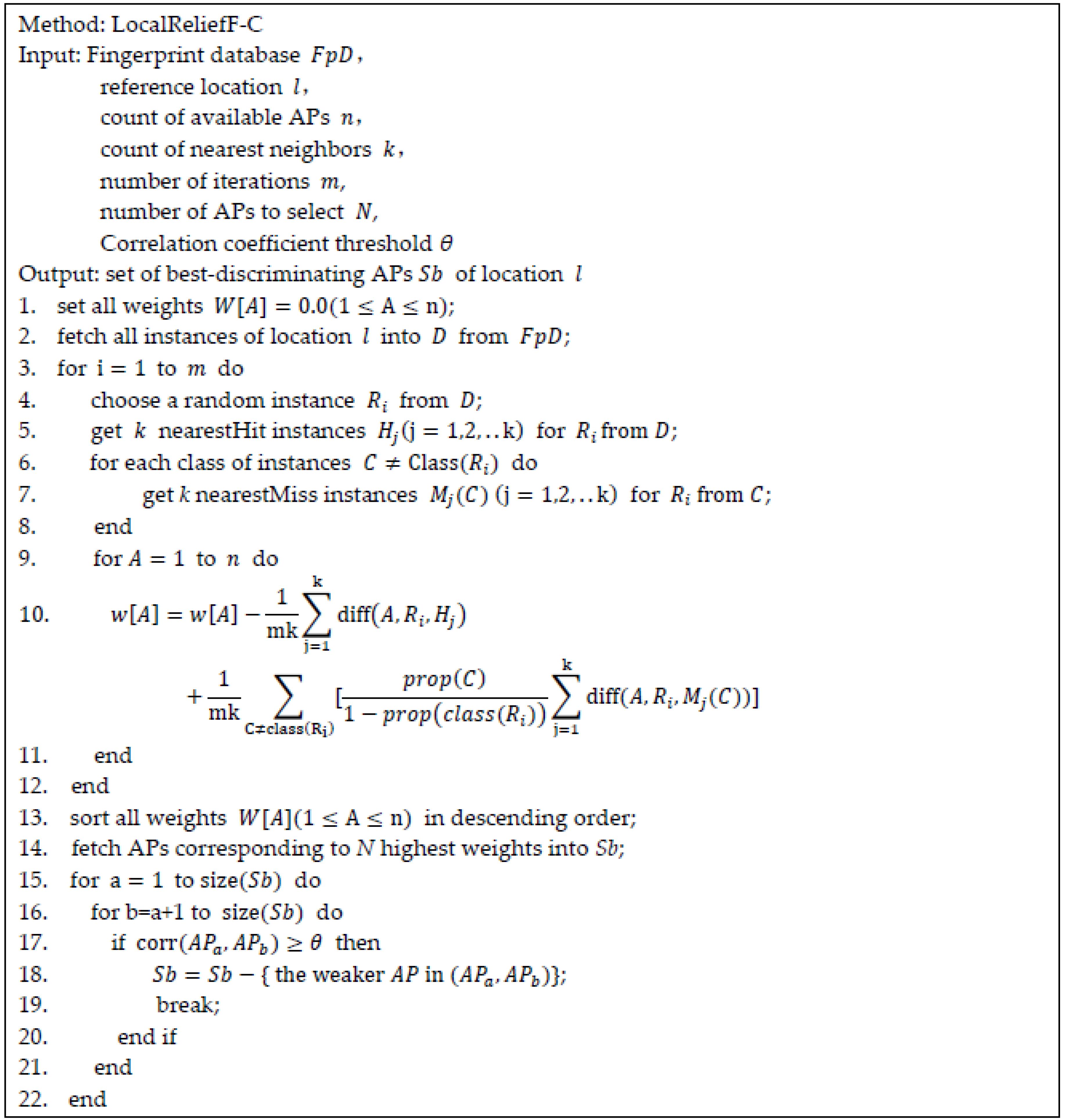Next, it takes into account each different class $C$ and uses the instances proportion $prop\left(C\right)/\left(1-prop\left(class\left(R\_i\right)\right)\right)$ as its contribution factor, where $prop\left(C\right)$ indicates the number of instances of class $C$ divided by the total number of all instances. Finally, it updates feature weights depending on the weighted contribution of all of the nearest hits and nearest misses. The detailed process of ReliefF is given in Figure 1 (Lines 3–14).

One disadvantage of ReliefF is that it will select all of the APs with high positioning capability even though some of them are redundant for each other. Aiming at removing redundant APs and obtaining a set of the best-discriminating APs just sufficient for positioning, we have exploited the Pearson correlation coefficient, which is a measure of the degree of linear dependence between two random variables [22]. It is defined as the covariance of two variables divided by the product of their standard deviations. The formula is as follows:

$$r=\frac{{\sum }_{i=1}^n\left(x_i-Ex\right)\left(y_i-Ey\right)}{\sqrt{{\sum }_{i=1}^n{\left(x-Ex\right)}^2.{\sum }_{i=1}^n{\left(y-Ey\right)}^2}}$$

(3)

The Pearson correlation coefficient ranges between −1 and 1. Given two APs, we calculate $r$, which is the correlation coefficient of their RSS vectors, and compare the absolute value of $r$ with $\theta$, the threshold that we set. If $\left|r\right|$ is greater than $\theta$, it is assumed that the two APs are significantly correlated, namely redundant for each other. Typical values for $\theta$ are given in Section 5.

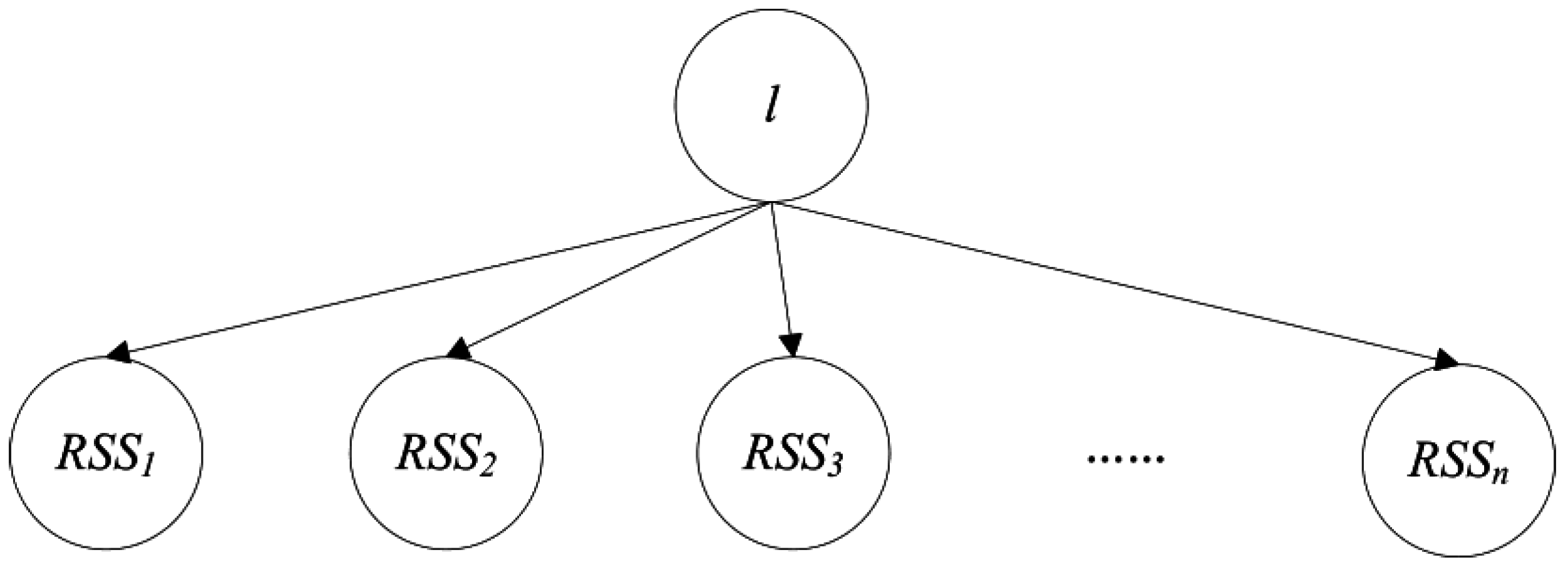
In order to give a detailed description of LocalReliefF-C, the definition of the database is firstly made as follows:

$$FpD=<{\left(l,R\right)}^{\left(i\right)}>,i\in \left\{1,2,\dots ,U\right\}$$

(4)

where ${\left(l,R\right)}^{\left(i\right)}$ represents the i-th instance and U indicates the count of all of the instances; $l$ refers to the reference location, namely the class label of instances; $R=\left[RS{S}_1,RS{S}_2\dots RS{S}_n\right]$, which is an $n$-dimension vector consisting of the received signal strengths from each AP at the reference location $l$; and $n$ refers to the count of available APs. In the machine learning method, each AP is treated as a feature. A weight W is assigned to each AP, which measures its discriminating ability, namely the positioning capacity. The pseudo-code of LocalReliefF-C is displayed in Figure 1. The method firstly calculates the weight for each AP (Lines 1–12), then sorts the weights in a descending order and, finally, retains the N of the APs in the set Sb that correspond to the N highest weights (Lines 13–14). Afterwards, it traverses the set Sb to calculate the correlation coefficients for every two APs and obtains the final set of best-discriminating APs after removing the redundant ones (Lines 15–22).

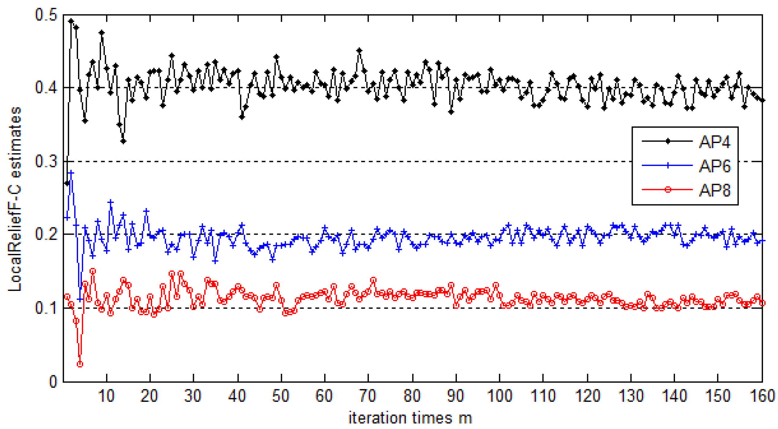
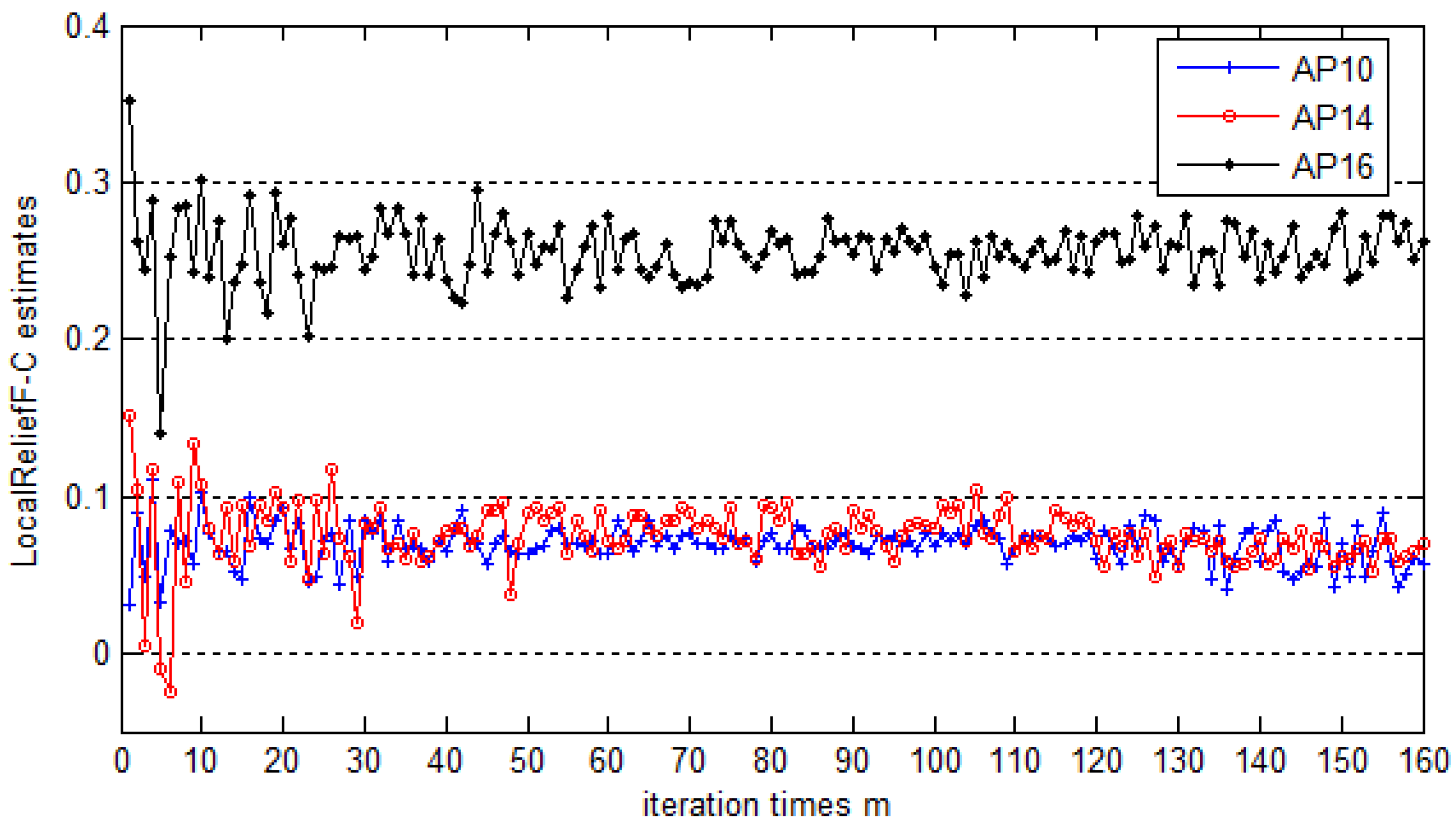
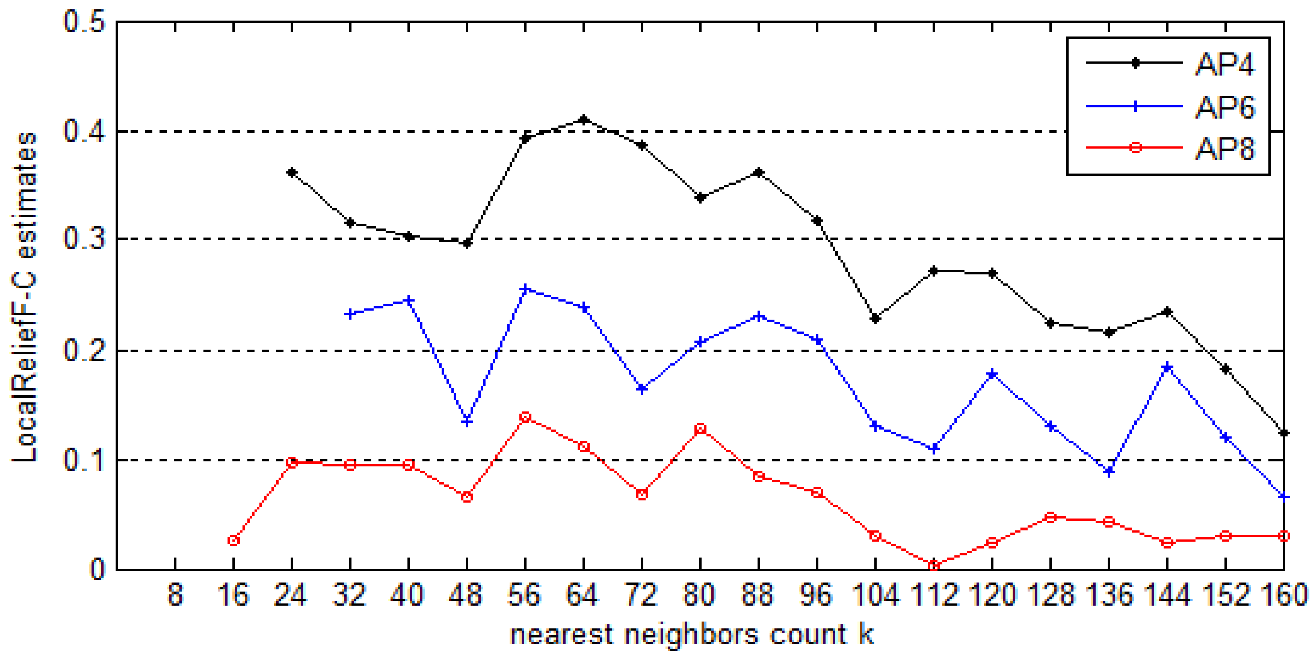
In Figure 1, the parameter k represents the count of nearest neighbors, while m indicates the number of iterations. Usually, estimated weights climb to maximum values when k lies in some proper range and then decrease with the increase of k. In essence, m represents the coverage degree of the instance space for the algorithm. The greater m is, the better the performance is. However, the computational complexity of the algorithm increases with the increase of parameter m. Both of the parameters m and k should be set properly. Their typical values are given in Section 5. 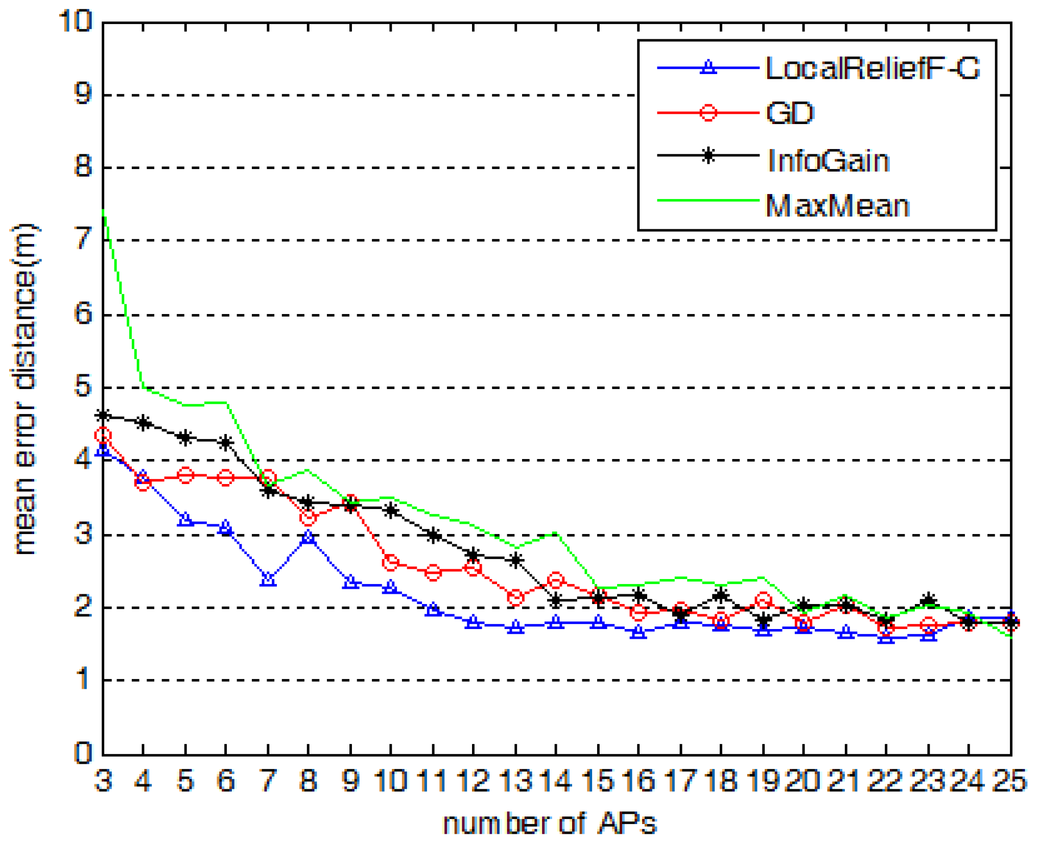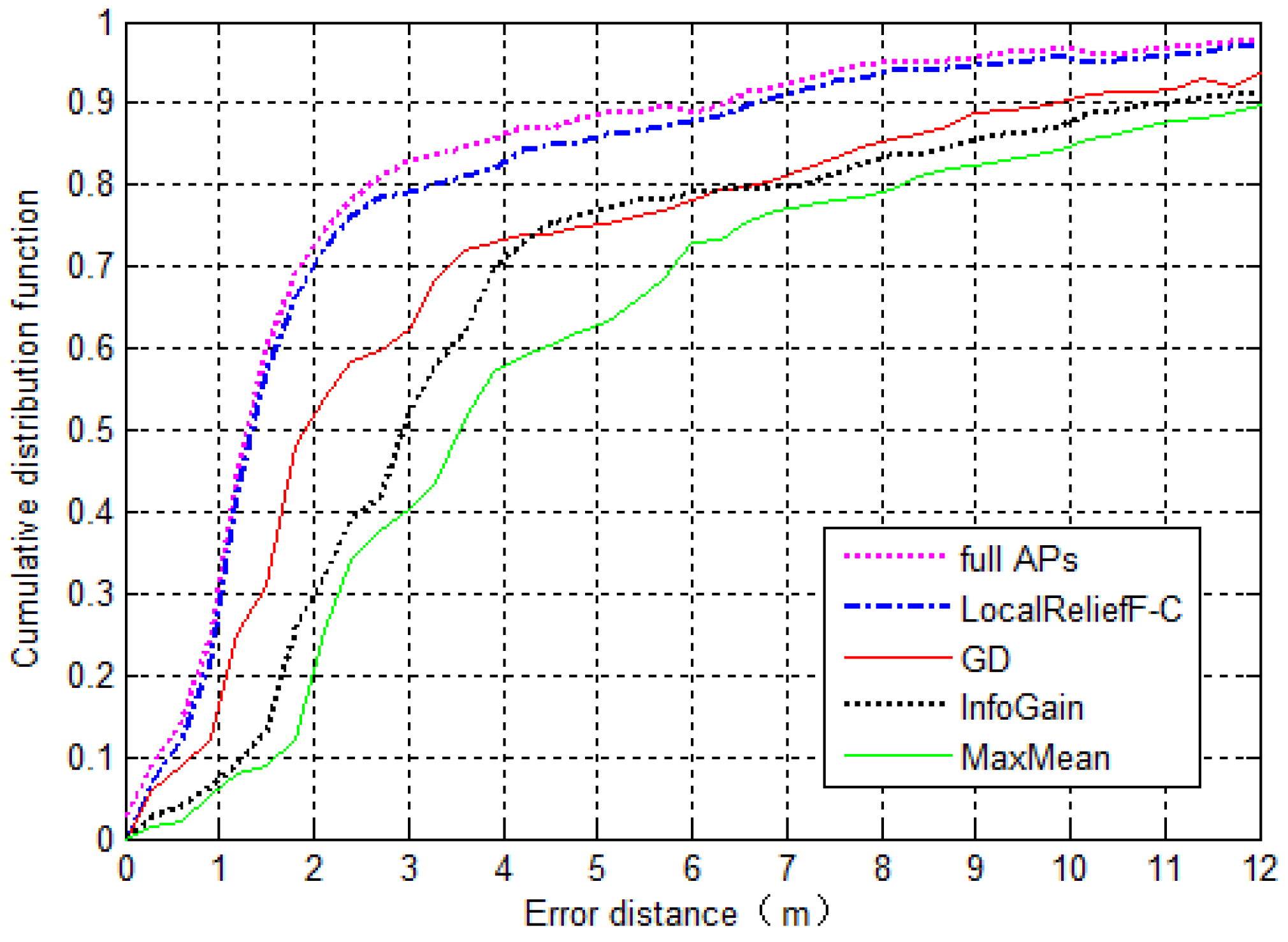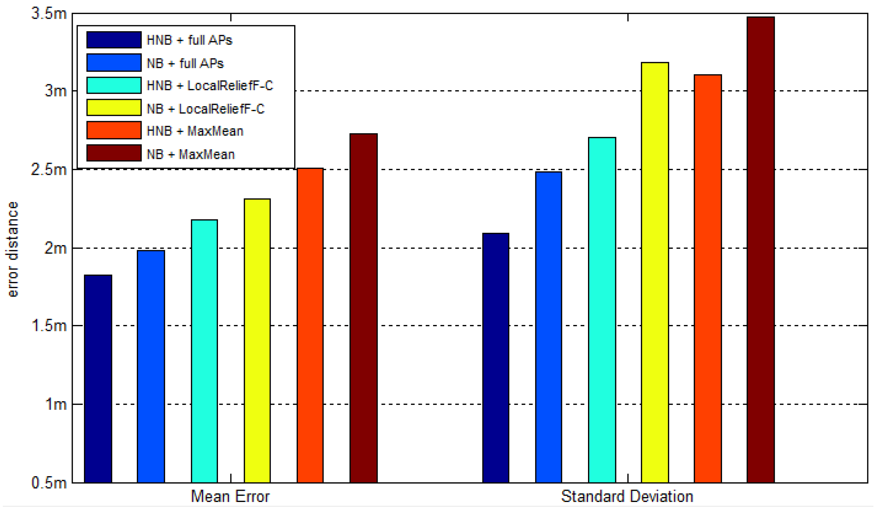The parameter N represents the number of APs to select, which is closely related to the positioning accuracy. Section 5.4 gives the proposed value of N and makes the comparison of positioning accuracy between systems using different AP selection methods. In addition, note that in order to find the k nearest neighbors, we choose the Manhattan distance to measure the distance between two instances. This is defined as the sum of the difference of each feature. Given two instances $R_1\mathrm{and}{R}_2$, their Manhattan distance is calculated as follows:

$$\mathrm{dist}\left(R_1,R_2\right)={\displaystyle \sum }_{\mathrm{A}=1}^{\mathrm{n}}diff\left(A,R_1,R_2\right)$$

(5)

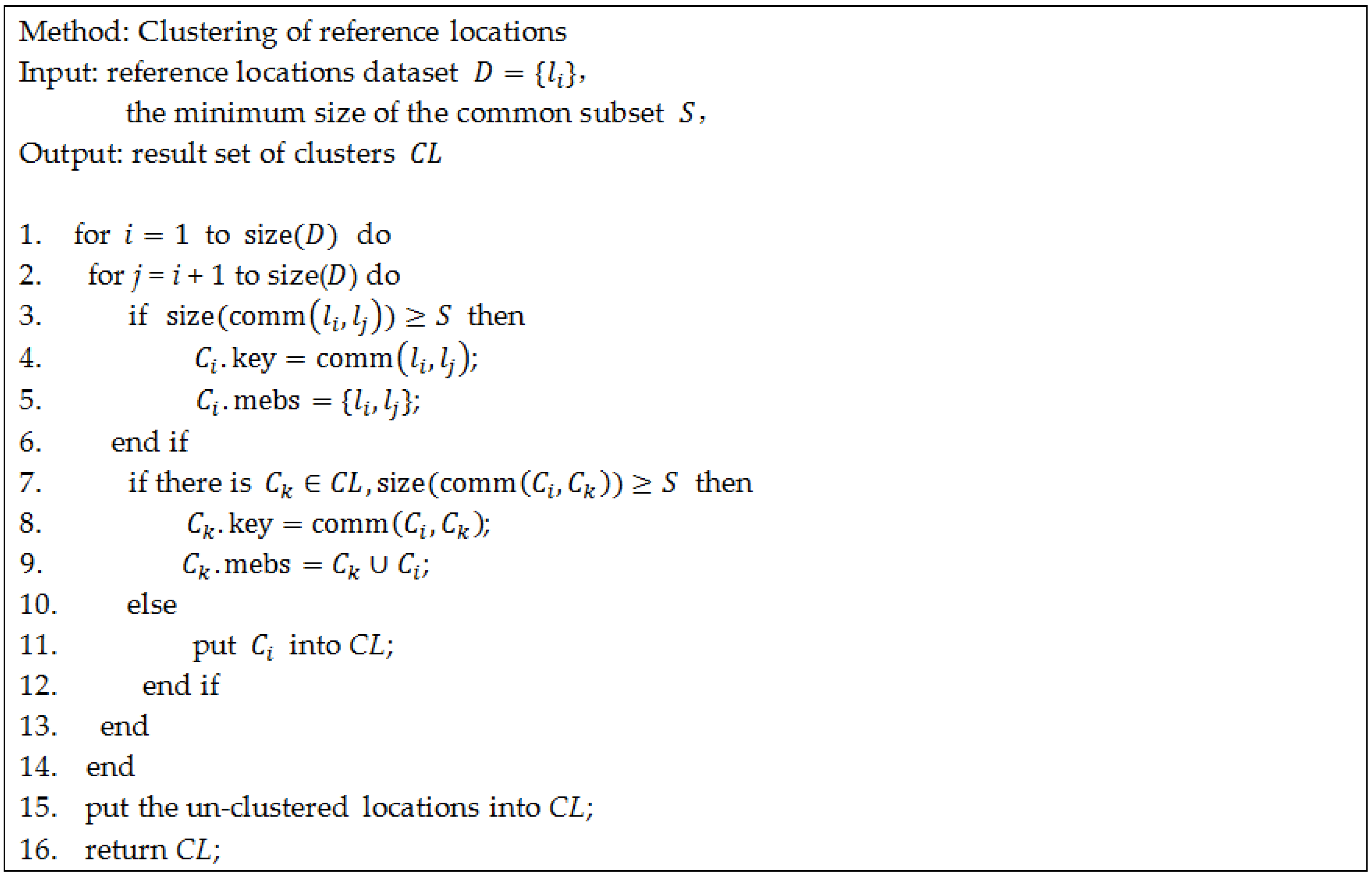
Additionally, we have also utilized the well-known Euclidean distance instead of the Manhattan distance. The result shows that it does not make a significant difference for the sorting result of APs’ weights. Furthermore, another point worth noting is that the sets of best-discriminating APs vary with the reference locations, which is just the same as the situation of the strongest AP set in [16]. In order to get the different sets of best-discriminating APs of reference locations, LocalReliefF-C improves the process of sampling of ReliefF. It randomly chooses samples in a localized instance space corresponding to the given reference location rather than the whole instance space, as shown in Lines 2–4 of Figure 1. This is why the term ‘local’ is added to the name of our proposed method. Afterwards, all of the obtained sets of best-discriminating APs are used as a basis for the following clustering process of reference locations.

3. Clustering of Reference Locations Based on the Common Subsets of Best-Discriminating APs

3.1. Proposed Clustering Method of Reference Locations

As we all know, it is quite time consuming to search the matched location from a great deal of fingerprints in the database. It is necessary to group similar reference locations into clusters. The searching speed can be improved through the process of determining the target cluster for the new RSS sample, firstly, and then estimating the exact location in the cluster. In [19], Chen et al. have done similar work by means of the classical K-means clustering algorithm. They have concentrated more on the data similarity of RSS samples. In our opinion, similar reference locations are those having the common set of best-discriminating APs. Therefore, based on obtaining the set of best-discriminating APs for each reference location, we have introduced a novel overlapping clustering method to group reference locations sharing a common subset of best-discriminating APs into one cluster. Whenever a new cluster is generated, it will search for whether there is an existing cluster that can merge with it. It stops until no new cluster can be generated. It always converges to the same result, which is independent of the processing sequence of the fingerprints and only determined by the obtained subsets of best-discriminating APs of reference locations.

Note that due to the complexity of the real dataset, the set of best-discriminating APs of each reference location tends to be different. Therefore, in practice, a common subset rather than the entire identical set of best-discriminating APs is chosen as the clustering condition. Here, we define a parameter S, which represents the minimum size of the common subset we use. Concretely, the reference locations are grouped into the same cluster if their corresponding sets of best-discriminating APs have no less than S common elements. In this method, the data structure of a cluster consists of two fields. One is “key”, which records the subset of these common APs corresponding to it, and the other is “member list”, which reserves the names of reference locations within it. Figure 2 gives the pseudo-code of the method. The method traverses the reference location dataset D and makes the comparison between every two locations. If the size of the common subset of best-discriminating APs of two locations is equal to or greater than S, both of them are grouped into a new cluster. Subsequently, it searches for whether the result set contains a cluster that can be merged with the new cluster. If it is found, the fields of the member list and the key for the found cluster are updated respectively in order to complete the cluster combination. Otherwise, the new cluster is added into the result set. Finally, all of the reference locations that have not been clustered are added into the result set. Compared with the K-means algorithm, the proposed method has some advantages. First, it requires no complex computational operations. All it needs to do is count and compare the number of common elements of the best-discriminating APs set. K-means needs to calculate the Euclidean distances between each sample and the centroid, which is iterated several times and includes many multiplication operations. Second, the clustering result does not rely on the initial records to process. As for the K-Means algorithm, the clustering result changes with the choice of initial centroid. Additionally, the clustering number k of K-means has to be set at first, which is always a difficult problem to determine. The analysis of the clustering process is given in Section 5.3 based on an experimental example, while the impact of parameter S on clustering performance is also discussed.

3.2. Determining the Target Cluster in the Online Stage

During the offline stage, the fingerprint database has been built; the best-discriminating APs sets for reference locations are obtained; and the clustering of locations has also already been completed. Now, in the online stage, on a certain unknown location $l_x$ when an RSS instance, or a sequence of them, is given, the first step is to determine the target cluster. It is worth noting that the reference location is actually covered by a grid of 2 m × 2 m square, as mentioned in Section 5, where the experimental setup is introduced. Namely, all RSS instances that are obtained when the observer stays within this grid can be used as members of the instance sequence of this reference location. The process consists of two steps: calculation of the best-discriminating AP set of location $l_x$ and comparison between this set and each cluster key in the fingerprint database.

Concretely, we define $D_x$ as the set of RSS instances of location $l_x$, $S{b}_x$ as the best-discriminating AP set of location $l$ and $CL=<C_i>,i\in \left\{1,2,\dots \right\}$ as the reference location clusters set in the fingerprint database, among which $D_x$ and $CL$ are given. In the first step, in order to calculate $S{b}_x$, we apply the proposed AP selection method LocalReliefF-C to $D_x$. All of the operations are similar, but there are still some differences worthy of explanation. First, during the process of calculating the weights of the APs, we take $D_x$ as a class and each cluster of $CL$ rather than each reference location as a different class. As mentioned above, it is required to find the nearest neighbors in each different class. Since the number of clusters is usually much smaller than the number of reference points, this process can cost less time than the offline stage. Second, if the size of a given $D_x$ is small, or even equal to one, the calculation process can still be accomplished when the nearest neighbors of different classes contribute more to the weight calculation. If there is only one instance in $D_x$, the process of finding nearest neighbors in the same class is omitted, and the calculating formula at Line 10 of Figure 1 changes to:

$$w\left[A\right]=w\left[A\right]+\frac{1}{\mathrm{mk}}{\displaystyle \sum }_{\mathrm{C}\ne \mathrm{class}\left({\mathrm{R}}_{\mathrm{i}}\right)}[\frac{prop\left(C\right)}{1-prop\left(class\left(R_i\right)\right)}{\displaystyle \sum }_{\mathrm{j}=1}^{\mathrm{k}}\mathrm{diff}\left(A,R_i,M_j\left(C\right)\right)]$$

In the second step, we compare $S{b}_x$ with the key of each cluster $C_i$ and record the counts of the common APs that they have. Finally, the cluster corresponding to the largest count is the target. Namely, we want $C$, which can maximize $\mathrm{size}\left(\mathrm{comm}\left(C_i,S{b}_x\right)\right)$. For example, assuming we are given the calculated $S{b}_x$= [AP3, AP4, AP5, AP7], $C_1.\mathrm{key}=\left[\mathrm{AP}2,\mathrm{AP}4,\mathrm{AP}6,\mathrm{AP}11\right]$ and $C_2.\mathrm{key}=\left[\mathrm{AP}3,\mathrm{AP}5,\mathrm{AP}7\right]$, then the common AP counts of them are, respectively, one and three. In this situation, $C_2$ is the target cluster. The process of determining the target cluster is illustrated in Figure 3. When the target cluster is identified, the following work is to estimate the location in the cluster.

4. Location Estimation Exploiting Mutual Influences of Access Points

4.1. Classic Location Estimation Method of Naive Bayes

In order to estimate the target location in the given cluster, recent researchers utilize the naive Bayes classifier, which has also been widely used in data mining and machine learning fields. Based on a solid mathematical theory, naive Bayes is simple to implement and can achieve good performance in most cases [25,26]. Its structure is shown in Figure 4, in which the class node l is the parent of all of the feature nodes. As the simplest form of Bayes network classifier, naive Bayes naively assumes that all of the features are independent of each other. In terms of the indoor positioning problem, the class node l represents the location, and the feature node RSS_i corresponds to the signal strength received from each AP.

The core idea is the maximum a posteriori estimation. Concretely, for a mobile object on a certain unknown location, given the observation of signal strength vector $R=\left[RS{S}_1,RS{S}_2\dots RS{S}_n\right]$, the location $l$ that maximizes the posterior probability $P(l|R)$ is the target position we want. That is, to obtain:

$${\mathrm{argmax}}_l\left(P\left(l|R\right)\right)$$

(6)

In this situation, $P\left(R\right)$ and $P\left(l\right)$ are constant. As described in [16], Equation (6) is transformed as follows:

$$\begin{gathered} {\mathrm{argmax}}_l\left(P\left(l|R\right)\right)={\mathrm{argmax}}_l\left[\frac{P\left(R|l\right)\cdot P\left(l\right)}{P\left(R\right)}\right] \\ ={\mathrm{argmax}}_l\left[P\left(R|l\right)\right] \\ ={\mathrm{argmax}}_l\left[{\displaystyle \prod }_{i=1}^{n}P(RS{S}_i|l)\right] \end{gathered}$$

(7)

In practice, each $P(RS{S}_i|l)$ can be calculated by the aid of the distribution function of the signal strength, which is estimated from the instances of the fingerprinting database.

4.2. Proposed Location Estimation Method of Hidden Naive Bayes

The basic assumption of the naive Bayes location estimation method is that the APs are conditionally independent and have no impact on each other [27,28]. Such an assumption is too ideal and inconsistent with the real environment. As we all know, in real WLAN environment received signals from different APs are inevitably interfering with each other due to their overlapping transmission channels.

Hidden naive Bayes (HNB) is an improved classifier for naive Bayes, which requires no assumption of conditional independence between features and takes into account the impact between the features to improve the classification accuracy [29,30]. This paper introduces HNB into the indoor positioning field, which can depict the real WLAN environment more accurately and improves the positioning accuracy via exploiting the interaction between APs.

HNB defines a hidden parent node for each feature to combine the impact of the other features. As shown in Figure 5, each feature node $RS{S}_i$ has a hidden parent node $RS{S}_{hpi}$, $i\in \left\{1,2,\dots ,n\right\}$, which is depicted as a dashed circle. The arrow from $RS{S}_{hpi}$ to $RS{S}_i$ is also a dashed line, which indicates the hidden parent-child relationship.

Look back at Equation (7), in order to determine the target position, we want:

$$\begin{array}{ll}\hfill {\mathrm{argmax}}_l\left(P\left(l|R\right)\right)& ={\mathrm{argmax}}_l\left[P\left(R|l\right)·P\left(l\right)\right]\hfill \\ & ={\mathrm{argmax}}_l\left[P\left(Rl\right)\right]\hfill \\ & ={\mathrm{argmax}}_l\left[P\left(RS{S}_1,\dots ,RS{S}_n,l\right)\right]\hfill \end{array}$$

(8)

Here is the key point: in the HNB model, the joint probability distribution in Equation (8) is defined as:

$$P\left(RS{S}_1,\dots ,RS{S}_n,l\right)=P\left(l\right){\displaystyle \prod }_{i=1}^{n}P\left(RS{S}_i|RS{S}_{hpi},l\right)$$

(9)

where:

$$P\left(RS{S}_i|RS{S}_{hpi},l\right)={\displaystyle \sum }_{j=1,j\ne i}^n{W}_{i,j}*P\left(RS{S}_i|RS{S}_j,l\right)$$

(10)

In Equation (10), there is ${\sum }_{j=1,j\ne i}^n{W}_{i,j}=1$. Actually, the parent node ${\mathrm{RSS}}_{hpi}$ is the weighted sum of the impact on ${\mathrm{RSS}}_i$ from the rest of the feature nodes. The weight $W_{i,j}$ is defined as:

$$w_{i,j}=\frac{I\left(RS{S}_i;RS{S}_j|l\right)}{{\sum }_{j=1,j\ne i}^{n}I\left(RS{S}_i;RS{S}_j|l\right)}$$

(11)

where:

$$\mathrm{I}\left(\left(RS{S}_i;RS{S}_j|l\right)\right)={\displaystyle \sum }P\left(RS{S}_i,RS{S}_j,l\right)log\frac{P(RS{S}_i,RS{S}_j|l)}{P(RS{S}_i|l)P(RS{S}_j|l)}$$

(12)

$I\left(RS{S}_i;RS{S}_j|l\right)$ is the conditional mutual information between the feature $RS{S}_i$ and $RS{S}_j$. Under the assumption that l is known, it measures how much the uncertainty of $RS{S}_i$ will reduce when the value of $RS{S}_j$ is known. All of the probability in the equation can be calculated by the corresponding distribution function, which is estimated from the training instances in the fingerprint database via a histogram estimator. These distribution functions can also be obtained through other nonparametric techniques, such as kernel density estimation. Finally, through calculation and comparison, the location that maximizes the joint probability in Equation (8) is the result that we want.

5. Experiments and Analysis

5.1. Experimental Setup

In order to evaluate the proposed strategies, we have conducted the experiments on the fourth floor of the School of Environmental Science and Spatial Informatics at the China University of Mining and Technology (CUMT). It is a typical office environment with a total area of about 800 square meters, including a few offices, conference rooms and several halls. Figure 6 depicts the layout of the experimental environment. Nearly 50 APs can be detected throughout the entire environment, which include the existing APs for network services located on different floors and some others we have deployed specially to verify the effectiveness of the AP selection method. The whole floor is modeled as a space of 180 reference locations, each of which covers a 2-m grid cell. On average, each position is covered by 25 APs.

Utilizing the self-developed app running on an Android 4.4-powered Huawei (ShenZhen, GuangDong, China) smart phone, which is equipped with quad-core 1.3 GHz and 1 GB ram, we have collected 160 RSS samples from all of the surrounding APs at each reference location. Considering that the sample signal strengths are time variant and easily affected by the surrounding environments, the sample acquisitions are done at different times, 9:00 a.m. and 3:00 p.m., respectively, on two different days. At each time of the sample acquisition process, the observer holding the smart phone faces the four directions of east, south, west and north, in turn, and collects 10 samples toward each direction. The raw data are collected in a text file, which consists of several fields, such as reference location, SSID (service set identifier) of the AP, MAC (medium access control) address of the AP and signal strength. Before any operations, the pre-processing unit we developed completes the task of transforming the raw data into the fingerprint records in database. For simplicity, APs are identified by subscripted numbers, which are converted from the combination of SSID and MAC address. The partial segments of the raw data and the fingerprint records are respectively displayed in

Table 2. Raw data collected.

SSID	MAC Address	Signal Strength	Reference Location
CMCC(China Mobile Communications Corporation)-EDU	00:60:b3:c9:fa:ae	−63	@1
ChinaNet	80:f6:2e:1b:e2:20	−90	@1
CMCC-EDU-CUMT	06:60:b3:c9:fa:ae	−70	@1
TP-LINK(name of a network equipments supplier)_927D4A	6c:e8:73:92:7d:4a	−74	@1
TP-LINK_9199E4	6c:e8:73:91:99:e4	−60	@1
….	…..	…	…

and

Table 3. Fingerprint records.

Reference Location	AP1	AP2	AP3	AP4	AP5	…
@1	−63	−90	−70	−74	−60	…
@1	−62	−87	−66	−78	−53	…
@1	−70	−77	−62	−80	−55	…
@1	−74	−80	−69	−68	−48	…
@1	−60	−83	−58	−70	−50	…
	…	…	…	….	…	…

.

5.2. Parameter Tuning of the LocalReliefF-C AP Selection Method

As mentioned in Section 2.2, the parameter m indicates the iteration times when calculating the classification weights of APs of LocalReliefF-C. It can be found that with the increase of m, the reliability of the weight result is stronger, but the computation complexity is also increased. Therefore, a tradeoff needs to be made between the positioning performance and the computation overhead. Concretely, the optimal value of m is hoped to be as low as possible, and meanwhile, it can ensure the good estimated results of AP weight. This is problem-dependent and related to the dataset with which we deal. The process of parameter tuning is made as follows.

We randomly choose several reference locations and calculate the weights of different APs when different values of m are adopted. Figure 7 depicts a representative example, in which the result is based on reference Location 1 and APs AP4, AP6 and AP8. Figure 8 shows that the estimated weights of these APs change with the iteration time m. It can be found that the estimated weights of AP4, AP6 and AP8 fluctuate seriously when 1–30 iterations are used. After 40–60 iterations, the weights almost become stable. Furthermore, a better result cannot be obtained even though many more iterations are adopted. Therefore, 40 is our ideal choice for m, which is far less than 160, the maximum value for m. This also indicates that the proposed method has good scalability and can handle large datasets. Additionally, the consistent results are obtained in empirical analysis at another reference location 12, as shown in Figure 8, where three APs, AP10, AP14 and AP16, are randomly chosen.

The parameter k represents the number of the nearest neighbor instances when calculating the classification weights of APs in LocalReliefF-C. Note that only one nearest neighbor is used in the original algorithm of Relief. Inevitably, there are redundant and noisy features in real datasets, which interferes with finding the nearest neighbor and causes unreliable estimation results. In order to cope with this problem, Kononenko extends the number of nearest neighbors to k and suggests that the default value of k is 10 [23]. Even so, it is assumed that the choice of k is also closely related to the problem complexity. Under the premise of m being equal to 40, we have done the test and found that for our dataset, the weights usually reach the maximum values when k lies in the range of 55–65 and then decrease with the increase of k. Figure 9 shows an example of the estimated weight change of AP4, AP6 and AP8 with the values of k at reference Location 1. The reason why weights decrease as k gets higher is that the probability of positive and negative updates in the weight calculation formula is more likely equal when more nearest neighbors are obtained. Usually, for a certain AP, a higher weight is desired, which lowers the probability to ignore an important AP. Therefore, for our dataset, 60 is selected as the optimal value of k, which guarantees that higher AP weights are obtained.

The parameter $\theta$ is the threshold of the Pearson correlation coefficient used to remove the redundant APs in LocalReliefF-C. The calculated value of the Pearson correlation coefficient, denoted as $r$, describes the linear correlation between two APs. The value of $r$ lies in $\left[-1,1\right]$. $0<r<1$ implies a positive correlation, and $-1<r<0$ implies a negative correlation. As an auxiliary tool for correlation analysis, the scatterplots can intuitively reflect the correlation of two features. Figure 10 depicts the scatter plots drawn from our experimental data, in which (a) shows the positive correlation and (b) shows the negative correlation. Figure 10a shows the scatter plots of AP8 and AP9 at reference Location 1, with r = 0.89. Figure 10b displays the scatter plots of AP3 and AP17 at reference Location 2, with r = −0.75. Usually, drawing scatter plots is helpful to find the correlation trend of two APs. Note that scatterplots are only important and drawn in the data analysis phase. Once the correlation rank of APs is found, it is not needed to draw scatterplots in the phase of calculating the correlation coefficient value.

It has been pointed out that correlated degree of two APs increases with the increase of the absolute value $\left|r\right|$ [22]. Through the correlation analysis and hypothesis test on our dataset, it is concluded that the correlation degree is generally low or moderate when $\left|r\right|$ lies between 0 and 0.59. When $\left|r\right|$ is greater than 0.6, the correlation degree is significant. We choose 0.6 as the value of the threshold $\theta$. If the absolute value of the Pearson correlation coefficient of two APs exceeds $\theta$, it is assumed that they are significantly correlated, namely redundant for each other. Generally, in order to preserve more useful information, the weaker AP of them is removed, and the stronger is reserved. For example, the set of APs at reference Location 1 is {AP2, AP9, AP11, AP4, AP6, AP17, AP13, AP10, AP7, AP19}, which is sorted by the classification weight in descending order. The Pearson correlation coefficients of different APs in the set are, respectively, calculated, which is shown in

Table 4. Pearson correlation coefficients of different APs at reference Location 1.

	AP2	AP9	AP11	AP4	AP6	AP17	AP13	AP10	AP7	AP19
AP2	1	0.11	−0.28	0.09	−0.17	0.21	0.06	0.32	0.41	0.13
AP9		1	0.15	−0.2	−0.25	0.11	0.79	0.04	0.09	−0.08
AP11			1	0.07	0.06	−0.3	0.16	0.88	0.80	−0.34
AP4				1	−0.27	0.43	−0.16	0.29	0.31	0.49
AP6					1	−0.58	−0.25	0.12	0.04	−0.24
AP17						1	0.17	0.09	−0.2	0.25
AP13							1	0.05	0.09	−0.15
AP10								1	0.89	−0.23
AP7									1	−0.17
AP19										1

. It can be found that there are four pairs of highly-correlated APs: AP9 and AP13, with r = 0.79; AP11 and AP10, with r = 0.88; AP10 and AP7, with r = 0.89; and AP11 and AP7, with r = 0.80. After removing all of the redundant APs, the final set of best-discriminating APs is {AP2, AP4, AP6, AP9, AP11, AP17, AP19}. In a similar way, the set of best-discriminating APs at each reference location can be obtained.

5.3. Experimental Analysis of the Clustering of Reference Locations Based on the Common Subsets of Best-Discriminating Aps

The parameter S is crucial for the performance of reference location clustering based on the common subsets of best-discriminating Aps. To be clearer, an experimental illustration is given.

Table 5. Sets of best-discriminating APs of reference locations.

Reference Location	Sets of Best-Discriminating APs
@1	AP2, AP4, AP6, AP9, AP11, AP17, AP19
@2	AP3, AP5, AP7, AP8
@3	AP2, AP4, AP6, AP11, AP16
@4	AP3, AP5, AP7, AP14
@5	AP2, AP4, AP6, AP11, AP25
@6	AP7, AP13, AP18
@7	AP3, AP5, AP8, AP12
@8	AP19, AP21
@9	AP7, AP13, AP22

displays the clustering dataset extracted from our experimental dataset, which contains nine reference locations with the corresponding sets of best-discriminating APs. The records are processed from @1–@9 and the clustering results are depicted in Figure 11 and Figure 12. There are two data fields of each cluster: “Key” and “Mebs”. The Key field records the common subset of APs, while the Mebs field records all members of reference locations in the cluster. There are six and four clusters obtained, when the parameter S is set to three and two, respectively. Note that in Figure 11, the clusters No. 2 and No. 3 cannot be combined into one cluster even though they have a common subset {AP3, AP5}. The reason is that the size of the common subset equals two, which is less than three, the value of S. However, in Figure 12, the two clusters are merged when S is set to two.

Additionally, it is found that we obtain the same clusters when the locations are scanned in a different order, for example, from Locations @9–@1. This is because, for the proposed method, the similarity of locations is just measured by the common subset of the best-discriminating Aps, and the condition to group locations into one cluster is the number of their common subset of best-discriminating APs that exceeds parameter S. The clustering process is only determined by the dataset itself and the parameter S, which is not affected by the choice of the first fingerprint to process or the processing sequence of fingerprints. Therefore, as for a given dataset, it always converges to the same result once the parameter S is set.

Table 6. Effect of S on the count and the average size of clusters.

S	Count of Clusters	Average Size of Clusters
1	4	2.75
2	4	2.25
3	6	1.67
4	7	1.3
5	9	1

shows the effect of S on the count and average size of clusters. It can be found that with the increase of S, the count of the clusters increases, whereas the average size of the clusters decreases. Too high or too low a value of the size and count is undesirable, which can reduce the performance of clustering. In fact, the selection of S is problem-dependent and determined by the dataset we deal with. The optimal value of S should guarantee that the average size and total number of clusters are appropriate relative to the scale of the problem. As for our experiment dataset, we have set S = 6 and obtained 10 clusters.

5.4. Accuracy and Precision Comparison of Different AP Selection Methods

This section focuses on the effect of the proposed AP selection method on the positioning performance. LocalReliefF-C is compared with other existing methods of AP selection, such as GD (group-discrimination), InfoGain and MaxMean. The proper value of the parameter N in LocalReliefF-C, that is the number of APs to use, is also given. As described in Section 2, the method of GD measures the positioning capabilities for groups of APs by means of the risk function from support vector machines (SVM). Furthermore, the InfoGain method makes the AP selection by calculating the information gain for each AP, whereas the MaxMean method selects the APs with the highest average signal strength.

All of those methods have been implemented on our pre-collected fingerprints database to complete AP selection. From all of the 180 reference locations, we have chosen 120 of them as test locations, which can almost cover every part of the experimental area. We have collected 80 observed samples on each reference location for the online location estimator. For each of the methods, only the signal strengths of its corresponding selected APs are taken as the input for the location estimator. Considering that the signal is time variant, samples and training samples are collected on different days. For simplicity, we choose the naive Bayes classifier as the location estimator in the online stage. In order to compare the performance of various methods, we have used three metrics: error distance, accuracy and precision. The error distance is the Euclidean distance between the estimated result and its actual coordinates. Assuming that, at a certain test location, its corresponding coordinates are $\left(x_i,y_i\right)$ and the estimated result is $\left(X,Y\right)$, then the error distance is defined as $\sqrt{{\left(x_i-X\right)}^2+{\left(y_i-Y\right)}^2}$. The accuracy is one of the most important performance metrics for a positioning system, which is described as the mean error distance of all test locations. The lower the mean error distance, the higher the accuracy of the method. Precision is another metric of positioning performance, which is usually described as the cumulative distribution function (CDF) of the error distance. In order to compare accuracy, the number of selected APs has been set from 3–25, and the average values of error distances on 180 test locations have been correspondingly calculated and reserved. The result is shown in Figure 13. The comparison result of precision is shown in Figure 14.

Figure 13 depicts the mean error distances versus the number of the APs for those AP selection methods. It can be found that the mean error distances of each method decline with the increase in the number of APs. However, compared with other methods, the curve of LocalReliefF-C is relatively flat, and all of the values of the mean error distance stay low. This is because LocalReliefF-C selects the APs with the best discriminating capability and moreover removes the redundant ones. Those selected APs contain more valuable information for location estimation. Hence, LocalReliefF-C can obtain the comparable performance as those methods using more APs. Since the method uses fewer APs, the computational cost of the system is reduced, and the efficiency is improved. This also proves the necessity and significance of the research on the method of AP selection. Additionally, note that for LocalReliefF-C, when the number of APs is greater than 12, the mean error distance almost stops decreasing and maintains a stable value of about 1.8 meters. Even though many more APs are used, the accuracy cannot be improved. Therefore, in view of the real data we deal with, the optimal value of parameter N in LocalRelief-C can be 12. In addition to the number of APs, the accuracy of positioning systems is also closely related to the location estimation method. The next section describes the experimental analysis on the accuracy improvement of a novel location estimation method that utilizes the HNB model instead of the NB model.

In addition to the three AP selection methods above, during the precision comparison process, we have added one more methods called “full APs”. As for our dataset, it utilizes the full set of 25 detectable APs in location estimation. Other methods of AP selection choose the 12 best APs to use according to their selection principles, respectively. CDF curves of the error distances between them are drawn and compared in Figure 14. It can be found that LocalReliefF-C outperforms the other three AP selection methods and basically achieves a comparable performance as the method using the full set of APs. The curve of LocalReliefF-C climbs to the top at a faster rate, which indicates that the error distance is concentrated in a smaller range. Concretely, for LocalReliefF-C, the probability of the error distance within four meters is 82%, whereas the corresponding results of the other three methods are 73%, 70% and 59%, respectively. It is improved by 9%, 12% and 24%, respectively. This validates the effectiveness of the proposed AP selection method.

5.5. Precision Comparison of Different Location Estimation Methods

In order to evaluate the performance of the proposed location estimation method of hidden naive Bayes, the two models of location estimation, HNB and NB, and the two methods of AP selection, LocalReliefF-C and MaxMean, are respectively combined into positioning systems. To obtain the best performance, the number of selected APs is set to 12. For comparison, the two models using full APs are also included. Finally, a total of six types of positioning systems are tested on the same experimental dataset, which are HNB + full APs, NB + full APs, HNB + LocalReliefF-C, NB + LocalReliefF-C, HNB + MaxMean and NB + MaxMean. The CDFs of the error distance of all of the systems are depicted in Figure 15.

It can be found that HNB outperforms NB, no matter which AP selection method is used. The probability of the error distance within three meters and five meters is improved by 7% and 6% than NB, when the AP selection method of LocalReliefF-C is used. The consistent result is obtained when the AP selection method of MaxMean is used. The probability of the error distance within three meters and five meters is improved, respectively, by 8% and 10% than NB. When full APs are used, it improves 4% and 3%, respectively. Such an improvement results from the good mechanisms of the HNB model: that is, breaking the unrealistic assumption of the conditional independence of APs and exploiting the mutual influence of APs in the process of location estimation. The mean error distance and standard deviation of the positioning systems are reduced when the HNB model is adopted, which can be found from the statistical results in

Table 7. Mean error distance and standard deviation of the four systems.

	HNB + full APs	NB + full APs	HNB + LocalReliefF-C	NB + LocalReliefF-C	HNB + MaxMean	NB + MaxMean
Mean error	1.32	1.48	1.68	1.81	2.01	2.23
Standard Deviation	1.59	1.98	2.21	2.68	2.60	2.97

. The corresponding error bars are shown in Figure 16. This is also a testament to the validity of the HNB model.

5.6. Computational Cost Comparison in the Online Stage

As we all know, it is of significance to lower the computational cost of online location estimation, which can improve the system response speed and enhance the users’ experiences. In order to test the effectiveness of our proposed strategy of AP selection and location clustering on reducing the online computational cost, we have carried out two kinds of online positioning procedures: the first kind uses the full set of APs without clustering, and the second kind uses the selected APs by LocalReliefF-C with location clustering. For comparison, each kind of procedure, respectively, utilizes both estimation models, NB and HNB. The computational cost is measured as the average count of multiplication operations used by each test location estimation. Concretely, we have estimated locations of all 120 test points to calculate the sum of the used multiplication operations and then divided it by 120 to get the average value. The number of the full set of APs is 25, which is the average number of detectable APs on all locations. For LocalReliefF-C, the number of selected APs N is 12, which can guarantee the competitive positioning performance as using full APs. There are, in total, 10 clusters in the fingerprint dataset, and the average size of a single cluster is 18. Figure 17 depicts the computational cost comparison result of the two types of procedures. It can be found that no matter which estimation model is utilized, the computational cost of the positioning procedure is reduced by almost an order of magnitude when using selected APs with clustering.

This is because the clustering strategy makes the search range of the whole fingerprint database shrink to a certain cluster, which reduces the number of comparing and matching operations. Furthermore, AP selection reduces the number of used APs, which can lower the number of multiplications in each record matching. Specifically, for a single test location, the first kind has to make 180 comparisons corresponding to all fingerprints, and the second kind only makes, more or less, 20 comparisons in a cluster based on several key matching operations to determine the target cluster. Additionally, during each record matching, the first kind requires calculating the product of the distribution probability of 25 Aps, whereas the second kind requires that of about 12 APs. Additionally, the procedures using HNB cost more because the mutual information of each pair of APs has to be calculated.

6. Conclusions and Future Work

In this paper, we have presented a novel AP selection method for WLAN fingerprinting positioning, LocalRelief-C, which is inspired by the idea of the feature selection technique and Pearson correlation coefficient. First of all, the importance of APs is ranked according to their classification capability. Then, the redundant APs are determined and removed via the calculation of the Pearson correlation coefficient between them. Eventually, the set of best-discriminating APs is obtained, which contains the most effective APs for the discrimination of locations. The experimental results indicate that the proposed method of LocalRelief-C can ensure that the positioning system achieves a comparable performance as a method that uses many more APs. Subsequently, the reference locations are clustered according to the common subset of best-discriminating APs of each reference location, in order to narrow the search space and improve the positioning speed. In the online stage, the target cluster is determined through comparing the key of each cluster with the set of best-discriminating APs of the RSS observation sequence on this location. During the location estimation stage, the hidden naive Bayes (HNB) model is adopted to take into account the impact between APs. It is believed that the model is more in line with the real WLAN environment and, hence, achieves higher positioning accuracy than naive Bayes. Through the experiments using real data collected in an office environment, the optimal suggested values of the parameters are discussed, and the effectiveness of the proposed methods is validated.

One of our ongoing efforts is to utilize fewer training instances to build a novel model for positioning, which can depict the wireless signals more accurately. Additionally, how to fuse Wi-Fi signals with other available sensor signals, such as accelerometers, gyroscopes and magnetometers, to improve the positioning performance is also being studied.

References

1. Li, X.; Wang, J.; Liu, C.; Zhang, L.; Li, Z. Integrated WiFi/PDR/smartphone using an adaptive system noise extended Kalman filter algorithm for indoor localization. ISPRS Int. J. Geo-Inf. 2016, 5, 8. [Google Scholar] [CrossRef]
2. Jiang, P.; Zhang, Y.Z.; Fu, W.Y.; Liu, H.Y.; Su, X.L. Indoor mobile localization based on Wi-Fi fingerprint’s important access point. Int. J. Distrib. Sens. Netw. 2015, 2005, 1–8. [Google Scholar] [CrossRef]
3. He, S.N.; Chan, S.H.G. Wi-Fi fingerprint-based indoor positioning: Recent advances and comparisons. IEEE Commun. Surv. Tutor. 2016, 18, 466–490. [Google Scholar] [CrossRef]
4. Liu, H.B.; Yang, J.; Sidhom, S.; Wang, Y.; Chen, Y.Y.; Ye, F. Accurate WiFi Based Localization for Smartphones Using Peer Assistance. IEEE Trans. Mob. Comput. 2014, 13, 2199–2214. [Google Scholar] [CrossRef]
5. Huang, C.-C.; Hung-Nguyen, M. RSS-based indoor positioning based on multi-dimensional Kernel Modeling and weighted average tracking. IEEE Sens. J. 2016, 16, 3231–3245. [Google Scholar] [CrossRef]
6. Liu, H.; Darabi, H.; Banerjee, P.; Liu, J. Survey of wireless indoor positioning techniques and systems. IEEE Trans. Syst. Man Cybern. C 2007, 37, 1067–1080. [Google Scholar] [CrossRef]
7. Koyuncu, H.; Yang, S.H.; Koyuncu, H.; Yang, S.H. In A survey of indoor positioning and object locating systems. IJCSNS Int. J. Comput. Sci. Netw. Secur. 2010, 10, 121–128. [Google Scholar]
8. Chai, X.Y.; Yang, Q. Reducing the calibration effort for probabilistic indoor location estimation. IEEE Trans. Mob. Comput. 2007, 6, 649–662. [Google Scholar] [CrossRef]
9. Bahl, P.; Padmanabhan, V.N. RADAR: An in-Building RF-Based User Location and Tracking System. In Proceedings of the 19th Annual Joint Conference of the IEEE Computer and Communications Societies, Tel Aviv, Israel, 26–30 March 2000; pp. 775–784.
10. Honkavirta, V.; Perala, T.; Ali-Loytty, S.; Piche, R. A comparative survey of WLAN location fingerprinting methods. In Proceedings of the WPNC 2009 6th Workshop on Positioning, Navigation and Communication, Hannover, Germany, 19 March 2009; pp. 243–251.
11. Pei, L.; Chen, R.Z.; Liu, J.B.; Tenhunen, T.; Kuusniemi, H.; Chen, Y.W. An inquiry-based bluetooth indoor positioning approach for the Finnish Pavilion at Shanghai World Expo 2010. In Proceedings of the Position Location and Navigation Symposium (PLANS), Indian Wells, CA, USA, 4–6 May 2010; pp. 1002–1009.
12. Brunato, M.; Battiti, R. Statistical learning theory for location fingerprinting in wireless LANs. Comput. Netw. 2005, 47, 825–845. [Google Scholar] [CrossRef]
13. Fang, S.H.; Lin, T.N.; Lee, K.C. A novel algorithm for multipath fingerprinting in indoor WLAN environments. IEEE Trans. Wirel. Commun. 2008, 7, 3579–3588. [Google Scholar] [CrossRef]
14. Campos, R.S.; Lovisolo, L.; de Campos, M.L.R. Wi-Fi multi-floor indoor positioning considering architectural aspects and controlled computational complexity. Expert Syst. Appl. 2014, 41, 6211–6223. [Google Scholar] [CrossRef]
15. Kushki, A.; Plataniotis, K.N.; Venetsanopoulos, A.N. Kernel-based positioning in wireless local area networks. IEEE Trans. Mob. Comput. 2007, 6, 689–705. [Google Scholar] [CrossRef]
16. Youssef, M.A.; Agrawala, A.; Shankar, A.U. WLAN location determination via clustering and probability distributions. In Proceedings of the First IEEE International Conference on Pervasive Computing and Communications, Fort Worth, TX, USA, 26 March 2003; pp. 143–150.
17. Youssef, M.; Agrawala, A. Handling samples correlation in the horus system. In Proceedings of the 23rd Annual Joint Conference of the IEEE Computer and Communications Societies, Hong Kong, China, 7–11 March 2004; pp. 1023–1031.
18. Youssef, M.; Agrawala, A. The Horus location determination system. Wirel. Netw. 2008, 14, 357–374. [Google Scholar] [CrossRef]
19. Chen, Y.; Yang, Q.; Yin, J.; Chai, X. Power-efficient access-point selection for indoor location estimation. IEEE Trans. Knowl. Data Eng. 2006, 18, 877–888. [Google Scholar] [CrossRef]
20. Lin, T.-N.; Fang, S.-H.; Tseng, W.-H.; Lee, C.-W.; Hsieh, J.-W. A group-discrimination-based access point selection for WLAN fingerprinting localization. IEEE Trans. Veh. Technol. 2014, 63, 3967–3976. [Google Scholar] [CrossRef]
21. Li, N.; Chen, J.B.; Yuan, Y.; Tian, X.C.; Han, Y.Q.; Xia, M.Z. A Wi-Fi indoor localization strategy using particle swarm optimization based artificial neural networks. Int. J. Distrib. Sens. Netw. 2016, 2016, 1–9. [Google Scholar] [CrossRef]
22. Yu, L.; Liu, H. Efficient feature selection via analysis of relevance and redundancy. J. Mach. Learn. Res. 2004, 5, 1205–1224. [Google Scholar]
23. Kononenko, I. Estimating attributes: Analysis and extensions of relief. Lect. Notes Comput. Sci. 1994, 784, 356–361. [Google Scholar]
24. Robnik-Sikonja, M.; Kononenko, I. Theoretical and empirical analysis of ReliefF and RReliefF. Mach. Learn. 2003, 53, 23–69. [Google Scholar] [CrossRef]
25. Xiang, Z.L.; Yu, X.R.; Kang, D.K. Experimental analysis of naive bayes classifier based on an attribute weighting framework with smooth kernel density estimations. Appl. Intell. 2016, 44, 611–620. [Google Scholar] [CrossRef]
26. Omura, K.; Kudo, M.; Endo, T.; Murai, T. Weighted naive bayes classifier on categorical features. In Proceedings of the 12th International Conference on Intelligent Systems Design and Applications, Kochi, India, 27–29 November 2012; pp. 865–870.
27. Krawczyk, B.; Wozniak, M. Weighted naive bayes classifier with forgetting for drifting data streams. In Proceedings of the IEEE International Conference on Systems, Man, and Cybernetics (SMC), Hong Kong, China, 9–12 October 2015; pp. 2147–2152.
28. Farid, D.M.; Zhang, L.; Rahman, C.M.; Hossain, M.A.; Strachan, R. Hybrid decision tree and Naive Bayes classifiers for multi-class classification tasks. Expert Syst. Appl. 2014, 41, 1937–1946. [Google Scholar] [CrossRef]
29. Jiang, L.X.; Zhang, H.; Cai, Z.H. A novel bayes model: Hidden naive bayes. IEEE Trans. Knowl. Data Eng. 2009, 21, 1361–1371. [Google Scholar] [CrossRef]
30. Koc, L.; Mazzuchi, T.A.; Sarkani, S. A network intrusion detection system based on a Hidden Naive Bayes multiclass classifier. Expert Syst. Appl. 2012, 39, 13492–13500. [Google Scholar] [CrossRef]
Figure 1. Pseudo-code of LocalReliefF-C.
Ijgi 05 00189 g001
Figure 2. Pseudo-code of the proposed clustering method.
Ijgi 05 00189 g002
Figure 3. Process of determining the target cluster in the online stage.
Ijgi 05 00189 g003
Figure 4. Structure of the naive Bayes classifier.
Ijgi 05 00189 g004
Figure 5. Structure of the hidden naive Bayes classifier.
Ijgi 05 00189 g005
Figure 6. Layout of the experimental environment.
Ijgi 05 00189 g006
Figure 7. Estimated weights change with iteration m at reference Location 1.
Ijgi 05 00189 g007
Figure 8. Estimated weights change with iteration m at reference Location 12.
Ijgi 05 00189 g008
Figure 9. Estimated weights change with the nearest neighbors count k at reference Location 1.
Ijgi 05 00189 g009
Figure 10. (a) Scatterplots of AP 2 and AP 7 at reference Location 1, r = 0.89; and (b) scatterplots of AP3 and AP17 at reference Location 2, r = −0.75.
Ijgi 05 00189 g010
Figure 11. Clustering results with S = 3. Mebs, members.
Ijgi 05 00189 g011
Figure 12. Clustering results with S = 2.
Ijgi 05 00189 g012
Figure 13. Mean error distances versus the number of APs.
Ijgi 05 00189 g013
Figure 14. Precision comparison of AP selection methods. GD, group-discrimination.
Ijgi 05 00189 g014
Figure 15. Precision comparison of location estimation methods.
Ijgi 05 00189 g015
Figure 16. Mean error distance and standard deviation of the six systems.
Ijgi 05 00189 g016
Figure 17. Computational cost comparison. HNB, hidden naive Bayes.
Ijgi 05 00189 g017