1. Introduction
A cascading pattern means that the occurrence and development of one parameter always has an impact on the second parameter, followed by the third, and so on [
1]. In geoinformatics, such patterns are common. For example, in ocean science, an El Niño Southern Oscillation (ENSO) might be followed by the abnormal changes of sea surface temperature (SST), followed by a sea level anomaly (SLA), and finally by sea surface precipitation (SSP) [
2]. This phenomenon can be represented in the form of “ENSO → SST → SLA → SSP”, where “→” means followed by. Similarly, as an example involving natural hazards, typhoons are always followed by rainstorms and then by floods, in the form of “Typhoon → Rainstorm → Flood” [
3]. Such a followed by reaction is a specific type of sequential pattern, which was first introduced by Agrawal and Srikant [
4].
In recent decades, several methods have been developed to capture sequential patterns, which can be organized into two categories. The first category focuses on designing methods and improving their performance, which includes Apriori-based and pattern-growth algorithms [
5]. The second category focuses on the specified applications by revising prevalent algorithms (e.g., mobile patterns [
6,
7,
8], geographic events [
9,
10], and cascading patterns [
11]).
Apriori was the first algorithm proposed by Agrawal and Srikantto deal with market basket data analysis [
4]. The generalized sequential pattern (GSP) algorithm was then developed as an improvement [
12]. Such algorithms use the core idea of Apriori and adopt the recursive linking and pruning function, which requires the repetition of database scanning to generate sequential patterns. To overcome this problem using predefined data formats, new data types have been introduced to replace items in generating sequential patterns (e.g., SPADE with event ID [
13] and SPaMi-FTS with bit-vectors [
14]). In essence, Apriori-based algorithms use breadth-first search and Apriori pruning, which generate large sets of candidates for growing longer sequences [
15]. To reduce the large sets of candidates, pattern-growth algorithms have been developed with the core idea of divide and conquer [
16,
17,
18,
19]. As the complete set of sequential patterns can be partitioned into different subsets according to different prefixes, the number of candidates decreases substantially but at the cost of increasing the corresponding projected databases. With several frequent sequences, both categories of algorithm fail to run efficiently because a larger number of candidate subsequences require a larger number of database scans or projected database constructions.
For real applications, some typical algorithms have been revised to meet specified requirements. For example, by defining a spatial sequence index, Huang et al. [
9] proposed a temporal-slicing-based algorithm to find sequential spatiotemporal events, which involve Apriori-based linking and pruning. The graph-based mining algorithm adopted the core idea of divide and conquer by replacing items with trajectory information lists to generate all frequent trajectory patterns by linking and pruning [
6]. QPrefixSpan—a direct extension of PrefixSpan—was proposed to discover the frequent sequential patterns of quantitative temporal events [
10]. For cascading patterns, the cascading spatiotemporal pattern miner (CSTPM) adopted filtering strategies to reduce the number of repetitions of database scanning, but the core idea was breadth-first search, followed by Apriori pruning [
11]. Generally, these methods resolve real applications in several domains, and with little ability to improve mining algorithm performance.
Faced with a large amount of repetitions of database scanning to generate meaningful frequent patterns and an intensive computing to generate candidates for frequent patterns, both two categories of methods have great challenges to discover our proposed cascading patterns. Our one-level cascading pattern in the form of “
X1 →
X2” has a meaning similar to that of a pair-wise related item obtained from normalized mutual information. Normalized mutual information tells the amount of information one item provides about the other [
20]. As an asymmetry, normalized mutual information can produce the causal effect relationship between items, which has been widely used to find associated or correlated patterns in data mining [
21,
22,
23,
24]. However, in real applications, the cascading pattern, in a form of “
X1 →
X2 → … →
Xn”, is quite different from the associated pattern, in a form of “
X1X2…Xk →
Xk + 1Xk + 2…Xn”. For example, “La Niña → SST → SLA” means that a La Niña event will induce SST occurrence, and then followed by SLA, while “La Niña → SST, SLA” means that a La Niña event will induce a co-occurrence of SST and SLA.
Thus, the motivation behind this paper is to design a method for mining cascading patterns effectively by embedding normalized mutual information, thereby reducing the number of database scans required and improving performance. Our study aims for the following.
We propose an algorithm—normalized-mutual-information-based mining method for cascading patterns (M3Cap)—for mining cascading patterns by embedding normalized mutual information. M3Cap uses asymmetric mutual information from items to obtain pair-wise related items initially, which substantially reduces the number of database scans required to generate cascading patterns.
We analyze the computational complexity of M3Cap and classify it into two categories—database scanning and intensive computing. The former category obtains meaningful cascading patterns through evaluation indicators and the latter category obtains all candidates for a cascading pattern using recursive linking and pruning.
Real datasets with long-term remote sensing images covering the Pacific Ocean are used to evaluate the performance of M3Cap. Mutual information, support, and cascading index thresholds primarily affect the repetitions of database scanning, and the number of database records affects the time for one database scan. The number of derived items and mutual information threshold determine the intensive computing.
The remainder of this paper is organized as follows. In
Section 2, we discuss some of the concepts and properties that relate to the use of mutual information in the cascading pattern-mining algorithm. In
Section 3, we describe the M
3Cap workflow and address four key issues. In
Section 4, experiments with remote sensing image datasets are described to discuss M
3Cap’scomputational complexity, and the main factors affecting its performance are analyzed. We discuss and summarize our study in
Section 5.
2. Basic Concepts and Properties
This study uses the following terminology.
An item is a type of geographical environmental parameter or phenomenon (e.g., temperature, precipitation, primary productivity, normalized difference vegetation index, or an ENSO event).
Normalized mutual information is the amount of information one item (
X) provides about another (
Y) [
21], as shown in Equations (1)–(3).
where
X and
Y are the items,
N is the total number of transaction records, and
vx and
vy are quantitative levels in domain dom(
x) and domaindom(
y), respectively.
n(
vx) and
n(
vx,
vy) are the occurrence number of
vx and the co-occurrence number of
vx and
vy, respectively.
p(
vx) is the probability density of item
X, and
p(
vx,
vy) is the joint probability density between items
X and
Y.
Support and confidence are the common evaluation indicators of association rules [
25]. In this paper, we use those concepts to define two new evaluation indicators for cascading patterns—support and cascading index.
Support is the co-occurrence probability of items
X1,
X2, …,
Xm, in the dataset, which is defined as
where
N is the total number of the dataset, and the
n(
X1,
X2, …,
Xm) is the co-occurrence number of items
X1,
X2, …,
Xm, in the dataset.
Cascading index describes the occurrence probability of item
Xm assuming that item
Xm − 1,
Xm − 2, …,
X1 occur in order, defined as:
where
k is a cascading level and
m is the number of items.
A cascading pattern is an ordered relationship with sequential items shown in the following form, in which
S and
CI are evaluation indicators.
An m-level cascading pattern is a cascading pattern consisting of (m + 1) items.
(m − 1)-level subsets of an m-level cascading pattern are the subsets of an m-level cascading pattern at level (m − 1). There are (m + 1) cascading patterns of (m − 1)-level subsets of an m-level cascading pattern.
Example 1. When La Niña events occur in the western Pacific Ocean, reinforced by the North and South Equatorial Currents and the Equatorial Counter Current, the sea surface temperature (SST) rises abnormally, the increasing SST accumulates water mass moving westward, and SLA rises abnormally. Thus, the cascading pattern among La Niña, SST, and SLA is in the form of “La Niña → SST → SLA.” This pattern is a two-level cascading pattern with three one-level subpatterns, “La Niña → SST”, “La Niña → SLA”, and “SST → SLA”.
Example 2. Supposed that the two-level cascading pattern “La Niña → SST → SLA” in Example 1 is meaningful, and the records in database are shown in Table 1, where 1 means that a La Niña event occurs, SST rises, or SLA rises, while 0 means it does not, and ID is a uniform identifier that represents a particular record—a regular field in a database table. Thus, the Support of “La Niña → SST → SLA” is n(La Niña, SST, SLA)/N×100% (i.e., 30%), and the Cascading Index is the minimum{n(La Niña, SST)/n(La Niña) ×100%, 66.7%, n(La Niña, SST, SLA)/n(La Niña, SST) ×100%, 75.0%, (i.e., 66.7%). As normalized mutual information is asymmetrical, related items have a directionality of the form “X1 → X2”, and the normalized mutual information matrix of the items identifies only one-level cascading patterns. Obtaining the full set of cascading patterns requires linking and pruning, which depend on the properties of the normalized mutual information.
Property 1. Information Asymmetry. Asymmetry is the property by virtue of which the information that item X1 provides to item X2 differs from the information provided by item X2 to item X1. This property provides the pair-wise related items with directionality (e.g., “X1 → X2” may be true in particular conditions, meaning that a variation in X1will promote changes in X2, while “X2 → X1” may not be true). This property has been demonstrated by Ref. [21]. Property 2. Information Non-Additivity. Non-additivity is the property by virtue of which when dealing with multiple-level processes, information decreases after each level. That is to say, information processing simply transforms the signal, data, or message into a useful form, creating no new information. This property is shown as the following inequalities. Proof of Property 2. Given a two-level cascading pattern of the form “X
1 → X
2 → X
3,” denoted as I(X
1; X
2; X
3), meaning that X
1 indicates the amount of information when X
3 occurs after X
2 occurs. According to the related concepts and definitions of Reference [
20], the following Equations (8) and (9) are true.
where,
I(
X1;
X2X3) represents a joint mutual information among
X1,
X2, and
X3, meaning that
X1 tells about the amount of information when
X2 and
X3 co-occur, while
I(
X1;
X3|X2) represents a conditional mutual information, meaning that given
X2, the amount of information
X1 tells about
X3. As given
X2,
X1, and
X3 are independent, that is,
I(
X1;
X2|X3) = 0, Equation (10) is true.
As
I(
X1;
X3|X2) ≥ 0, Formula(11) is true.
Formulas (12) and (13) also follow from similar reasoning,
Property 3. Antimonotonicity. All nonempty subsets of a cascading pattern must also be cascading patterns.
Proof of Property 3. The support and cascading index of a cascading pattern of the form “
X1 →
X2 → … →
Xm” satisfy the Equation (14). Considering its (
m − 1) level subpatterns, according to Equations (5) and (6), the Equations (15) and (16) are true. Thus, all the (
m − 1) level subsets are cascading patterns. The (
m – 2) to one-level subpatterns can also be proved using a similar workflow.
3. Normalized-Mutual-Information-Based Mining Method for Cascading Patterns (M3Cap)
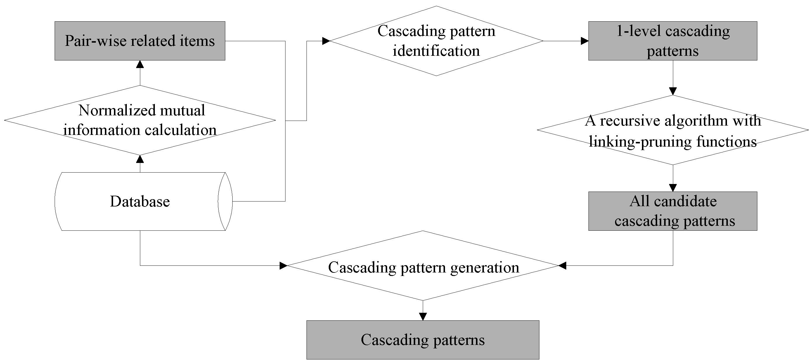
Using the basic concepts and properties described above, the M
3Cap workflow, which involves four key steps, is shown in
Figure 1. The first step calculates the normalized mutual information among items and yields pair-wise related items. The second step generates one-level cascading patterns from pair-wise related items. The third designs recursive linking-pruning functions to generate all candidate cascading patterns. The fourth step retains the meaningful cascading patterns by removing the pseudo patterns from candidates.
3.1. An Algorithm for Producing Pair-Wise Related Items
On the basis of discretization datasets (i.e., a mining transaction table), the database was scanned once to calculate the normalized mutual information between all pairs of items according to Equations (1)–(3), and their normalized mutual information contingency table was constructed.
Table 2 shows its structure. Each element in this table,
I(
Xi,
Xj), indicates that item
Xi provides information about item
Xj, which is represented in the form “
Xi → Xj”.
In general, the mean and standard deviation of the items’ mutual information are used to reveal highly related items [
23]. Here, only the elements within the table fulfilling the following inequality are regarded as pair-wise related items.
where, µ and σ are the mean and standard deviation of the mutual information when
i is not equal to
j, respectively, and λ is a scalar factor. Owing to the asymmetry of the pair-wise related item, “
Xi → Xj”, we define
Xi as an antecedent and
Xj as a consequent.
3.2. One-Level Cascading Patterns with Quantitative Ranks
This step produces all the one-level cascading patterns with quantitative ranks from pair-wise related items. Quantitative ranks represent an item’s variations. In general, not all of the pair-wise related items with quantitative ranks are meaningful. That is to say, only the item’s quantitative ranks with a frequency not less than the evaluation thresholds are retained. Thus, this issue requires three steps. The first step extracts meaningful related items with quantitative ranks by scanning the database once. The second step generates candidate one-level quantitative cascading patterns through the permutation and combination of the meaningful items with quantitative ranks. The third step obtains one-level cascading patterns from candidates by scanning the database using the following criterion, i.e., a frequency not less than the user-specified support and a cascading index not less than the user-specified threshold. The database is scanned once for each candidate one-level quantitative cascading pattern. Thus, all one-level cascading patterns are obtained. Algorithm 1 shows the pseudo-code for this function.
| Algorithm 1. Algorithm for identifying one-level cascading patterns from pair-wise related items. |
| Algorithm name: OneLevelCascadingPatternIdentification. |
| Algorithm description: Identifying all one-level cascading patterns with quantitative ranks from pair-wise related items. |
| Input parameters: Pair-wise related items, denoted as PI, and a quantitative rank, denoted as R. |
| Output parameters: One-level cascading patterns, denoted as 1-CP. |
| 1 | OneLevelCascadingPatternIdentification (PI, R, 1-CP) |
| 2 | FOR ith pair-wise related item in PI, denoted as ith − pi. |
| 3 | Extract its antecedent and consequent, denoted as Xi and Xj, respectively |
4
5
6 | Permute and combine the Xi and Xj with quantitative ranks, i.e., r and l, respectively, where r, l ∈R, then generate candidates of cascading pattern in a form of Xi[r] → Xj[l]. |
| 7 | FOR each Xi[r] → Xj[l] |
8
9 | Scan the database one time, and calculate the supports of Xi and Xj with quantitative ranks through the Equation (4). |
10
11 | IF the following inequalities are true, where τS is the support threshold. |
| 12 | |
13
14 | The Xi and Xj with the quantitative rank r and l are retained, i.e., Xi[r] and Xi[l]. |
| 15 | END IF |
16
17 | Using Equations (4) and (5), calculate its support and cascading index. |
18
19 | IF the following inequalities are true, where τCI is the cascading index threshold. |
| 20 | |
21
22
23 | Link Xi[r] and Xj[l] in a form with Xi[r] → Xj[l], denote it as one-level cascading pattern, i.e., 1-cp, and store it into1-CP. |
| 24 | END IF |
| 25 | END FOR |
| 26 | i = i + 1 |
| 27 | END FOR |
Line 10 to Line 12 are discriminant criteria, which are used to find the meaningful items with a specified quantitative rank (Line 13 to Line 14), similarly, Line 18 to Line 20 are done to generate a new one-level cascading pattern. From Line 7 to Line 25, a pair-wise related item with all quantitative ranks is gone through to generate zero to several one-level cascading patterns, and Line 2 to Line 27 are repeated to deal with all pair-wise related items.
Example 3.
Given pair-wise related items X and Y, X and Z, and Y and Z of the forms “X → Y”, “X → Z”, and “Y → Z” are meaningful, and their quantitative ranks set to 5 from −2 to 2 with a continuous interval. Quantitative datasets are shown in Table 3. The support and cascading index thresholds are set to 30% and 60%, respectively. According to
Table 3, the frequencies of
X[2],
X[1],
X[0],
X[–1], and
X[–2] are 50%, 0%, 10%, 30%, and 10%, respectively, and the frequencies of
Y[2],
Y[1],
Y[0],
Y[–1], and
Y[–2] are 40%, 30%, 20%, 0%, and 10%, respectively, while those of
Z[2],
Z[1],
Z[0],
Z[–1], and
Z[–2] are 0%, 0%, 20%, 30%, and 50%, respectively. According to the support threshold, only
X[2],
X[–1],
Y[2],
Y[1],
Z[–1], and
Z[–2] are meaningful. With the pair-wise related items, “
X →
Y,” and through their permutation and combination, the candidate one-level cascading patterns are “
X[2] →
Y[2]”, “
X[2] →
Y[1]”, “
X[–1] →
Y[2]”, and “
X[–1] →
Y[1]”. After applying the user-specified support and cascading index thresholds, only the one-level cascading pattern, “
X[2] →
Y[2],” which has a support of 30% and a cascading index of 60%, is retained. “
X[2] →
Z[−2] (40%,80%)” and “
Y[2] →
Z[−2] (40%,100%)” are obtained similarly.
3.3. Recursive Algorithm for Generating the Candidates of All Cascading Patterns
This recursive algorithm produces all the candidate (m + 1)-level cascading patterns from the m-level patterns according to the linking and pruning functions, where m is not less than one. In this step, the linking and pruning functions are run recursively without scanning the database until no further candidate cascading patterns are generated.
The linking function generates the candidate (m + 1)-level cascading patterns from the one-level and m-level patterns. The pseudo-code for the linking function is shown in Algorithm 2.
| Algorithm 2. Algorithm of linking m-level cascading patterns to generate (m + 1)-level ones. |
| Algorithm name: Linking Algorithm. |
| Algorithm description: Link m-level cascading patterns (i.e., m-CP) to generate (m + 1)-level cascading patterns (i.e., (m + 1)-CP) according to the Property 1 Information Asymmetry. |
| Input parameters: One-level cascading patterns, 1-CP, and m-level cascading patterns, m-CP. |
| Output parameters: (m + 1)-level cascading patterns, (m + 1)-CP. |
| 1 | LinkingAlgorithm (1-CP, m-CP, (m + 1) - CP) |
| 2 | FOR ith m-level cascading pattern in m-CP, denoted as ith m-cp. |
3
4 | Extract its last item, i.e., Xim + 1[rim + 1], and denote it as PostItem, and the others are organized in order in a form with Xi1[ri1] Xi2[ri2]…Xim[rim], denoted as PreItems. |
| 5 | FOR jth1-level cascading pattern in 1-CP, denoted as ith 1-cp. |
6
7 | Extract its antecedent, i.e., Xj1[rj1], denoted as Pre, and consequent, Xj2[rj2], denoted as Post. |
8
9 | IF Pre is same to PostItem, i.e., the items Xj1 and Xim + 1 are same, and the levels rj1 and rim + 1 are equal. AND not find Xj2 in Xi1[ri1] Xi2[ri2]…Xim[rim]. |
10
11
12 | Link m-cp with appending the item Xj2[rj2] in a form with Xi1[ri1] → Xi2[ri2] → … → Xim[rim] → Xim + 1[rim + 1] → Xj2[rj2], denote it as (m + 1)-cp, and store it into (m + 1)-CP |
| 13 | END IF |
| 14 | j = j + 1 |
| 15 | END FOR |
| 16 | I = I + 1 |
| 17 | END FOR |
Lines 8 and 9 provide the linking discrimination criteria. Linkage is performed if and only if the last item of the m-level cascading pattern is the same as the first item of a one-level cascading pattern (i.e., they have the same single item and the same quantitative level). The m-level cascading pattern does not contain the last item of the one-level cascading pattern (Line 10 to Line 12). From Line 8 to Line 13, zero (the discrimination criterion is false) to one (the discrimination criterion is true) linkage is performed. From Line 5 to Line 15, a loop between one m-level cascading pattern with all of the one-level patterns is executed, and Line 2 to Line17 are repeated to generate all of the (m + 1)-level cascading patterns. The key issue in this function is the linking discrimination.
Example 4. There are one-level cascading patterns “X[2] → Y[2]”, “X[2] → Z[−2]”, and “Y[2] → Z[−2]” (Example 3 results). As the cascading patterns are one-level, the input m-CP is also one-CP (i.e., they have the same cascading patterns). For the first cascading pattern in m-CP, “X[2] → Y[2]”, the function goes through the one-CP sequentially. As the first cascading pattern in one-CP is the same as “X[2] → Y[2]”, no linkage is performed. Regarding the second pattern in one-CP, “X[2] → Z[−2]”, as the last item Y[2] is not the same as the first item X[2], no linkage is performed. Regarding the third in one-CP, “Y[2] → Z[−2]”, as the last item Y[2] is the same as the first item Y[2], one linkage is performed and a new form is generated, “X[2] → Y[2] → Z[−2]”. Similarly, the other cascading patterns in m-CP are analyzed, and there is no linkage. Thus, there is only one two-level cascading pattern generated from the one-level cascading patterns, “X[2] → Y[2] → Z[–2]”.
The pruning function removes the false m-level cascading patterns from the candidate m-level patterns according to Properties 2 and 3. The key issue of this step is to find all (m − 1)-level subpatterns of cascading patterns of an m-level pattern. As long as one subpattern is not an (m − 1)-level cascading pattern, the m-level candidate cascading pattern is removed. Otherwise, the candidate cascading pattern is retained. The pseudo-code for the pruning function is shown as Algorithm 3.
| Algorithm 3. Pruning algorithm to remove the pseudo cascading patterns. |
| Algorithm name: PruningAlgorithm. |
| Algorithm description: Remove the pseudo cascading patterns from the m-level candidates of cascading patterns, denoted as m-CCP, to generate m-level cascading patterns, denoted as m-CP, according to the Property 2. Information Non-Additivities and Property 3. Antimonotonicity. |
| Input parameters: m-level candidates of cascading patterns (i.e., m-CCP) and (m − 1)-level cascading patterns, denoted as (m − 1)-CP. |
| Output parameters: m-level cascading patterns (i.e., m-CP). |
| 1 | PruningAlgorithm (m-CCP, (m − 1)-CP, m-CP) |
| 2 | FOR ith m-level candidate of cascading pattern in m-CCP, denoted as ith m-ccp. |
| 3 | Extract its (m − 1)-level subsets, denoted as (m − 1)-S. |
| 4 | FOR jth(m − 1)-level cascading pattern in (m-1)-S, denoted as jth(m − 1)-s |
| 5 | IF jth(m − 1)-s is not found in (m − 1)-CP |
| 6 | GO TO Line 11 |
| 7 | END IF |
| 8 | J = j + 1 |
| 9 | END FOR |
| 10 | ith m-ccp is retained as a m-level cascading pattern, and stored into m-CP. |
| 11 | ith m-ccp is removed |
| 12 | I = I + 1 |
| 13 | END FOR |
Line 5 is the removal discrimination criterion. As long as one (m − 1)-level subpattern of the candidate m-level pattern is not found among the (m − 1)-level cascading patterns, the candidate m-level cascading pattern is removed (Line 11) and the next candidate m-level cascading pattern is processed (Line 12). If all the (m − 1)-level subsets of the candidate m-level cascading pattern are (m − 1)-level cascading patterns, the candidate m-level cascading pattern is taken as m-level one (Line 10). From Line 4 to Line 9, a loop is executed through all of the (m − 1)-level subsets sequentially to determine the cascading patterns. Line 3 extracts all of the (m − 1)-level subpatterns of an m-level cascading pattern, and Line 2 to Line 13 are repeated to distinguish all of the candidate m-level cascading patterns.
3.4. Generating Cascading Patterns with Evaluation Indicators
This step generates meaningful cascading patterns from candidates according to the minimum thresholds of the evaluation indicators. Generally speaking, the specified thresholds are defined by users according to their research domains. The evaluation indicators of each cascading pattern, including support and cascading index, are calculated by scanning the database once. If the evaluation indicators satisfy the user-specified thresholds, shown in Equation (18), a cascading pattern is meaningful. The support threshold,
σs, means the minimum co-occurrence probability of the
Pattern in the database, while the cascading index,
σCI, means the minimum occurrence probability of each sub-pattern in the database against the
Pattern occurrence. In this step, the key issue is to scan the database and calculate the evaluation indicators.
4. Experiments
This section addresses three case studies for M3Cap using long time series of remote sensing images. The first experiment analyzes the M3Cap’s computational complexity from the viewpoints of database scanning and intensive computing, the second illustrates the feasibility and effectiveness of M3Cap compared with the derived Apriori algorithm, and the third explores the cascading patterns for marine environmental elements in the Pacific Ocean.
These cases was conducted on long-term marine remote sensing images that showed monthly anomalies of sea surface temperature, named SSTA, monthly anomalies of sea surface chlorophyll-
a, CHLA, monthly anomalies of sea surface precipitation, SSPA, and monthly anomalies of sea level anomaly, SLAA. The multivariate ENSO index (MEI) was used to identify ENSO events.
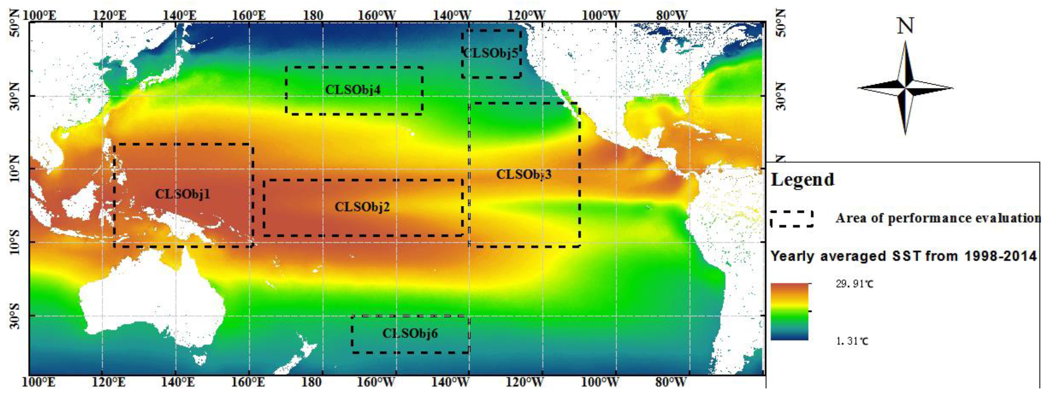
Table 4 summarizes the datasets used. Marine environmental parameters are ranked into five levels for continuous intervals (–2, –1, 0, 1, and 2) that indicate severe negative change, slight negative change, no change, slight positive change, and severe positive change, respectively. As for the MEI index, –2 indicates strong La Niña events, while +2 indicates strong El Niño events [
26]. Monthly image datasets with a spatial resolution of 1° in latitude and longitude from January 1998 to December 2014 for six different regions in the Pacific Ocean, which are denoted as CLSObj1, CLSObj2, CLSObj3, CLSObj4, CLSObj5, and CLSObj6 in
Figure 2, are used to test the algorithms. Each region consists of a series of raster lattices, each containing four parameters, SSTA, SSPA, SLAA, and CHLA, with an ENSO index. The experimental hardware environment includes an Intel core i7 CPU at 2.80 GHz, a 500 GB hard disk, and 4.0 GB of memory.
4.1. Computational Complexity
The computational complexity of M3Cap is classified into two categories—the number of database scans and intensive computing.
Within the M3Cap process, scanning a database involves three stages. The first stage builds the mutual information contingency table by scanning the database once. The second stage identifies the one-level cascading patterns from pair-wise related items with quantitative ranks. For each pair-wise related item with each quantitative rank, there is one database scan. For the given quantitative rank, R, and the total number of items, M, according to the function, OneLevelCascadingPatternIdentification, the number of database scans is (R × M) × (R × (M − 1)) (i.e., R2 × ) and the computational complexity of identifying the one-level cascading patterns is O(R2 × M2). For the third stage, M3Cap uses Equation (15) to find a meaningful cascading pattern for each candidate pattern by scanning the database once. Theoretically, there are R2 × + R3 × + … + RM × M! (i.e., O(R2 × + R3 × + … + RM × M!)) candidate cascading patterns; hence, the computational complexity of finding a meaningful cascading pattern is o(R2 × M2) + o(R3 × M3) + … + o(RM × MM). However, in reality, the candidate cascading patterns are reduced substantially in accordance with the information threshold and Properties 2 and 3, which are substantially less than R2 × + R3 × + … + RM × M!.
M3Cap involves two stages of intensive computing. One stage obtains the pair-wise related items from a mutual information contingency table. There are M × (M − 1) discriminations to determine the related items according to the information threshold; hence, the computational complexity is O(M2). The other stage generates candidate cascading patterns using a recursive linking and pruning algorithm. In the linking phase, according to Linking Algorithm, the (m + 1)-level cascading patterns are generated by linking m-level and one-level patterns, and the number of linkings is R2 × M2 × Rm × ; thus, the linking complexity is o(R2 × M2 × Rm × ) = o(R2 + m × M2 + m). In the pruning phase, for each candidate (m + 1)-level cascading pattern, there are (m + 2) subpatterns of an m-level cascading pattern. Each subset needs a calculation to determine whether the (m + 1)-level cascading pattern is to be removed. The number of discriminations is R2 × M2 × Rm × × (m + 2); therefore, the pruning complexity is o(m × R2 + m × M2 + m).
4.2. Factors Affecting the Performance of M3Cap
Given a quantitative rank, three factors affect the performance of M3Cap. They are information threshold, evaluation threshold, and database size (i.e., the number of database fields (the derived items)) and records. The information threshold determines how many items are pair-wise related and influences the database base scanning times. The evaluation thresholds are determined by database scanning the number of meaningful cascading patterns from among the candidates. The database fields determine the database scanning time, and the database records determine the computation time for database scanning.
4.2.1. Information Threshold
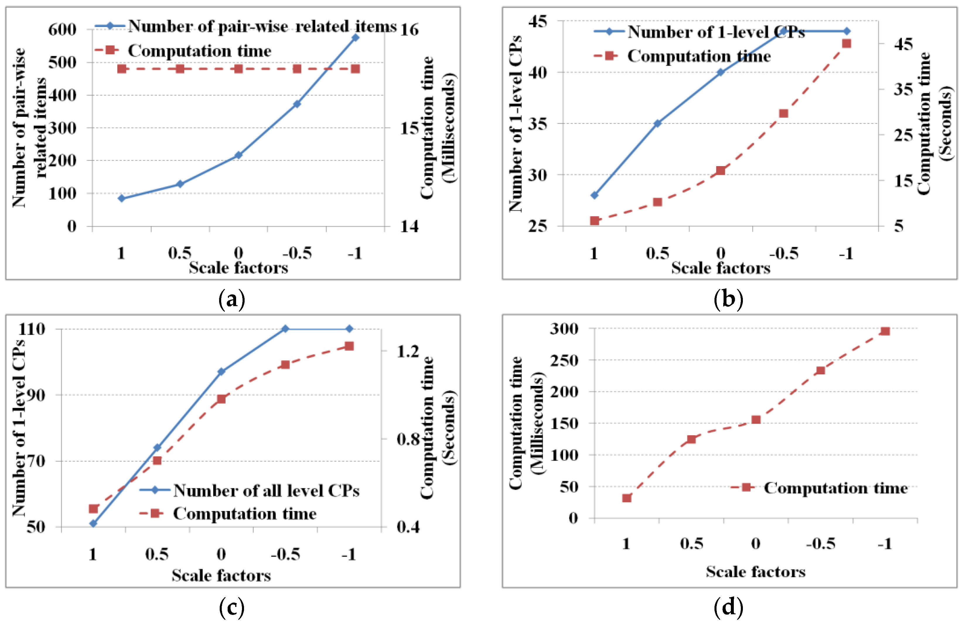
The mutual information threshold determines the initial pair-wise related items and then obtains cascading patterns. According to Equation (14), the threshold is calculated through the 1.0 mean plus λ standard deviation of the items’ mutual information. In this experiment, the support and cascading index thresholds are set to 5% and 75%, respectively, and λ is 1.0, 0.5, 0.0, −0.5, and −1.0.
Figure 3 shows the performance under mutual information thresholds with different λ values.
Given the support and cascading index thresholds, the smaller the mutual information threshold, the more the pair-wise related items, and then the more one-level and total cascading patterns. Regarding the computation time, to determine which items are related from the mutual information contingency table, the number of discriminations to obtain the related items is fixed (e.g., 25 × 24). Thus the computation time is fixed (i.e., 15.6 ms) whether λ is large or small (
Figure 3a). The computation time to find the one-level and total cascading patterns is determined by the number of database scans (i.e., the number of pair-wise related items and candidate cascading patterns). Hence, the smaller the mutual information threshold, the greater the computation time for finding one-level and total cascading patterns (
Figure 3b,c), and vice versa. Similarly, the number of candidate cascading patterns determines the number of linkings and prunings; hence, the smaller the mutual information threshold, the greater the computation time of linking and pruning (
Figure 3d). If the database is not scanned, then this computation time is reduced substantially.
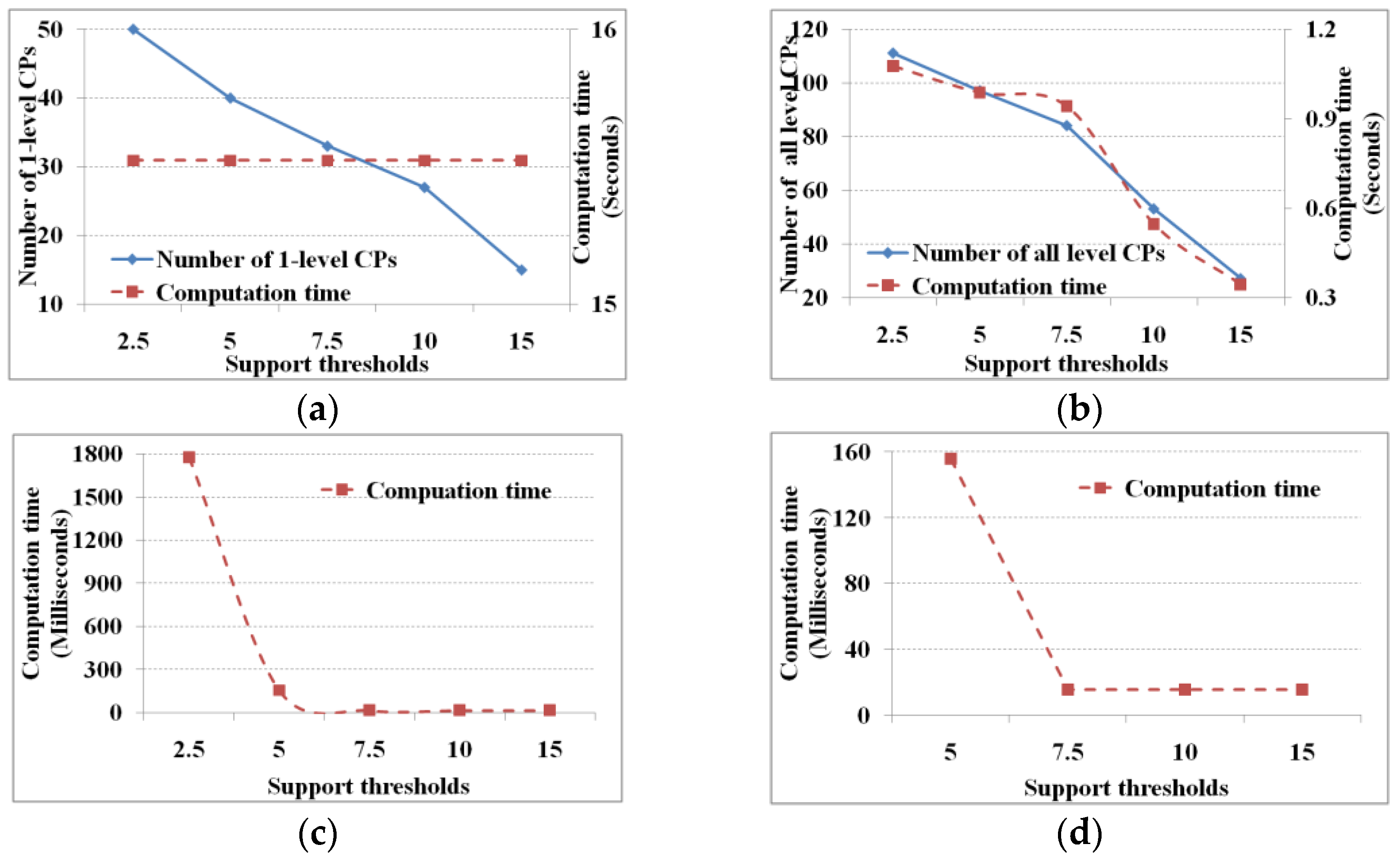
4.2.2. Evaluation Thresholds
The evaluation thresholds include a support and a cascading index threshold, which are largely defined according to user requirements and domain. M
3Cap involves two stages in which it uses the evaluation thresholds to find cascading patterns. One stage identifies one-level cascading patterns from pair-wise related items, while the other stage generates meaningful cascading patterns from all the candidates. In this experiment, 25 items within six regions with 204 records are used to test the algorithm; the scale factor of mutual information threshold is set to the mean value (i.e.,
) and the support and cascading index thresholds are set to 5% and 75%, respectively.
Figure 4 and
Figure 5 show the performance under different support and cascading index thresholds, respectively.
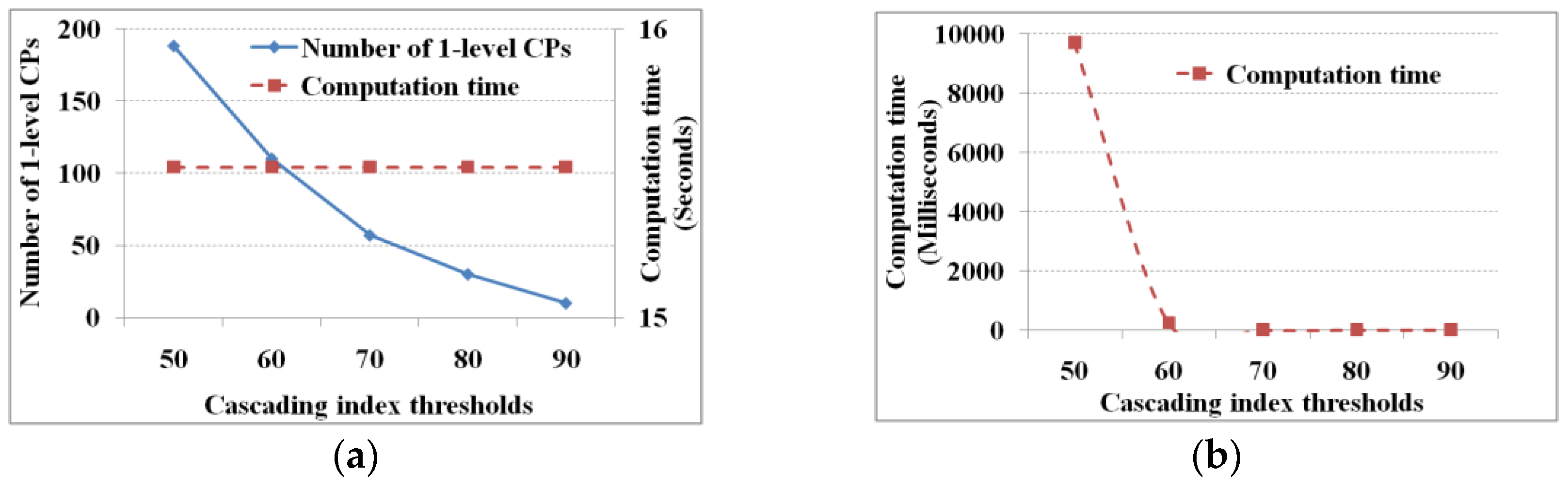
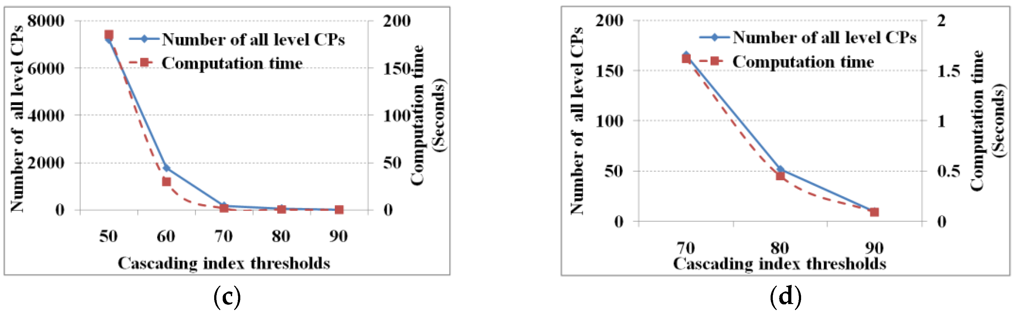
From
Figure 4 and
Figure 5, we know that the lower the evaluation thresholds, the greater are the number of cascading patterns, and vice versa, and the computation time of finding all cascading patterns decreases with increasing thresholds. However, the computation time to find one-level cascading patterns is fixed (i.e., 15.6 s) whether the thresholds are high or low. Given a mutual information threshold, we will get a fixed number of pair-wise related items and database scanningtimes; hence, the computation time of finding the one-level cascading patterns is fixed. As for the computation time of the linking and pruning function, theoretically it is expected to decrease along with increasing evaluation thresholds. However, when the evaluation thresholds reach a specific value (support and cascading index thresholds of 7.5% and 70%, respectively) the computation time does not change. When the threshold reaches the specific value, the linking and pruning times are too small to show changes in computation time. That is to say, when the threshold reaches the specified value, the computation time is shown as a computational unit (i.e., 15.6 ms on our test computer).
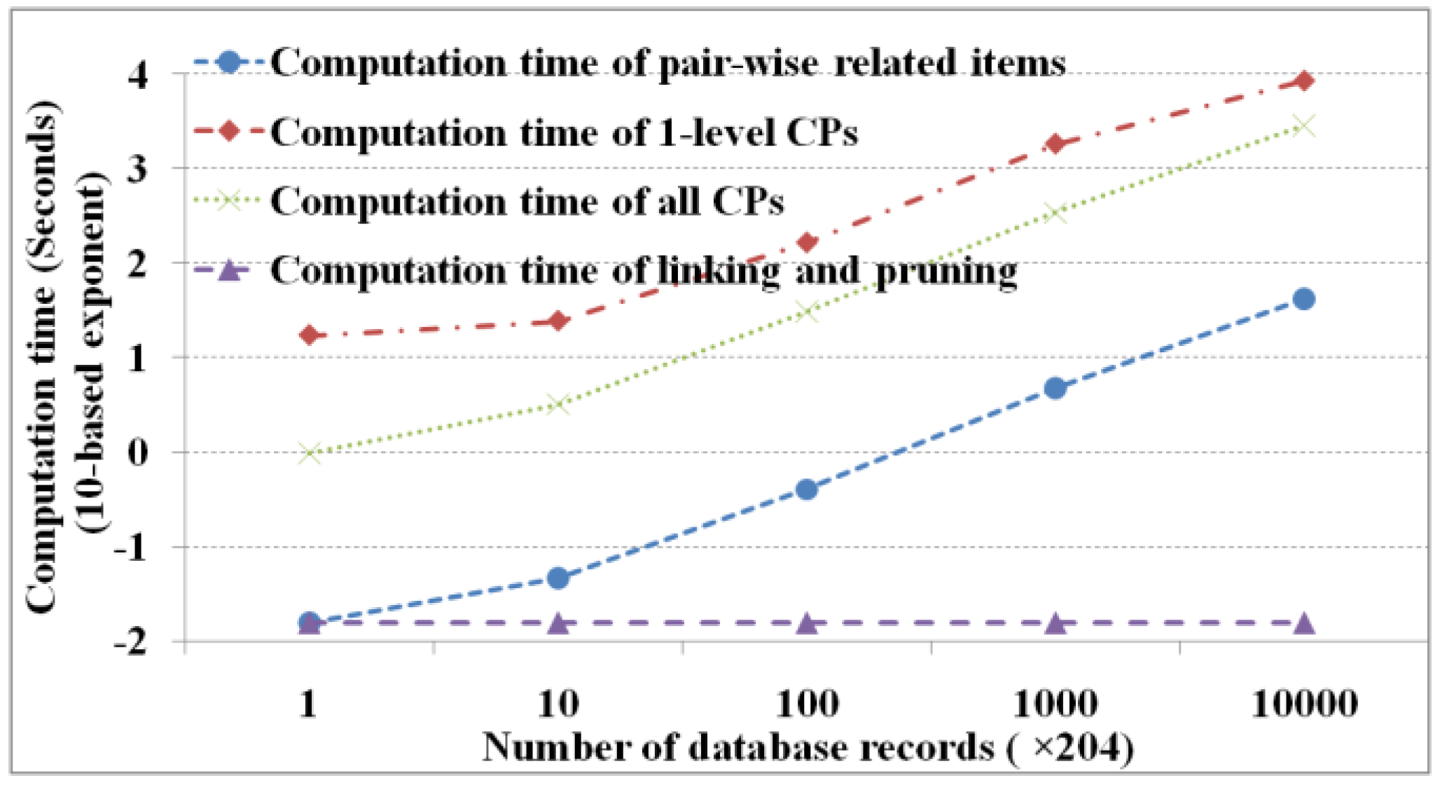
4.2.3. Database Size
The database size consists of the record and field number. The former represents the number of samples, and the latter represents the derived items. In this experiment, the support and cascading index thresholds are set to 5% and 60%, respectively, and
is set to zero. Regarding the database records, 1, 10, 100, 1000, and 10,000 copies of 204 records (January 1998 to December 2014) with 25 items (six regions with four parameters and ENSO index) from remote sensing images are produced. As we are mining with duplications, we get similar results with 216 pair-wise related items, 40 one-level cascading patterns, and 97 total cascading patterns.
Figure 6 shows the performance of M
3Cap under different record numbers (i.e., 204 × 10
0, 204 × 10
1, 204 × 10
2, 204 × 10
3, and 204 × 10
4, respectively).
Figure 6 shows that maximum computation time occurs in finding the one-level cascading patterns then in finding all cascading patterns and pair-wise related items in order and finally in linking and pruning. The computation time is dominated primarily by the number of database scans, which is determined by the number of database records. In this experiment, there are 216 × 25 database scans to find one-level cascading patterns, 105 to find all cascading patterns, and one to construct a mutual information contingency table and obtain the pair-wise related items. Apart from the effects of the database records, the computation time of linking and pruning is fixed irrespective of a database record size. In addition, we know that except for linking and pruning, the computation time increases exponentially with an increase in the number of database records.
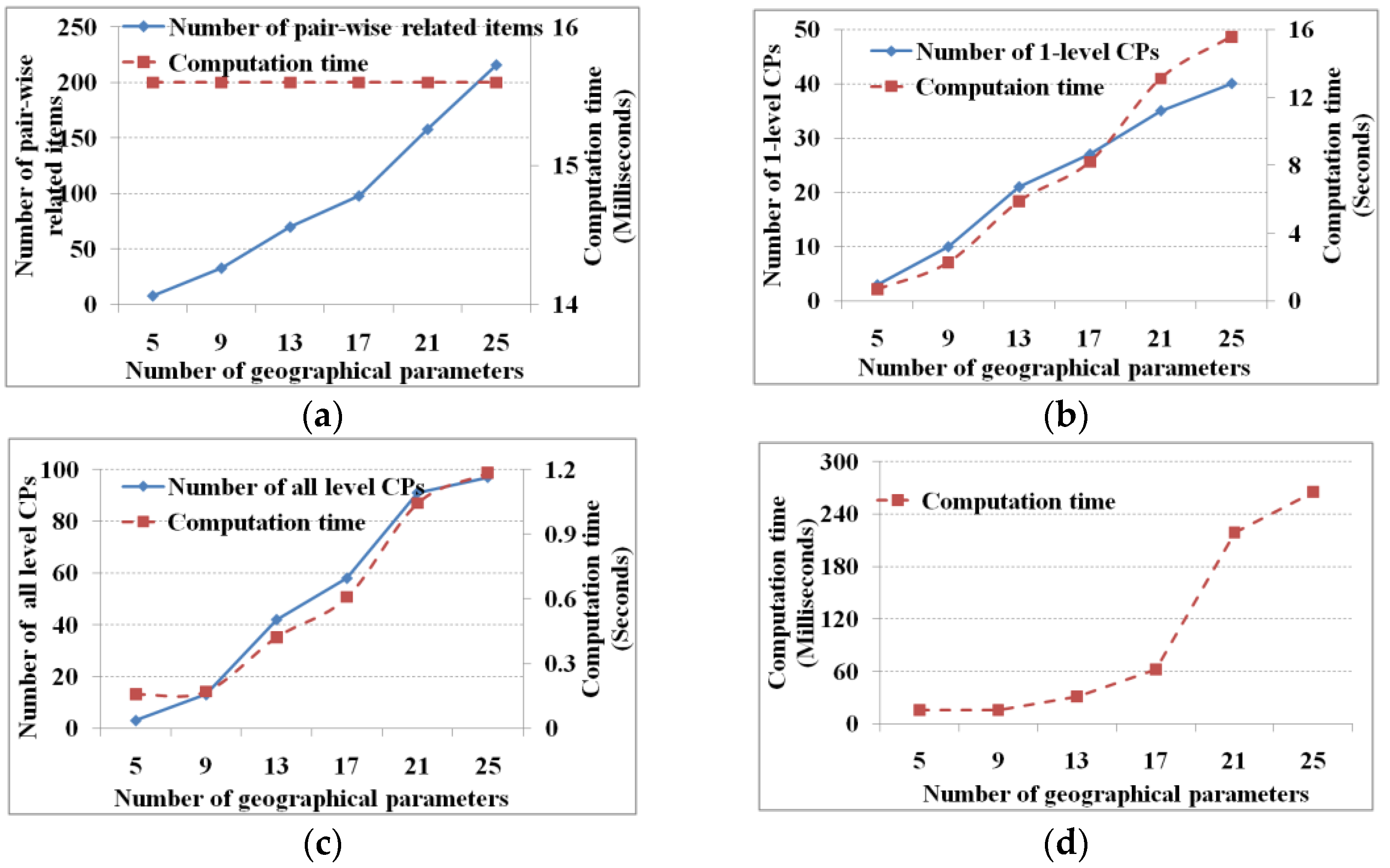
To test the field number on the performance of M
3Cap, we combine the four marine parameters within each region (i.e., CLSObj1 to ClSObj6 with ENSO index, as shown in
Figure 2). Thus, 5, 9, 13, 17, 21, and 25 fields are used (e.g., the five fields are the four marine parameters in the CLSObj1 region with the ENSO index, the nine fields are the four marine parameters in the CLSObj1 and CLSObj2 regions, respectively, with ENSO index, and so on). In this experiment, the support and cascading index thresholds are set to 5% and 75%, respectively, and
is set to zero. The results are shown in
Figure 7.
Along with the increase in the number of items, we spend more time to obtain the further numbers of one-level and all-level cascading patterns (
Figure 7b,c) and to further link candidate cascading patterns and remove pseudo patterns (
Figure 7d). Although we obtain more pair-wise related items, the computation time is almost fixed (
Figure 7a). The reason lies in that the computation time focuses on discrimination times, which changes from 5 × 4, 9 × 8, 13 × 12, 17 × 16, 21 × 20 to 25 × 24. Comparative to the computational abilities, the computation time for discriminating pair-wise related items gives no significant change.
4.3. Comparisions with the Quantative GSP
We use the generalized sequence pattern, GSP [
12], as the baseline for comparison on the efficiency of the M
3Cap algorithm. The three core steps of GSP are (1) finding the frequent 1-items to generate one-level sequence patterns; (2) linking and pruning to generate candidate patterns; and (3) counting candidates to find meaningful sequence patterns. For dealing with the quantitative patterns, the quantitative GSP is derived from the core idea of GSP, and in order to make a fair comparison, the quantitative GSP uses the same discretization strategy, the support and cascading index thresholds as the M
3Cap.
In this experiment, 25 items within six regions with 204 records are used to test the algorithms, the scale factor of mutual information threshold is set to the mean value (i.e.,
), and the support and cascading index thresholds are set to 5% and 75%, respectively. For a clear comparison, both GSP and M
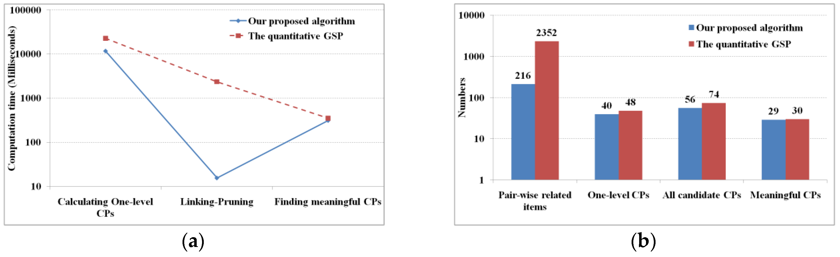
3Cap are divided into three mining phases (i.e., a calculating of one-level cascading patterns, a recursive of linking and pruning, and a finding of meaningful cascading patterns).
Figure 8 shows their computation time and results, and
Table 5 shows a comparison of parts of the mined meaningful cascading patterns (only the cascading patterns with a support not less than 15.00%).
In the quantitative GSP algorithm, a calculating of one-level CPs includes the steps of finding frequent 1-items and of generating two dimensional association patterns (i.e., one-level cascading patterns) while in M
3Cap, this includes the steps of identifying pair-wise related items and of generating one-level cascading patterns. In this step, the M
3Cap is two times faster than GSP, i.e., the former takes 11.6 s, while the latter dose 22.9 s (
Figure 8a). The reason lies in that M
3Cap scans database one time to calculate the items’ mutual information, and then generates the pair-wise related items, while GSP scans the database once for each item to identify it frequent or not, and then generates the pair-wise related items. From pair-wise related items to one-level cascading patterns, both GSP and M
3Cap scan the database once for each pair-wise related item, however, the former deals with 2352 pieces of pair-wise related items, while the latter does 216 pieces. In the recursive of the linking and pruning phase, both GSP and M
3Cap generate all the candidates of cascading patterns. The former will scan database once for each candidate cascading pattern, while M
3Capwill not, therefore, M
3Cap computes all candidates of cascading patterns up to two orders of magnitude faster than GSP. In the final step, M
3Cap and GSP have the similar processing method of finding meaningful cascading patterns by scanning the database once for each candidate, thus, their computing efficiencies have no significant differences.
Table 5 shows that the mined results from M
3Cap and GSP are the same, except that GSP finds an additional patterns, “CHLA-CLSObj1[-1] → SSTA-CLSObj1[2], 15.00%, 93.10%”. The reason lies in the selection of the mutual information threshold. The standard mutual information from CHLA-CLSObj1 to SSTA-CLSObj1 is 0.100, while the mean standard mutual information for all the items, the information threshold, is 0.104. That is to say, the candidate “CHLA-CLSObj1 → SSTA-CLSObj1” is missed when the pair-wise related items are found at the first step, so the pattern is not found by the M
3Cap algorithm.
4.4. Marine Cascading Patterns in the Pacific Ocean
Supposed the cascading patterns in
Table 5 are meaningful (fitting to the minimum support and cascading index thresholds), some well-known interrelationships within the Pacific Ocean are obtained: the variation of SSTA, SLAA, or co-variations between SSTA and SLAA mostly are dominated by ENSO, Pacific Decadal Oscillation, and Pacific-North American patterns, thus, SSTA and SLAA are more interrelated than other marine environmental parameters (No.2 to No.12) [
33]. When La Niña events occur, the westward Rossby reaches the central Pacific Ocean, which pushes the warm pool at the surface toward the west. At the same time, the North Pacific Current flows eastward through the middle of the northern subtropical Pacific Ocean, resulting in mean SST increases. So, SSTA in regions CLSObj2, CLSObj3 and CLSObj4 is a response to a La Niña event (No.13 to No.15) [
2]. In addition, we can also discern much more quantitative information among marine environmental parameters, and identify lesser-known patterns from multiple marine environmental parameters, such as in No.16, meaning that an abnormal decrease of SSTA in region CLSObj4 may be a response to a La Niña event. From two- to more- level cascading patterns (No.17 to No.30) we also find some relationships in order in different regions. Such patterns may be new to Earth scientists.
5. Discussion and Conclusions
This paper proposes a novel algorithm—M3Cap—for mining cascading patterns and tests the algorithm using remote sensing image datasets. By delving into the mutual information to extract the initial pair-wise related items and using a recursive linking and pruning function without database scanning, M3Cap reduces the number of database scans substantially and improves computational efficiency.
Although our proposed M
3Cap has a workflow similar to the previously proposed MIQarma [
24], the two approaches are essentially different. M
3Cap focuses on cascading characteristics, while MIQarma deals with association characteristics; hence, they differ in the key issue of linking and pruning. With no database scanning during the linking and pruning, the efficiency of M
3Cap increases. In addition, the core idea of M
3Cap is based on quantitative GSP [
12], but the two algorithms differ in initial pair-wise related item (frequent two-item) extraction, linking and pruning, and evaluation indicators.
Analysis of computational complexity shows that M3Cap involves four stages—extraction of pair-wise related items, recursive linking and pruning to obtain all of the candidate cascading patterns, extraction of one-level cascading patterns, and generation of meaningful cascading patterns. The first two stages involve intensive computing and are dependent on the number of derived items and on linking and pruning. The other two are dependent on the number of database scans and the time for scanning the database once. Theoretically, the second stage involves the most complex intensive computing; however, with no database scanning, its computational complexity is simplest.
Regarding database scanning times, the mutual information threshold is one of the most important factors. Given the number of derived items, a smaller mutual information threshold will result in more initial related pair-wise items and more database scans, and vice versa. Thus, the key issue is to determine the mutual information threshold. M
3Cap combines the mean and standard deviation of the items’ mutual information, which is commonly used to reveal highly related items [
21]. Moreover, many experiments show that when a mutual information threshold is between a value of the mean subtracting one standard deviation and a value of the mean adding one standard deviation (i.e., a scalar factor is between −1 and 1), we will obtain approximate cascading patterns as typical mining algorithms. In addition, the evaluation thresholds, a support threshold and a cascading index, affect the number of database scans. The smaller the evaluation indicators, the more the one-level cascading patterns, then the more other-level patterns, then the more times of database scanning, and vice versa. In this paper, the evaluation thresholds are defined according to users’ requirements and domain. Experiments with remote sensing image datasets showed that the computation time of database scanning once is mostly dominated by the number of database records. A greater number of database records results in a greater computation time for database scanning. However, the linking and pruning computation time with different thresholds, shown in
Figure 4c and
Figure 5b, contradict the theoretical analysis. Theoretically, as evaluation thresholds increase, the candidate cascading patterns decrease and the linking and pruning time decreases along with its computation time. However, when the support threshold and cascading index reach 7.5% and 70%, respectively, their computation times do not decrease because the linking and pruning time is too short to show changes in the computation time. Similarly, given a mutual information threshold, the more the derived items, the more the discrimination criterion is applied to obtain pair-wise related items and the more computation time is then required. However, the computation time does not change, as
Figure 7a shows. The number of derived items changes from 5 to 25, and the number of applications of the discrimination criterion changes from 5 × 4 to 25 × 24 correspondingly. The limited discrimination criterion times are not sufficient to be able to show changes in computation time.
In summary, faced with the challenge of finding cascading characteristics, we proposed the M
3Cap method and tested it using real remote sensing image datasets. The main conclusions of our study are the following:
We designed the M3Cap workflow and discussed M3Cap computational complexities by absorbing mutual information. According to the two categories of complexity—intensive computing and database scans—four key steps were presented.
Two stages dominate intensive computing, obtaining pair-wise related items from a mutual information contingency table according to the discrimination criterion, which is dominated by the number of derived items, and generating all of the candidate cascading patterns from one-level patterns by recursive linking and pruning. Having no database scanning substantially reduces computational complexity.
The mutual information and evaluation thresholds and the database size are the main factors affecting the number of database scans. The mutual information threshold mainly dominates the initial pair-wise related items and affects the number of candidate cascading patterns indirectly. The evaluation thresholds dominate the time of finding the meaningful cascading patterns. The number of database fields (i.e., the number of derived items) also affects the initial pair-wise related items, then the one-level and all cascading patterns, and the number of database records dominates the time of database scanning once.
Experiments with real remote sensing image datasets covering the Pacific Ocean were conducted to demonstrate the feasibility and efficiency of M3Cap.


