

Mapping VHR Water Depth, Seabed and Land Cover Using Google Earth Data

Abstract
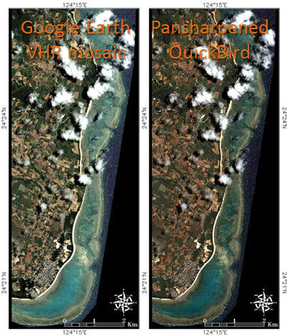
1. Introduction
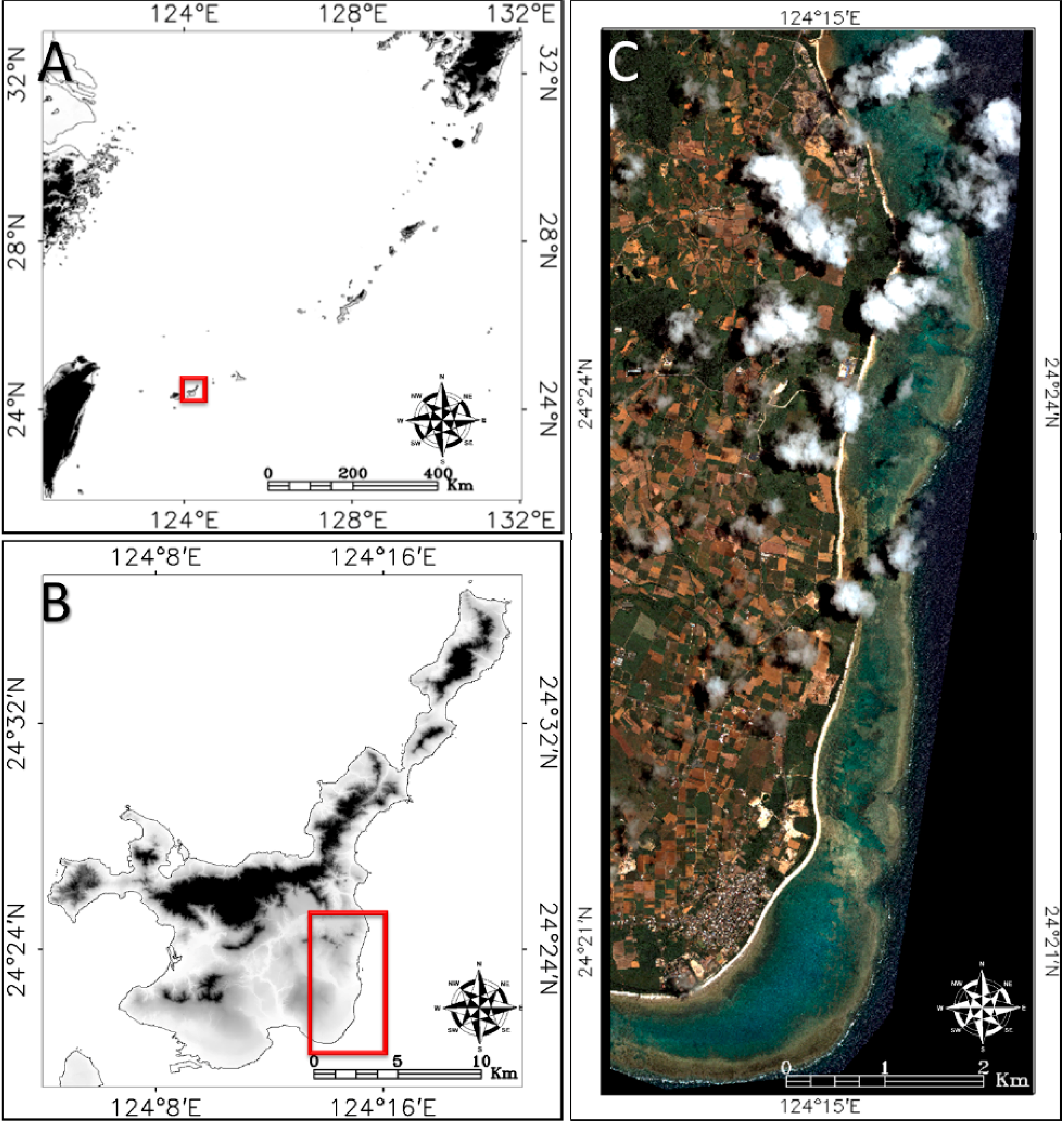
2. Materials and Methods
2.1. Study Site
2.2. Remotely Sensed Datasets
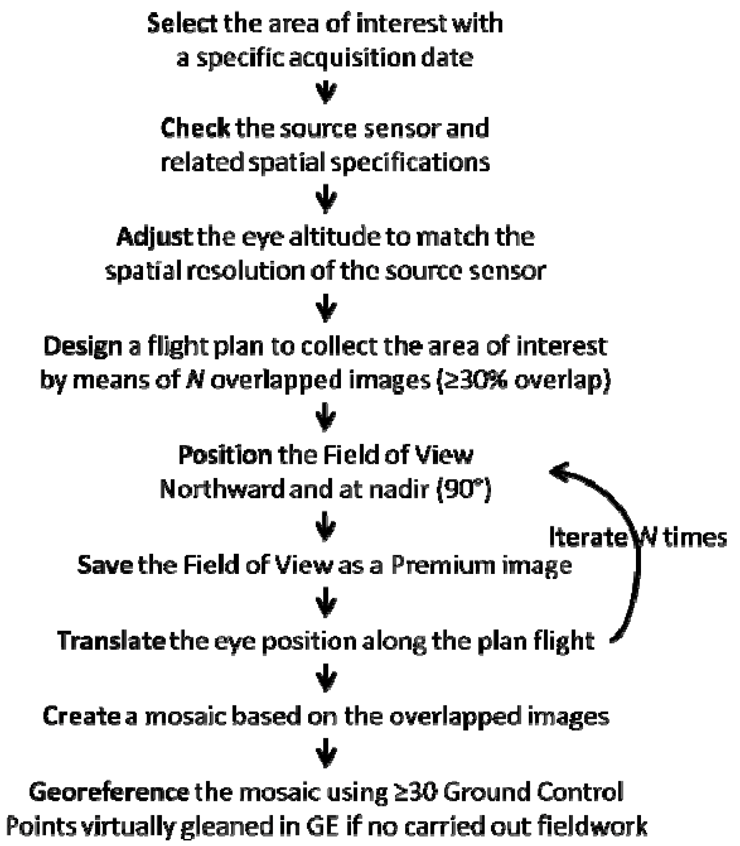
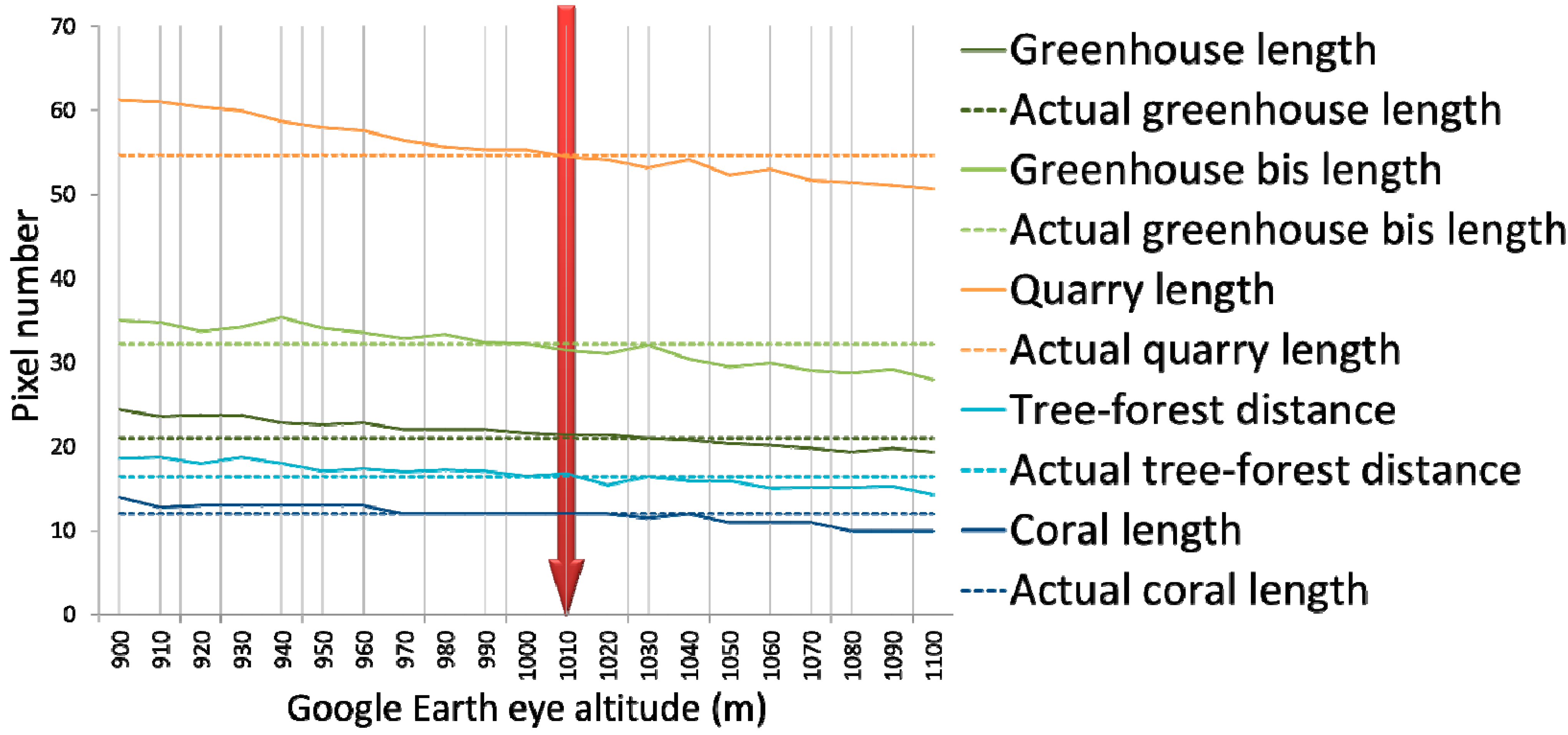
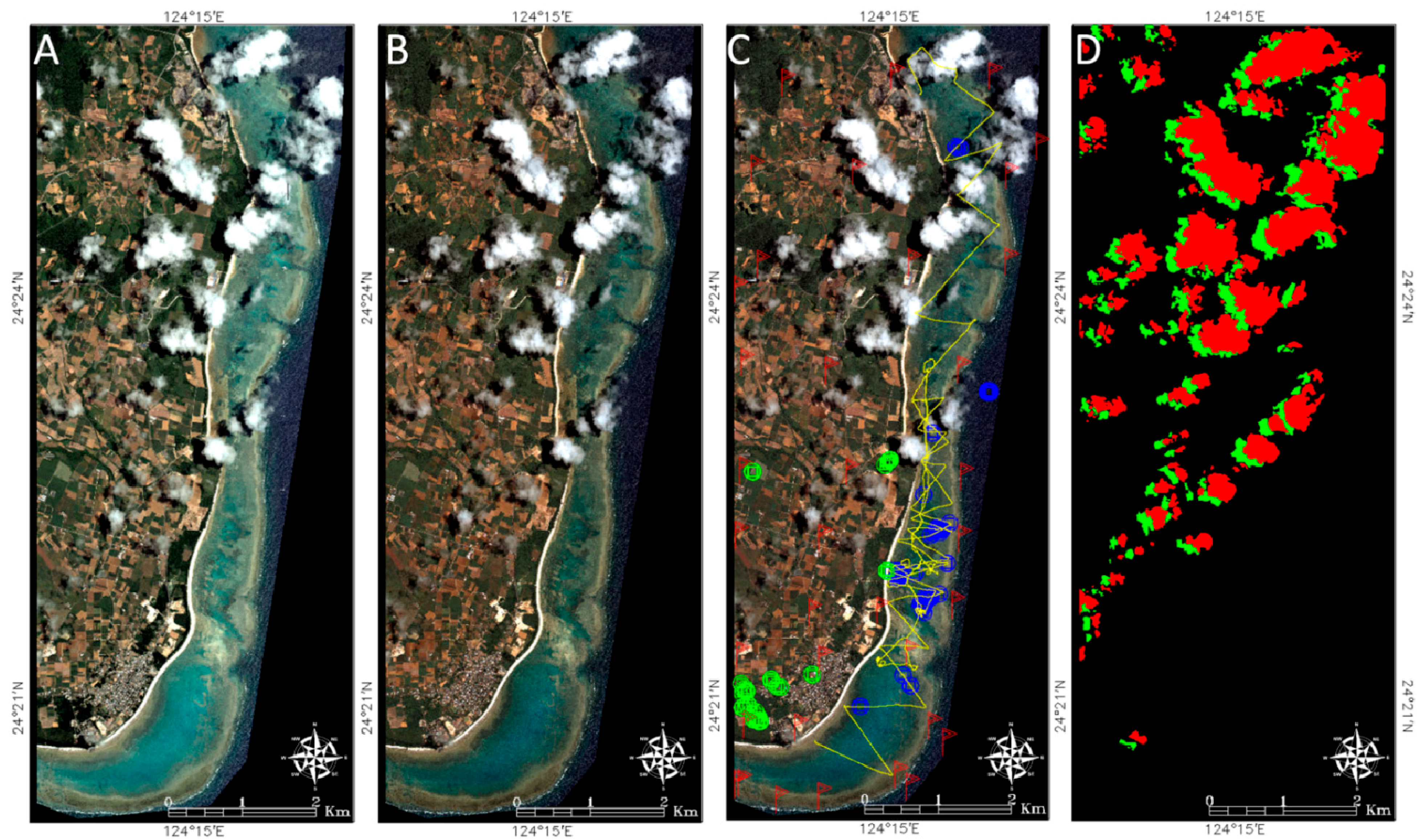
2.3. Coastal Water Depth and Cover Types
2.3.1. Bathymetry and Topography
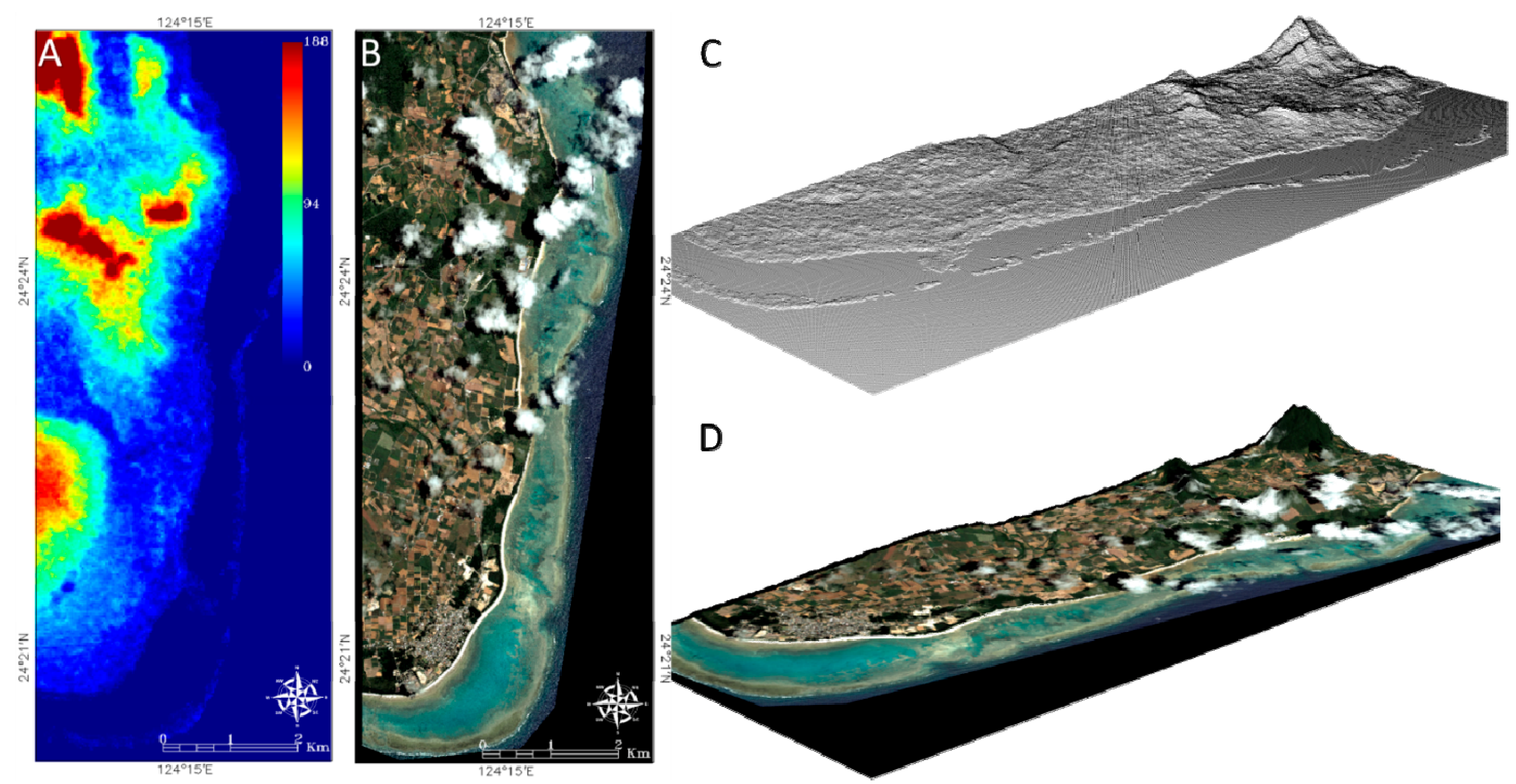
2.3.2. Coastal Cover Types

| Realm | Cover Type | Description |
|---|---|---|
| Marine | Abenthic | Optical deep water |
| Mud | Terrigeneous and coralligeneous clastic sediment below 0.0625 mm grain size | |
| Fine sand | Coralligeneous clastic sediment ranging from 0.0625 to 0.25 mm grain size | |
| Sand | Coralligeneous clastic sediment ranging from 0. 25 to 0.5 mm grain size | |
| Coarse sand | Coralligeneous clastic sediment ranging from 0.5 to 2 mm grain size | |
| Pebble | Coralligeneous clastic sediment ranging from 2 to 64 mm grain size | |
| Cobble | Coralligeneous clastic sediment ranging from 64 to 256 mm grain size | |
| Boulder | Coralligeneous clastic sediment ranging above 256 mm grain size | |
| Blue algae | Cyanobacteria communities eroding consolidated coralligeneous sediment | |
| Brown algae | Tufts or carpets of macroalgae dominated by Turbinaria spp. and Padinae spp. | |
| Calcareous algae | Encrusting algae communities (e.g., coralline) eroding consolidated coralligeneous sediment | |
| Seagrass | Meadows of aquatic phanerogam composed of Cymodocea sp., Halodule sp., Halophila sp., Zostera japonica | |
| Hard coral bommie | Pseudo-spherical massive coral colony dominated by hexacorallian Porites spp. | |
| Hard coral thicket | Field of thicket coral colony dominated by hexacorallian Acropora spp. | |
| Blue coral | Pseudo-spherical massive coral colony dominated by octocorallian Heliopora coerulea | |
| Terrestrial | River | Elongated inland water body |
| Wet sand | Intertidal coralligeneous clastic sediment ranging from 0.0625 to 2 mm grain size | |
| Dry sand | Supratidal coralligeneous clastic sediment ranging from 0.0625 to 2 mm grain size | |
| Soil | Various bare substrata devoid of vegetation (if any, very sparse) | |
| Grass | Natural and mowed herbaceous (≤0.5 m) poaceae communities | |
| Crop field | Cultivated herbaceous vegetables and fruits | |
| Sugar cane field | Cultivated shrub poaceae (≥0.5 and ≤6 m) | |
| Mangrove forest | Natural mix of shrubs and trees (≥6 m) rhizophoraceae | |
| Dark forest | Natural mix of tree aquifoliaceae dominated by Ardisia quinquegona | |
| Road | Anthropogenic infrastructure characterized by asphalt-covered curve lines | |
| Roof | Anthropogenic infrastructure made of ceramic or metallic tiles |
2.3.3. Classification of Coastal Covers and Accuracy Assessment
3. Results
3.1. Comparison of the Water Depth Retrieval
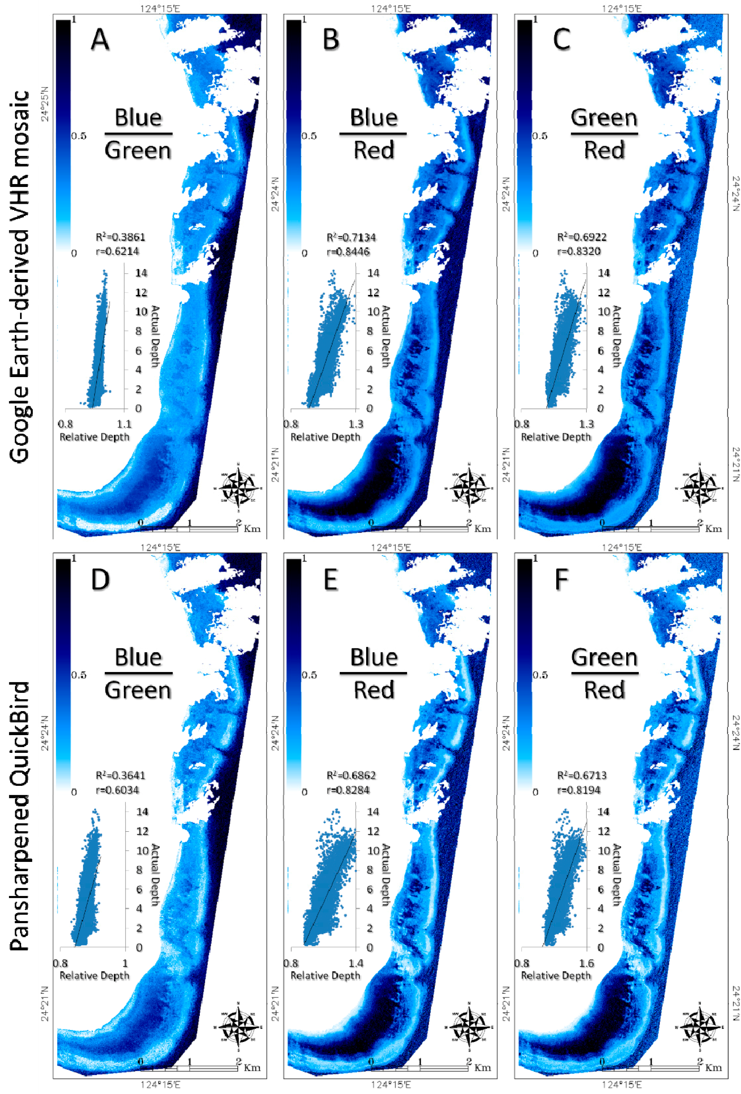
| Google Earth | QuickBird | ||||||
|---|---|---|---|---|---|---|---|
| Blue/Green | Blue/Red | Green/Red | Blue/Green | Blue/Red | Green/Red | ||
| Google Earth | Blue/Green | X | 69.74 | 65.10 | 4.82 | NC | NC |
| Blue/Red | 69.74 | X | 4.92 | NC | 6.29 | NC | |
| Green/Red | 65.10 | 4.92 | X | NC | NC | 4.76 | |
| QuickBird | Blue/Green | 4.82 | NC | NC | X | 68.38 | 65.18 |
| Blue/Red | NC | 6.29 | NC | 68.38 | X | 3.38 | |
| Green/Red | NC | NC | 4.76 | 65.18 | 3.38 | X | |
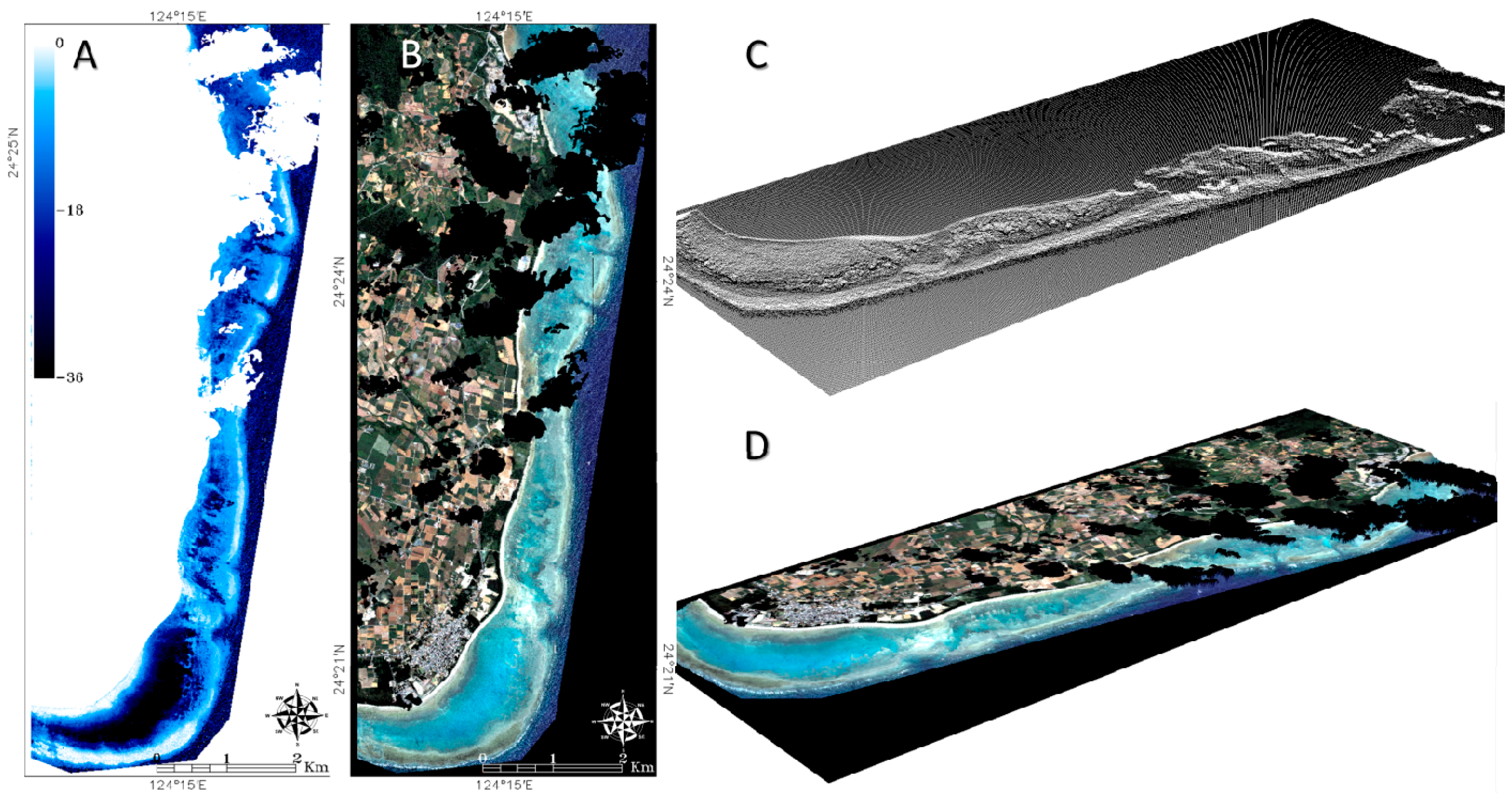
3.2. Comparison of the Seabed Cover Mapping
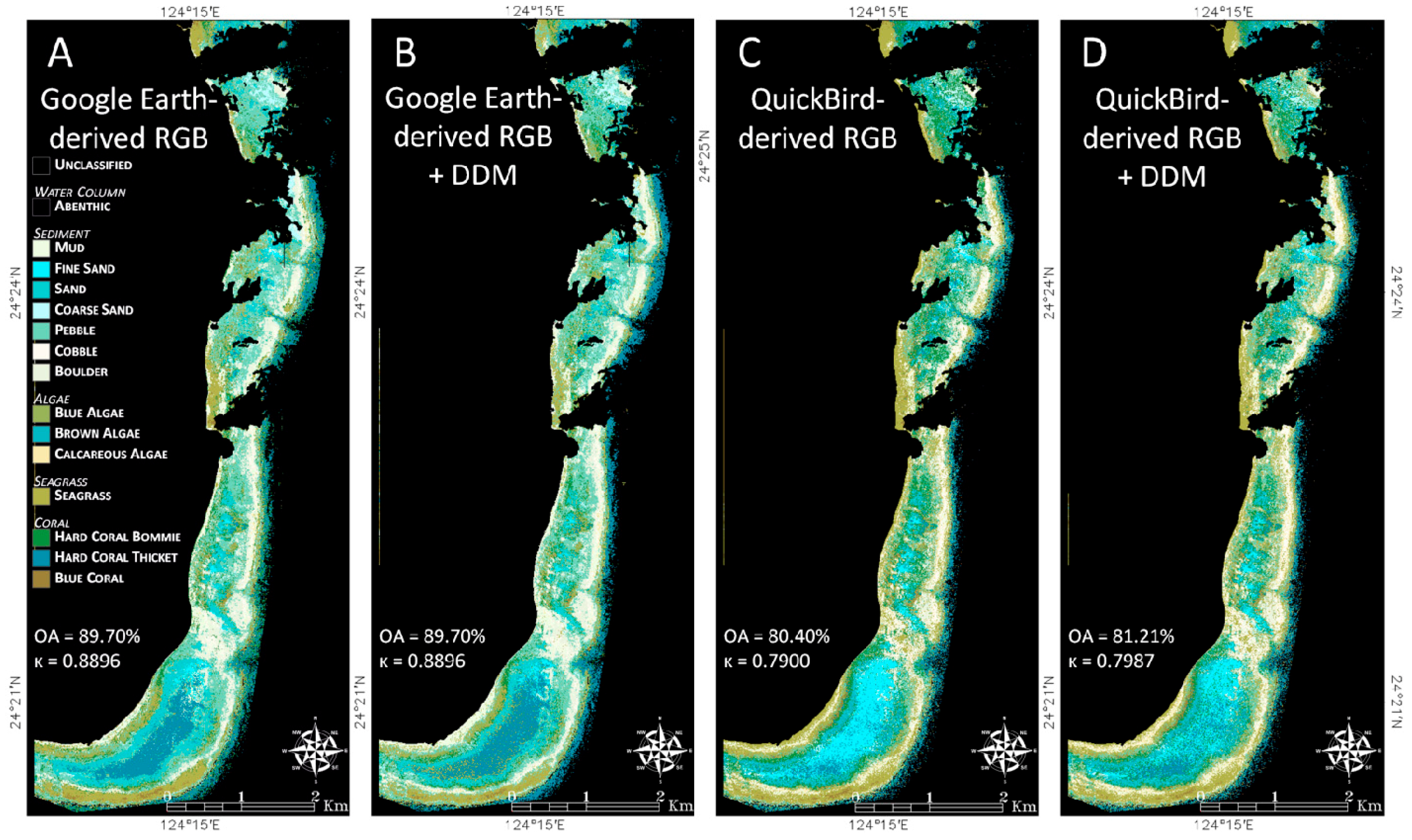
| Google Earth | QuickBird | |||||||
|---|---|---|---|---|---|---|---|---|
| RGB | RGB + DDM | RGB | RGB + DDM | |||||
| PA | UA | PA | UA | PA | UA | PA | UA | |
| Abenthic | 100 | 100 | 100 | 100 | 100 | 100 | 100 | 100 |
| Mud | 90.91 | 100 | 90.91 | 83.33 | 75.76 | 92.59 | 84.85 | 87.5 |
| Fine sand | 100 | 100 | 96.97 | 100 | 100 | 100 | 96.97 | 100 |
| Sand | 100 | 100 | 96.97 | 96.97 | 100 | 97.06 | 96.97 | 94.12 |
| Coarse sand | 100 | 100 | 100 | 94.29 | 100 | 100 | 100 | 91.67 |
| Pebble | 100 | 100 | 75.76 | 60.98 | 100 | 97.06 | 84.85 | 70 |
| Cobble | 100 | 89.19 | 84.85 | 90.32 | 90.91 | 83.33 | 84.85 | 90.32 |
| Boulder | 90.91 | 100 | 100 | 94.29 | 96.97 | 94.12 | 96.97 | 94.12 |
| Blue algae | 100 | 97.06 | 75.76 | 65.79 | 100 | 86.84 | 75.76 | 60.98 |
| Brown algae | 100 | 100 | 96.97 | 96.97 | 96.97 | 100 | 90.91 | 93.75 |
| Calcareous algae | 100 | 94.29 | 72.73 | 77.42 | 96.97 | 91.43 | 78.79 | 74.29 |
| Seagrass | 57.58 | 61.29 | 21.21 | 58.33 | 72.73 | 66.67 | 21.21 | 70 |
| Hard coral bommie | 63.64 | 70 | 54.55 | 66.67 | 81.82 | 77.14 | 60.61 | 68.97 |
| Hard coral thicket | 66.67 | 68.75 | 78.79 | 61.9 | 63.64 | 84 | 78.79 | 68.42 |
| Blue coral | 75.76 | 65.79 | 60.61 | 55.56 | 69.7 | 76.67 | 66.67 | 57.89 |
3.3. Comparison of the Land Cover Mapping
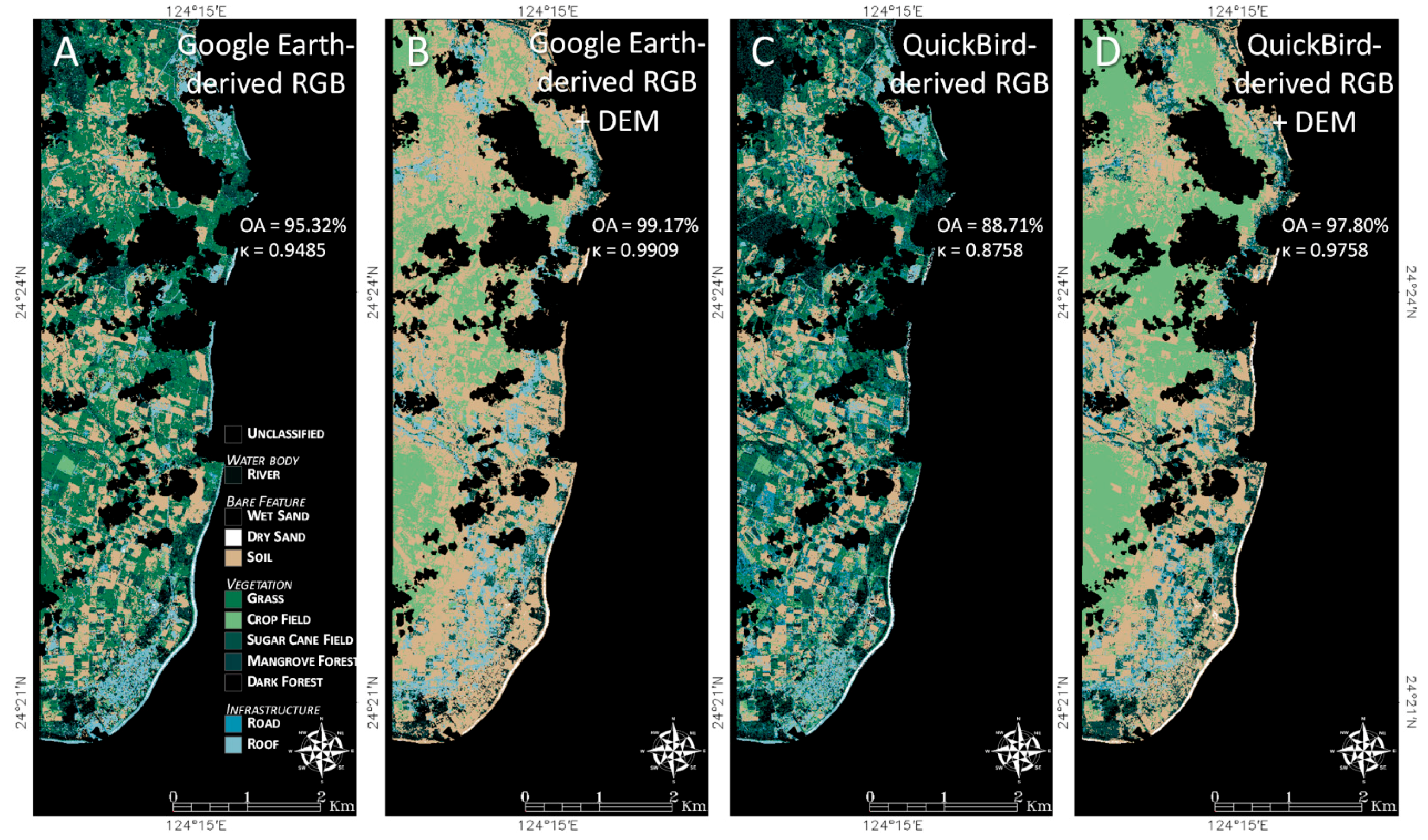
| Google Earth | QuickBird | |||||||
|---|---|---|---|---|---|---|---|---|
| RGB | RGB + DEM | RGB | RGB + DEM | |||||
| PA | UA | PA | UA | PA | UA | PA | UA | |
| River | 87.88 | 93.55 | 96.97 | 96.97 | 93.94 | 86.11 | 93.94 | 100 |
| Wet sand | 100 | 100 | 100 | 100 | 96.97 | 100 | 100 | 100 |
| Dry sand | 93.94 | 100 | 100 | 100 | 100 | 100 | 100 | 100 |
| Soil | 100 | 100 | 100 | 100 | 93.94 | 96.88 | 96.97 | 94.12 |
| Grass | 100 | 97.06 | 100 | 100 | 90.91 | 90.91 | 100 | 100 |
| Crop field | 100 | 100 | 100 | 100 | 100 | 94.29 | 93.94 | 100 |
| Sugar cane field | 96.97 | 100 | 100 | 100 | 100 | 94.29 | 100 | 100 |
| Mangrove forest | 96.97 | 88.89 | 96.97 | 96.97 | 48.48 | 64 | 100 | 94.29 |
| Dark forest | 96.97 | 91.43 | 100 | 100 | 78.79 | 76.47 | 100 | 100 |
| Road | 90.91 | 85.71 | 100 | 97.06 | 90.91 | 76.92 | 96.97 | 94.12 |
| Roof | 84.85 | 93.33 | 96.97 | 100 | 81.82 | 93.1 | 93.94 | 93.94 |
4. Discussion
4.1. Coastal Shallow Water Depth
4.2. Seamless Seabed and Land Cover Mapping
4.3. Limitations
5. Conclusions
Acknowledgments
Author Contributions
Conflicts of Interest
References
- Costanza, R.; d’Arge, R.; de Groot, R.; Farber, S.; Grasso, M.; Hannon, B.; Limburg, K.; Naeem, S.; O’Neill, R.V.; Paruelo, J.; et al. The value of the world’s ecosystem services and natural capital. Ecol. Econ. 1998, 25, 3–15. [Google Scholar] [CrossRef]
- Sukhdev, P. The Economics of Ecosystems and Biodiversity; European Communities: Wesseling, Germany, 2008. [Google Scholar]
- The Other 70% UNEP Marine and Coastal Strategy; UN-Gigiri: Nairobi, Kenya, 2011.
- Martínez, M.L.; Intralawan, A.; Vázquez, G.; Pérez-Maqueo, O.; Sutton, P.; Landgrave, R. The coasts of our world: Ecological, economic and social importance. Ecol. Econ. 2007, 63, 254–272. [Google Scholar] [CrossRef]
- Intergovernmental Panel on Climate Change (IPCC). Climate Change 2013—The Physical Science Basis: Working Group I Contribution to the Fifth Assessment Report of the Intergovernmental Panel on Climate Change; Stocker, T.F., Qin, D., Plattner, G.K., Tignor, M., Allen, S.K., Boschung, J., Nauels, A., Xia, Y., Bex, V., Midgely, P.M., Eds.; Cambridge University Press: Cambridge, UK, 2013. [Google Scholar]
- Adger, W.N.; Hughes, T.P.; Folke, C.; Carpenter, S.R.; Rockström, J. Social-ecological resilience to coastal disasters. Science 2005, 309, 1036–1039. [Google Scholar] [CrossRef] [PubMed]
- Cumming, G.S. Spatial resilience: Integrating landscape ecology, resilience, and sustainability. Landsc. Ecol. 2011, 26, 899–909. [Google Scholar] [CrossRef]
- Green, E.P.; Mumby, P.J.; Edwards, A.J.; Clark, C.D. Remote Sensing Handbook for Tropical Coastal Management; Edwards, A. J., Ed.; UNESCO Publishing: Paris, France, 2005. [Google Scholar]
- Landsat GeoCover ETM+ 2000 Edition Mosaics; USGS: Sioux Falls, SD, USA, 2004.
- GLSDEM, 90 m Scene GLSDEM_p123r024_utmz13; Global Land Cover Facility, University of Maryland: College Park, MD, USA, 2008.
- Liu, H.; Jezek, K.C. A complete high-resolution coastline of Antarctica extracted from orthorectified Radarsat SAR imagery. Photogramm. Eng. Remote Sens. 2004, 70, 605–616. [Google Scholar] [CrossRef]
- McClain, C.R.; Feldman, G.C.; Hooker, S.B. An overview of the SeaWiFS project and strategies for producing a climate research quality global ocean bio-optical time series. Deep Sea Res. II 2004, 51, 5–42. [Google Scholar] [CrossRef]
- MacMillan, D.; Bock, Y.; Fang, P.; Beckely, B.; Ma, C. Monitoring the TOPEX and Jason-1 microwave radiometers with GPS and VLBI wet zenith path delays. Mar. Geod. 2004, 27, 703–716. [Google Scholar] [CrossRef]
- Collin, A.; Archambault, P.; Planes, S. Bridging ridge-to-reef patches: Seamless classification of the coast using very high resolution satellite. Remote Sens. 2013, 5, 3583–3610. [Google Scholar] [CrossRef]
- Wang, L.; Sousa, W.P.; Gong, P.; Biging, G.S. Comparison of IKONOS and QuickBird images for mapping mangrove species on the Caribbean coast of Panama. Remote Sens. Environ. 2004, 91, 432–440. [Google Scholar] [CrossRef]
- Ghioca-Robrecht, D.M.; Johnston, C.A.; Tulbure, M.G. Assessing the use of multiseason Quickbird imagery for mapping invasive species in a Lake Erie coastal marsh. Wetlands 2008, 28, 1028–1039. [Google Scholar] [CrossRef]
- Dribault, Y.; Chokmani, K.; Bernier, M. Monitoring seasonal hydrological dynamics of minerotrophic peatlands using multi-date GeoEye-1 very high resolution imagery and object-based classification. Remote Sens. 2012, 4, 1887–1912. [Google Scholar] [CrossRef]
- Giri, C.; Ochieng, E.; Tieszen, L.L.; Zhu, Z.; Singh, A.; Loveland, T.; Masek, J.; Duke, N. Status and distribution of mangrove forests of the world using earth observation satellite data. Glob. Ecol. Biogeogr. 2011, 20, 154–159. [Google Scholar] [CrossRef]
- Gong, P.; Niu, Z.; Cheng, X.; Zhao, K.; Zhou, D.; Guo, J.; Liang, L.; Wang, X.; Li, D.; Huang, H.; et al. China’s wetland change (1990–2000) determined by remote sensing. Sci. China Earth Sci. 2010, 53, 1036–1042. [Google Scholar] [CrossRef]
- Guo, J.; Liang, L.; Gong, P. Removing shadows from Google Earth images. Int. J. Remote Sens. 2010, 31, 1379–1389. [Google Scholar] [CrossRef]
- Potere, D. Horizontal positional accuracy of Google Earth’s high-resolution imagery Archive. Sensors 2008, 8, 7973–7981. [Google Scholar] [CrossRef]
- Hu, Q.; Wu, W.; Xia, T.; Yu, Q.; Yang, P.; Li, Z.; Song, Q. Exploring the use of Google Earth imagery and object-based methods in land use/cover mapping. Remote Sens. 2013, 5, 6026–6042. [Google Scholar] [CrossRef]
- Mann, K.H.; Lazier, J.R.N. Dynamics of Marine Ecosystems: Biological-Physical Interactions in the Oceans, 2nd ed.; Blackwell Scientific Publications: Oxford, UK, 2006. [Google Scholar]
- Marine Biotic Survey (1989–1992) in the 4th National Survey on the Natural Environment: 1/10,000 Distribution Map of Coral Reefs; Environment Agency: Tokyo, Japan, 1996.
- Kayanne, H.; Harii, S.; Ide, Y.; Akimoto, F. Recovery of coral populations after the 1998 bleaching on Shiraho Reef, in the southern Ryukyus, NW Pacific. Mar. Ecol. Prog. Ser. 2002, 239, 93–103. [Google Scholar] [CrossRef]
- Lin, C.Y.; Wu, M.; Bloom, J.A.; Cox, I.J.; Miller, M.L.; Lui, Y.M. Rotation, scale, and translation resilient watermarking for images. IEEE Trans. Imag. Process. 2001, 10, 767–782. [Google Scholar] [CrossRef]
- Laben, C.A.; Brower, B.V. Process for Enhancing the Spatial Resolution of Multispectral Imagery Using Pan-Sharpening. U.S. Patent 6,011,875, 4 January 2000. [Google Scholar]
- Heyman, W.D.; Ecochard, J.L.B.; Biasi, F.B. Low-cost bathymetric mapping for tropical marine conservation—A focus on reef fish spawning aggregation sites. Mar. Geod. 2007, 30, 37–50. [Google Scholar] [CrossRef]
- Stumpf, R.P.; Holderied, K.; Sinclair, M. Determination of water depth with high-resolution satellite imagery over variable bottom types. Limnol. Oceanogr. 2003, 48, 547–556. [Google Scholar] [CrossRef]
- Collin, A.; Hench, J.L. Towards deeper measurements of tropical reefscape structure using the WorldView-2 spaceborne sensor. Remote Sens. 2012, 4, 1425–1447. [Google Scholar] [CrossRef]
- Congalton, R.G.; Green, K. Assessing the Accuracy of Remotely Sensed Data: Principles and Practices; Congalton, R., Green, K., Eds.; CRC Press: Boca Raton, FL, USA, 2008. [Google Scholar]
- Collin, A.; Planes, S. Enhancing coral health detection using spectral diversity indices from WorldView-2 imagery and machine learners. Remote Sens. 2012, 4, 3244–3264. [Google Scholar] [CrossRef]
- Smith, R.C.; Baker, K.S. Optical properties of the clearest natural waters (200–800 nm). Appl. Opt. 1981, 20, 177–184. [Google Scholar] [CrossRef] [PubMed]
- Hansen, M.C.; Potapov, P.V.; Moore, R.; Hancher, M.; Turubanova, S.A.; Tyukavina, A.; Thau, D.; Stehman, S.V.; Goetz, S.J.; Loveland, T.R.; et al. High-resolution global maps of 21st-century forest cover change. Science 2013, 342, 850–853. [Google Scholar] [CrossRef] [PubMed]
- Tachikawa, T.; Hato, M.; Kaku, M.; Iwasaki, A. Characteristics of ASTER GDEM Version 2. In Proceedings of the 2011 IEEE International Geoscience and Remote Sensing Symposium (IGARSS), Vancouver, BC, Canada, 24–29 July 2011.
© 2014 by the authors; licensee MDPI, Basel, Switzerland. This article is an open access article distributed under the terms and conditions of the Creative Commons Attribution license (http://creativecommons.org/licenses/by/4.0/).
Share and Cite
Collin, A.; Nadaoka, K.; Nakamura, T. Mapping VHR Water Depth, Seabed and Land Cover Using Google Earth Data. ISPRS Int. J. Geo-Inf. 2014, 3, 1157-1179. https://doi.org/10.3390/ijgi3041157
Collin A, Nadaoka K, Nakamura T. Mapping VHR Water Depth, Seabed and Land Cover Using Google Earth Data. ISPRS International Journal of Geo-Information. 2014; 3(4):1157-1179. https://doi.org/10.3390/ijgi3041157
Chicago/Turabian StyleCollin, Antoine, Kazuo Nadaoka, and Takashi Nakamura. 2014. "Mapping VHR Water Depth, Seabed and Land Cover Using Google Earth Data" ISPRS International Journal of Geo-Information 3, no. 4: 1157-1179. https://doi.org/10.3390/ijgi3041157
APA StyleCollin, A., Nadaoka, K., & Nakamura, T. (2014). Mapping VHR Water Depth, Seabed and Land Cover Using Google Earth Data. ISPRS International Journal of Geo-Information, 3(4), 1157-1179. https://doi.org/10.3390/ijgi3041157


