Article

Measuring Completeness of Building Footprints in OpenStreetMap over Space and Time

1
Leibniz Institute of Ecological Urban and Regional Development Germany, Weberplatz 1, Dresden 01217, Germany
2
Institute for Cartography, Dresden University of Technology, Helmholtzstr. 10, Dresden 01069, Germany
*
Author to whom correspondence should be addressed.
ISPRS Int. J. Geo-Inf. 2013, 2(4), 1066-1091; https://doi.org/10.3390/ijgi2041066
Submission received: 30 September 2013 / Revised: 29 October 2013 / Accepted: 30 October 2013 / Published: 11 November 2013

Abstract

:
Due to financial or administrative constraints, access to official spatial base data is currently limited to a small subset of all potential users in the field of spatial planning and research. This increases the usefulness of Volunteered Geographic Information (VGI), in particular OpenStreetMap (OSM), as supplementary datasets or, in some cases, alternative sources of primary data. In contrast to the OSM street network, which has already been thoroughly investigated and found to be practically complete in many areas, the degree of completeness of OSM data on buildings is still unclear. In this paper we describe methods to analyze building completeness and apply these to various test areas in Germany. Official data from national mapping and cadastral agencies is used as a basis for comparison. The results show that unit-based completeness measurements (e.g., total number or area of buildings) are highly sensitive to disparities in modeling between official data and VGI. Therefore, we recommend object-based methods to study the completeness of OSM building footprint data. An analysis from November 2011 in Germany indicated a completeness of 25% in the federal states of North Rhine-Westphalia and 15% in Saxony. Although further analyses from 2012 confirm that data completeness in Saxony has risen to 23%, the rate of new data input was slowing in the year 2012.

1. Introduction

1.1. Motivation

The launch of the OpenStreetMap (OSM) project in 2004 marked a new approach to the gathering and use of geodata. This project has been made possible by the increasing proliferation of GPS devices amongst private users and the availability of web-based mapping services offering high-resolution ortho-photographs. All data is provided under a free and open license—formerly Creative Commons Share Alike license (CC-BY-SA), today Open Database License (ODbL)—which, in general, makes this data easily accessible and usable. Organizations have to be aware of the legal aspects when mixing OSM data with commercial datasets. While work that is produced from OSM data, such as paper maps or mashups, can now expect to enjoy full copyright protection, geo databases that are derived from OSM need to be re-published under ODbL and, thus, any improvements made directly to the OSM dataset must be fed back into the project. Nevertheless, the increasing level of completeness and frequent updating of OSM data raises its potential value for diverse applications. One important attraction for many potential users is the financial savings which the OSM project offers. Thus, interest in OSM data is increasing not only in the private sector but also amongst Federal and regional agencies, the business sector as well as research institutes.
One potential field of application for OSM data is in spatial science. Against a backdrop of demographic change, climate protection and scarce resources, it is crucial to ensure the sustainable development of settlement structures. In order to realize the political goals of increased sustainability (e.g., minimizing land consumption, encouraging infill development, reducing CO2 emissions, and meeting targets for noise and air pollution), data is required that describes the built environment, especially the morphological structure of human settlements at a sufficiently high degree of resolution.
Alongside infrastructure, buildings constitute one of the most important physical elements of settlements, determining the morphological, functional, and socio-economic structure (type and form, land use, population patterns, energy needs, etc.). Currently there is a severe lack of relevant data describing the housing stock, such as its structure (e.g., function, age, size, form, physical arrangement, or material composition), parameters of use (e.g., number of households and resident population, energy consumption), and dynamics (e.g., demolition, new construction, conversion, renovation). The datasets produced by national mapping agencies often lack the level of detail required to answer all questions in spatial science. Factors that can hinder data gathering are meager financial resources, administrative constraints and, in some cases, strict laws on data privacy.
Automated approaches are being developed by spatial researchers to attempt to solve this problem by making use of geographic base data or remote sensing imagery to derive detailed information on settlement structure [1,2]. For example, the SEMENTA® (Settlement Analyzer) system developed at the Leibniz Institute of Ecological Urban and Regional Development can be used to analyze the morphology of building stock as well as to calculate various indicators describing the built environment such as building density, building coverage ratio, floor-area ratio, and housing or population density at urban block level, with resulting data visualized within a GIS [1]. It is intended to make the results freely available within the framework of a web-based information system for monitoring land use in Germany (www.ioer-monitor.de) [3]. The basic input data is in the form of building footprints taken from digital topographical data of cadastral land registers (in Germany: ALK, ALKIS®) or national topographic surveys (in Germany: ATKIS® Base DLM).
A wide variety of spatial data is available, but access to the data is limited due to high costs. Thus, detailed topographic spatial base data on buildings is currently only available to a limited group of all potential users in the field of spatial planning and research who may desire to use it. Therefore, one interesting question is to examine the extent to which OSM’s free, user-generated building data is suitable as input data for an automated analysis of settlement structure. The aim of this empirical study is to measure the completeness of OSM data on buildings by comparing it with official survey data for selected representative study areas. The focus of this study is the geometric completeness since it is suspected that the recording of semantic information of OSM buildings is even more incomplete than the geometry [4].

1.2. Related Work

Measuring the quality of spatial data is manifold. Data quality specification guidelines are subject of international standardization bodies such as ISO/TC 211. According to ISO 19157 (or 19113) data quality includes different elements (e.g., accuracy, resolution of data, integrity, logical consistency, or completeness). Completeness describes the presence or absence of features, their attributes and relationships [5]. To measure the completeness of Volunteered Geographic Information (VGI), usually the absence of features (also known as the omission error) is compared to a reference dataset. Here, different methods can be applied depending on the feature type (point, line, polygons). A very common way is to compute the total number (point features), total length (line features), or total area (polygon features) of all objects within a defined area and to compare it with a reference data set.
Previous studies on the quality of OSM data have largely focused on the completeness of the road network. Here, research on data completeness by Zielstra and Zipf [6], and Ludwig et al. [7] in Germany, by Haklay [8] in England, and by Zielstra and Hochmair [9] in the USA, have reached similar conclusions. Regardless of the choice of the reference dataset—TeleAtlas (today: TomTom) for Zielstra and Zipf, NAVTEQ for Ludwig et al. [7], Ordnance Survey for Haklay, TIGER and TeleAtlas for Zielstra and Hochmair—it could be shown that the road network in the investigated regions was represented to a high degree of completeness. Zielstra and Zipf, for example, report that already at the beginning of 2010 the total length of the road network as calculated from OSM data differed by only 7% from the figure given by the navigation data provider TeleAtlas. Furthermore, the total roadway length indicated by OSM data was increasing over time. A clear trend can be detected towards a high level of completeness in large cities in contrast to the patchy nature of datasets for small towns and rural communities. In some instances, OSM data for urban regions contains even more information than that of reference datasets. Corcoran et al. [10] identified that, in addition to demographic factors, this phenomenon may be explained by the nature of the growth of the OSM street network, which is governed by the spatial processes of an initial exploration and a subsequent densification of unmapped areas. Neis et al. confirm a high correlation between population density and data completeness [11]. Furthermore, by comparing datasets over a number of years (2007–2011), it becomes clear that the quantitative gaps between the various reference datasets and OSM data are becoming much less significant.
Some findings by Ludwig et al. [7], and Amelunxen [12], on the positional accuracy of OSM data should also be mentioned in this context. Ludwig et al. [7], have determined that 73% of all homologous street objects lie at a maximum distance of 5 m to the reference data (NAVTEQ), with a further 21% located within 10 m. Amelunxen confirms these results by reporting an average positional error of 11 m when OSM address data is compared to house coordinates of governmental land surveys. This last result may also be viewed as an estimation of the positional accuracy of OSM building data. In addition, Haklay et al. show that with time the average geometrical accuracy of OSM objects increases, if these are revised by several persons [13].
Feature types other than the road network have not been so well researched. An investigation of Points of Interest has been undertaken by Strunck [14]. Hauck [15] has studied the quality of postal code polygons generated by OSM, while Schoof [16] has compared the land cover polygons from OSM data with those of the digital landscape model ATKIS® Basis-DLM. To analyze the OSM data quality in France, Girres and Touya [17] compared the three OSM primitives (point, line, polygon) with a reference dataset. They considered the quality elements suggested by Kresse and Fadaie [5] to assess the OSM data quality and outlined a correlation of data completeness and the number of contributors in a specific area. Recently, Jackson et al. [18] were assessing completeness and positional accuracy of infrastructure-associated point data in OSM for a study area in Denver (CO, USA).
An initial indication of the level of completeness of OSM building data has been given by Höpfner [19] by investigating the OSM address dataset. It may be assumed that this dataset strongly correlates with the number of buildings. The relative proportion of addresses contained within the OSM dataset in comparison to the number of addresses stored by TeleAtlas (data from February 2011), is only 7.5%, according to Höpfner. Finally, some first concrete research results dealing with completeness of buildings in VGI have been given by Götz and Zipf [20], who estimate the relative proportion of building objects in Germany captured by OSM to be approx. 30% (data as of January 2012), a figure that is currently growing by approx. 1% per month. This estimate is based on data from official census data that, unfortunately, is not optimal for purposes of comparison as only main buildings are represented and not ancillary buildings. Thus, the completeness of the building dataset is estimated rather too optimistically. Confirmation of this is provided by a comparison of the current number of OSM building objects—approx. 6.5 million—with the approx. 50 million building polygons included in the official building polygons (Amtliche Hausumringe, HU), a nationwide authoritative geospatial data product, which includes all buildings of the German real estate cadaster. Here, the proportion of buildings captured by OSM is seen to be only 13% [4].
Apart from these initial attempts to estimate the completeness of building data by investigating the total number of objects, up to now there have been (in contrast to streets and addresses) no spatially differentiated studies on the completeness of the OSM building dataset. Therefore, it needs to be confirmed that building completeness patterns do not differ from other completeness investigations on other feature types. Furthermore, the strengths and weaknesses of different methods to measure completeness of building footprints have not been tested and discussed in detail. A study of the completeness of OSM buildings in Germany was carried out in 2012, which partly forms the basis for the current work at hand. Interested readers can find a comprehensive presentation of results in Kunze [21], and Kunze et al. [22].

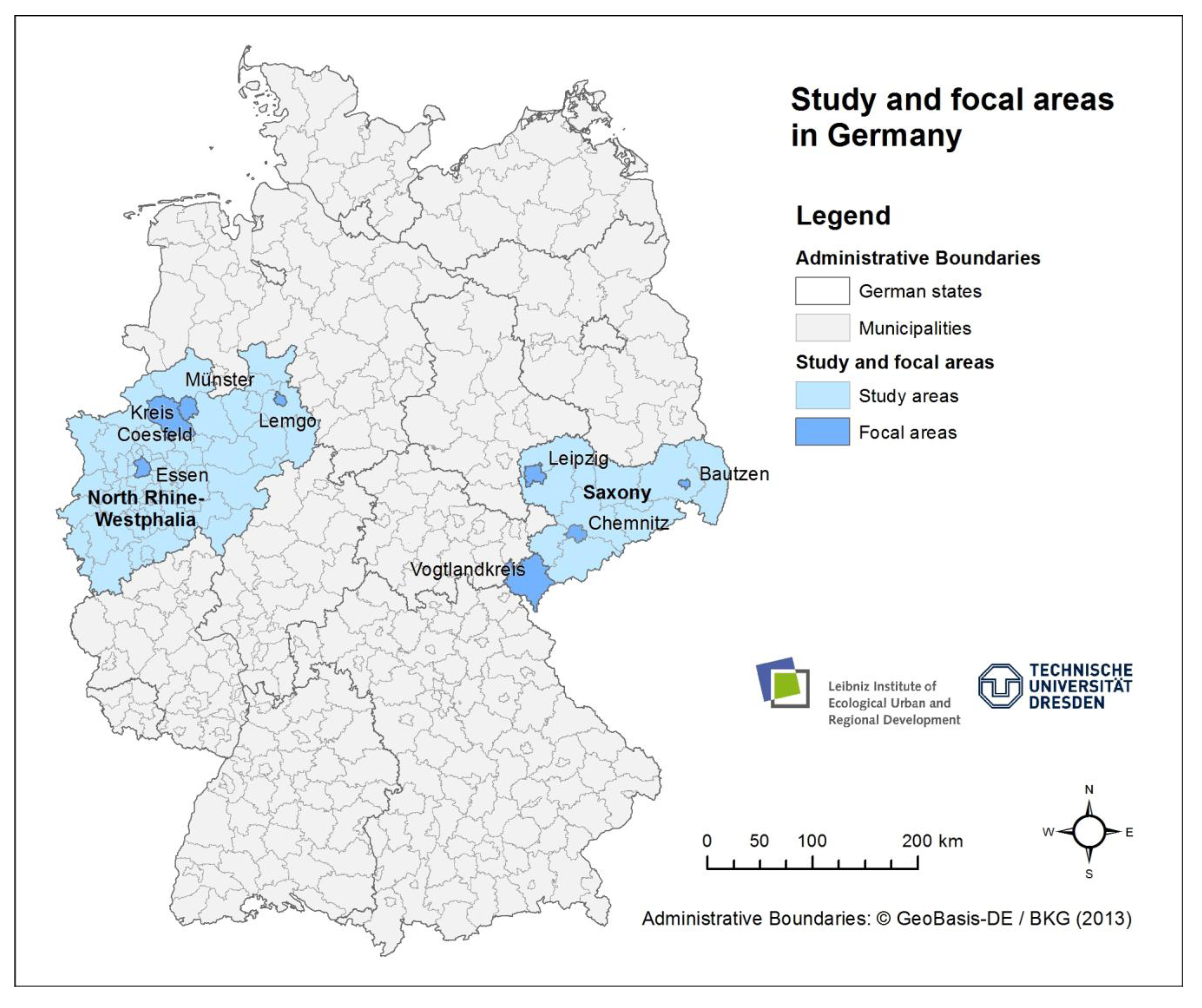
2. Study Areas, Datasets and Preprocessing

2.1. Study Areas

The areas selected for the study are the German states (Länder) of North Rhine-Westphalia (34,092 km2) and Saxony (18,419 km2). Combined, the two study areas cover 14.7% of Germany’s total area. For more detailed inspections, focal areas were chosen for both of these states based on the settlement structure types as defined by the Federal Institute for Research on Building, Urban Affairs and Spatial Development (BBSR) [23]. These are a representative city, a medium-sized town, a small town, and a rural region. For North Rhine-Westphalia these are Essen, Münster, Lemgo, and the rural district of Coesfeld (approx. 5.1% of the state’s total area), while in Saxony these are Leipzig, Chemnitz, and Bautzen, as well as the rural district of Vogtland (approx. 10.8% of the state’s total area) (Figure 1).
Figure 1. Study and focal areas in Germany.
Ijgi 02 01066 g001

2.2. Data Sets

In order to enable a comparative analysis, OSM data and an official reference dataset have been acquired for the study areas.
The OSM data as of 17 November 2011, 24 May 2012, and 5 November 2012, were supplied by the OSM service provider Geofabrik (www.geofabrik.de). Users can choose between different data formats: ESRI Shape-file, PBF, or OSM XML files, which differ in size and data complexity. It is possible to download whole countries or individual states as a data extract from the OSM database. Here, we made use of the Geofabrik download service in OSM XML format. In OSM, building data lacks standardization. Thus, objects and modeling rules are not defined. Buildings are usually represented with an outline (polygon), captured by different users through different data acquisition techniques and sources. For example, building data can be captured with the aid of handheld GPS-devices, through digitizing from aerial imagery (e.g., Bing, Mapquest), via measurements of sketch drawings from street level, or imported from government agencies databases (e.g., data import in France). Readers are advised to turn to Ramm et al. [24] for a comprehensive discussion of data capture within the OSM project. For these reasons, positional accuracy strongly depends on the acquisition technique. In particular, it depends on the geometric accuracy of the underlying primary source (resolution, distortion), the device used (low GPS accuracy) or the skills and experience of the user in sketching. Currently (August 2013), there are over 1.3 million registered members in the OSM project, but less than 2% (approx. 20,000) of these members continuously contribute to the project [25].
The official building polygon dataset (Amtliche Hausumringe) was used as a reference dataset. This German-wide dataset contains all building footprints from the cadastral agencies produced by the federal surveying and mapping authorities of the German States. The product is distributed nationwide by the Zentrale Stelle für Hauskoordinaten, Hausumringe (ZSHH) [26]. For the study area of North Rhine-Westphalia official building polygons as of 24 June 2011 (date of conflation) were adopted as reference data. The ALK (Automatisierte Liegenschaftskarte), which serves as the proof of all parcels of land and buildings in Germany, is the cadastral database for the derivation of the official building polygon dataset. Due to current building completeness issues within the ALK of the federal state of Saxony [27] building footprints from ATKIS® Base DLM, as of July 2011, were used as reference data. This is the nationwide Digital Landscape Model of the Authoritative Topographic Cartographic Information System (ATKIS) with a scale of 1:10,000–1:25,000 and contains all buildings in the same manner as in the official building polygon dataset (see definitions and mapping rules in Table 1).
Unlike OSM, modeling rules for buildings and their properties are clearly defined for datasets produced by national mapping and cadastral agencies. According to the Federal Statistical Office Germany (Destatis) and the Statistical Office of the European Commission (Eurostat) a building is defined as a “roofed construction which: can be used separately; has been built for permanent purposes; can be entered by persons; is suitable or intended for protecting persons, animals or objects” [28]. Furthermore, every building has a roof, but does not necessarily need walls (e.g., carports, shelters). A separate building is any free-standing building and in the case of interconnected structures (e.g., semi-detached or terraced houses), any unit separated from other units by a fire wall. The definition of a building in the official building polygon dataset and the databases of the federal surveying and mapping authorities of the German States (ATKIS® Base DLM) coincides with the definition from Eurostat; with the exception that underground constructions are excluded. Table 1 summarizes selected aspects of the used datasets.
Table 1. Overview of the datasets used.
OpenStreetMapReference Data
Official Building Polygons (North Rhine Westphalia)Buildings from ATKIS® Base-DLM (Saxony)
Building definitionNo definitionState specific building definition (e.g., § 2 of the State Building Code North-Rhine Westphalia [29]) corresponds to the definition from Eurostat, with the exception that only aboveground buildings are considered [26]Corresponds to the definition from Eurostat, with the exception that only aboveground buildings are considered, see definition in ATKIS [30]
Mapping ruleNo strict mapping rules, only recommendations, according to OSMWiki, that buildings can be mapped as individual buildings, the outline of building blocks or other complex arrangement of properties. If possible the outline should represent the outer edge of the wall [31] The characteristic outer edge of the wall of the building and/or the sharing firewall between interconnected buildings, see object type catalogue OBAK-LiegKat NRW [32]Complete recording of all buildings with addresses and all other buildings except very small buildings (e.g., shelters, garden sheds), see ATKIS [30]
Feature TypePolygonPolygonPolygon
Data capture processDifferent data acquisition techniques and sources: e.g., data from handheld GPS-device, digitizing from aerial imagery (e.g., Bing, Mapquest), data extractions and import by government agencies, observation from street level (e.g., sketch drawing, taking measurements)Derived database contains a copy of data from cadastral databases (e.g., ALK or ALKIS®) were buildings are captured through official surveying (Folie 11 in ALK) or mapping through large-scale maps or aerial imagery interpretation (Folie 84 in ALK)Digitized from digital orthophotos, terrestrial surveys or import from other authoritative data sources (e.g., surveying agencies of cities), see surveying office Saxony GeoSN [33]
Positional accuraciesDepending on acquisition technique (e.g., resolution of aerial imagery, distortion, GPS accuracy)planimetric accuracy of ±0.5 m, see [26]planimetric accuracy of ±3 m [30]
UpdatingContinuous updating Continuous updating of primary data bases (ALK), yearly updating of the derived official building polygon dataset Periodical updating, within maximally 3 years

2.3. Preprocessing

As mentioned above, there are different data formats available to obtain OpenStreetMap information and also several service providers which supply data extracts from countries or states. Besides the preprocessed “building” Shape-File from the Geofabrik download-service, it is possible to import the raw XML-File (.osm) and load it into the ESRI’s ArcGIS GIS environment. Therefore, we have chosen the freely available ArcGIS Editor for OpenStreetMap (esriosmeditor.codeplex.com). The advantage of this procedure is that the user has more control of additional semantic information (OSM-tags). Building polygons can be extracted by running a keyword search using the key “building”. All polygon-objects that are attributed with a value not NULL are considered as buildings. To ensure comparability we omit very small objects with an area smaller than 20 m2 in all datasets. These objects are mainly garages, sheds, or shelters, which are not represented in the official dataset ATKIS® Base-DLM.
In order to make a spatial comparison of the OSM building polygons with the reference buildings, it is necessary to harmonize the spatial reference by using a common coordinate system. We have chosen the projected Cartesian coordinate system DHDN/3-degree Gauss-Kruger zone 3 (EPSG Code 31467), which also serves as spatial reference for topographic mapping in Germany. As OSM data is based on the geographic coordinate system WGS84 (World Geodetic System 1984, EPSG Code 4326) a coordinate transformation has been applied.
Apart from the above mentioned preprocessing, no other filters have been applied to improve OSM data quality. In contrast to the work of Brando [34], no conspicuous wrong tagged polygons could be identified in the OSM datasets from Germany.

3. Methods to Analyze the Level of Completeness

In this section we present different methods that can be applied for a detailed investigation of the completeness of building footprints contained within OSM. All methods have one thing in common: they make use of a reference dataset regarded as complete.

3.1. Comparison of Quantities Based on Reference Areas (Unit-Based Method)

A simple method to analyze the completeness of OSM building footprints is to compute the total number of buildings and the total building area within a defined spatial unit (e.g., a meaningful geographical, administrative, or geometrical unit) and to compare it with the results gained from a reference dataset. The measurement to describe data completeness can be expressed as a ratio of the total figures or a relative proportion (percentage). Such unit-based measurements have been already applied to study completeness of other polygon feature types such “lakes” [17] or land use objects [16].
Visualizing the ratio in choropleth maps makes it possible to identify regions with a good or poor level of data completeness. Administrative divisions are commonly used in thematic mapping. These areas are hierarchical in nature, featuring categories such as municipality, county (administrative district) or state. The use of administrative units enables easy comparison with official statistical data, an approach particularly suited to large-scale analysis. However, there are some drawbacks in choosing such units for evaluating data completeness due to the Modifiable Areal Unit Problem (MAUP) [35], and the restricted comparability over time as unit boundaries shift. An evaluation of data completeness based on administrative units may also lack sufficient detail for a small-scale survey, for which smaller units are better suited.
In a geometrical approach the area can be divided into a regular raster of squares, triangles or hexagons. Hexagonal raster, such as employed in the recent work of Roick et al., offer the advantage (against squares and triangles) of more closely approximating the circle while providing the same complete coverage of the study area [36].
For local investigations, it is possible to use the methods of concentric circles around the center of cities or municipalities, or the buffering of municipality borders towards the center. This allows trends to be analyzed from the center to the periphery. Figure 2 gives an overview of the various spatial units.
Figure 2. Spatial units for analyzing completeness (modified after Kunze et al. [22]).(a) Geometrical raster (square, hexagonal); (b) Administrative units (municipalities); (c) Concentric circles; (d) Buffering of municipal borders.
Ijgi 02 01066 g002
It is necessary to compute the total numbers of buildings and the total building footprint area for both OSM and reference datasets. To ensure the correct calculation of the number of buildings, each building is reduced to its geometrical center (centroid) in order to avoid double counting within different spatial units.

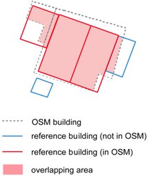
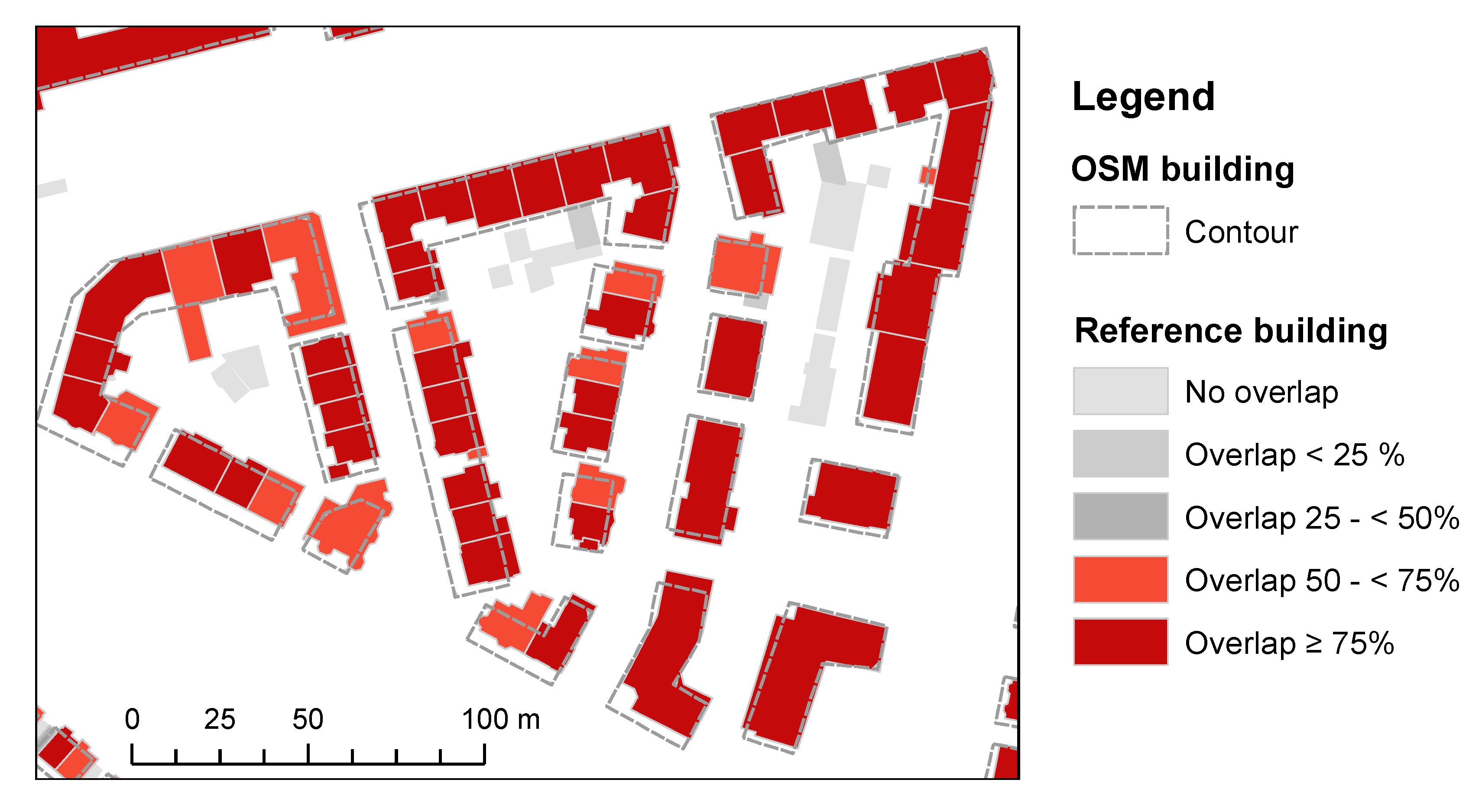
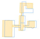
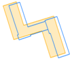
3.2. Comparison of Objects Based on the Centroid and Degree of Overlap (Object-Based Method)

In addition to a comparison of aggregate values, data completeness can also be analyzed by means of an object-based comparison. In this procedure homologous objects are investigated in both datasets. The specific question to be answered in the object-based method is: How many officially surveyed buildings are already represented in OSM? In order to determine this, it is necessary to test whether a building in the reference dataset is represented by an object in the OSM dataset. For this purpose, automated matching of homologous buildings must be carried out.
In the literature, many matching algorithms based on similarity measures have been proposed (e.g., [37]). Here, we propose two basic object-based methods, namely the centroid method and the overlap method (Table 2). The centroid method is based on a spatial query resulting in an answer as to whether the geometrical center of a reference polygon lies within an OSM polygon. If so, the criterion is successfully met. In this study, common “Feature to Point” function from ESRI ArcGIS 10.0 with the INSIDE option has been used. The overlap method, formerly used in building-based change detection [1], may be understood as a combination of a topological query and an overlap operator. The criterion for agreement is met when the common area of overlap between the two polygons is at least half as large as the total area of the reference polygon, corresponding to an overlap degree of 50%. Figure 3 presents a color-coded visualization of the degree of overlap of officially surveyed buildings, ranging from grey (no overlap) to dark red (high degree of overlap).
Figure 3. Color-coded illustration of degree of overlap between building footprints in official and OSM datasets.
Ijgi 02 01066 g003

3.3. Overview of the Tested Methods

Table 2 summarizes the methods introduced in the last two sections. The completeness in regard to reference areas (unit-based methods) is computed in terms of the number of buildings CNo and the building area CArea. These are very basic measurements, which probably tend to over- or underestimate the completeness due to aggregation at unit-level. Object-based approaches most likely provide more reliable measurements since they are not simply a comparison of statistical values. Their use avoids the potential drawbacks of the aggregation methods in which differences in modeling can distort results (Section 3.4). The level of data completeness in object-based approaches is determined as a proportion of the matched reference buildings to the total set of buildings. However, an object-based comparison also allows the completeness of areal coverage to be measured in relation to a specified reference area. In this case, differences in modeling may lead to artifacts in the measurements. Such an approach is, however, not applicable in many cases as the building footprint areas of OSM buildings do not necessarily correspond to those of the reference buildings.
Regarding the centroid method, artifacts in computing completeness may arise when buildings are grouped together rather closely and when building footprints differ in terms of degree of detailing, for example in the case of buildings with interior courtyards. The overlap method may avoid the mentioned drawback of the centroid method, as homologous buildings, which show a considerable locational shift between datasets and thus small area of overlap, will be ignored by this method.
In order to compare the strengths and weaknesses of these different measures of completeness, they were applied to real datasets. In the following it will be investigated whether a theoretical advantage of the overlap approach in comparison to the centroid approach can be confirmed.
Table 2. Methods to analyze data completeness.
Unit-Based ComparisonObject-Based Comparison
Centroid MethodOverlap Method
Ijgi 02 01066 i001 Ijgi 02 01066 i002 Ijgi 02 01066 i003
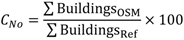
The proportion of the total number of OSM buildings and the reference buildings per unit in %.The proportion of the total number of reference buildings that are represented in OSM in %. The centroid of a reference building should intersect an OSM building.The proportion of the total number of reference buildings that are represented in OSM in %. At least 50% of the reference building footprint area should overlap an OSM building.
Ijgi 02 01066 i004 Ijgi 02 01066 i005 Ijgi 02 01066 i006
Proportion of the total area of all OSM buildings and the reference buildings per unit in %.

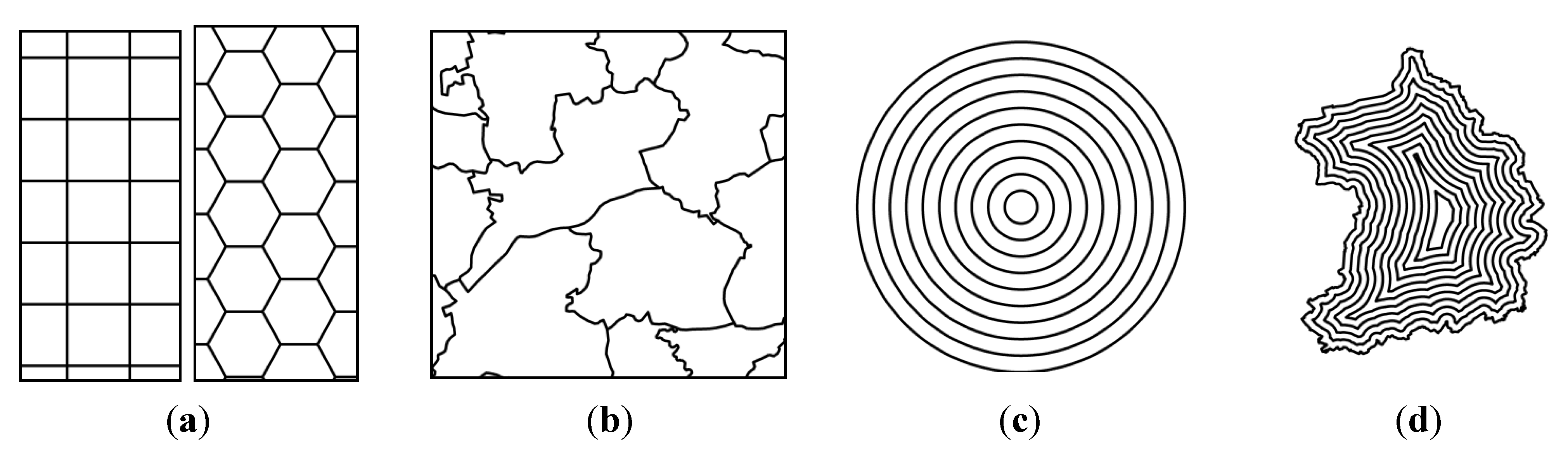
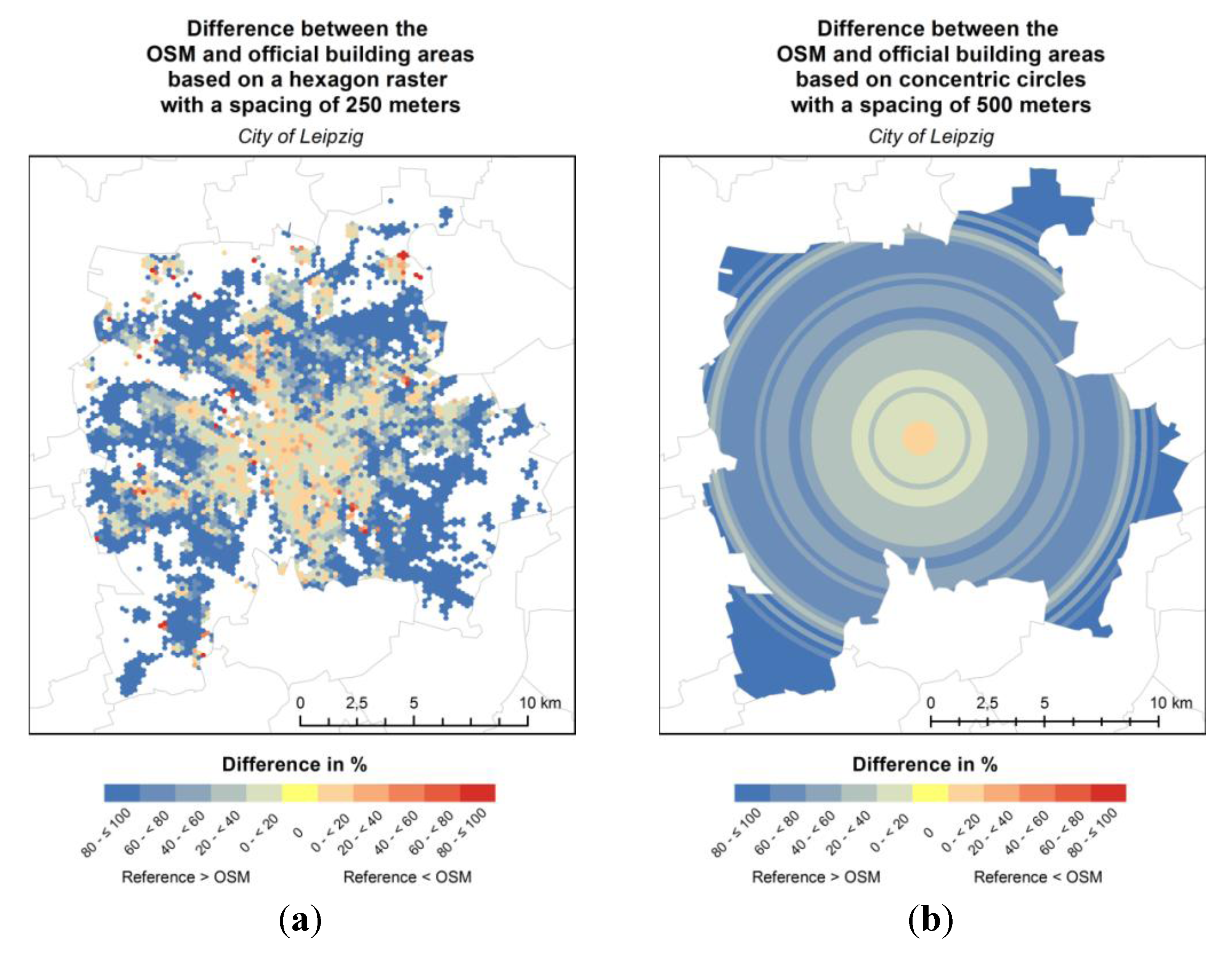
3.4. Cartographic Visualization of Data Completeness Patterns

The methods of administrative and geometrical units discussed in Section 3.1 not only aid the analysis of data completeness but also the visualization of results. One way of illustrating the degree of completeness is to visualize the disparity between building numbers or areas using a regular raster and a color-coded scale.
Figure 4 gives an example of such visualization for the City of Leipzig in Saxony, Germany. A high degree of detail is offered by the hexagonal raster with a spacing of 250 m (Figure 4a). The blue areas, primarily in rural districts, indicate cells where the total area of officially surveyed buildings is larger than the total area of OSM building objects (comparison on raster unit). In agglomerations the result is in some cases the opposite. The causes of this effect are explained more precisely below.
Zielstra and Zipf have already confirmed the link between the level of completeness of OSM street data and the distance to the city center [6]. An analysis of the completeness of OSM buildings, analyzed by means of reference areas in the form of concentric circles also confirms this relationship, as shown in Figure 4b. In this example, rings of width 500 m are shown. Only in Leipzig’s city center do we find the total area of OSM buildings exceeding that of official surveyed data. Moving further away from the city center the discrepancy between the two datasets becomes ever greater, with building area calculated from the official dataset increasing over OSM data. These examples show how cartographic visualization techniques can help to identify different patterns of data completeness.
Figure 4. Cartographic visualization using (a) a hexagonal raster with a spacing of 250 m or (b) concentric circles with a spacing of 500 m (Figure 4b reproduced with permission from Kunze et al. [22]).
Ijgi 02 01066 g004

4. Results of the Completeness Analysis

In this section selected results of the completeness analysis are presented for various regions in Germany. These include the results of a comparison of the different methods as well as a multi-temporal analysis of the tested regions. The results were partly abstracted from [22] and compared to current OSM data in a multi-temporal analysis.
The four methods already discussed to examine completeness were employed to evaluate OSM building data. The authoritative data described in Section 2.2 as of 2011 was available as a reference dataset in all cases.

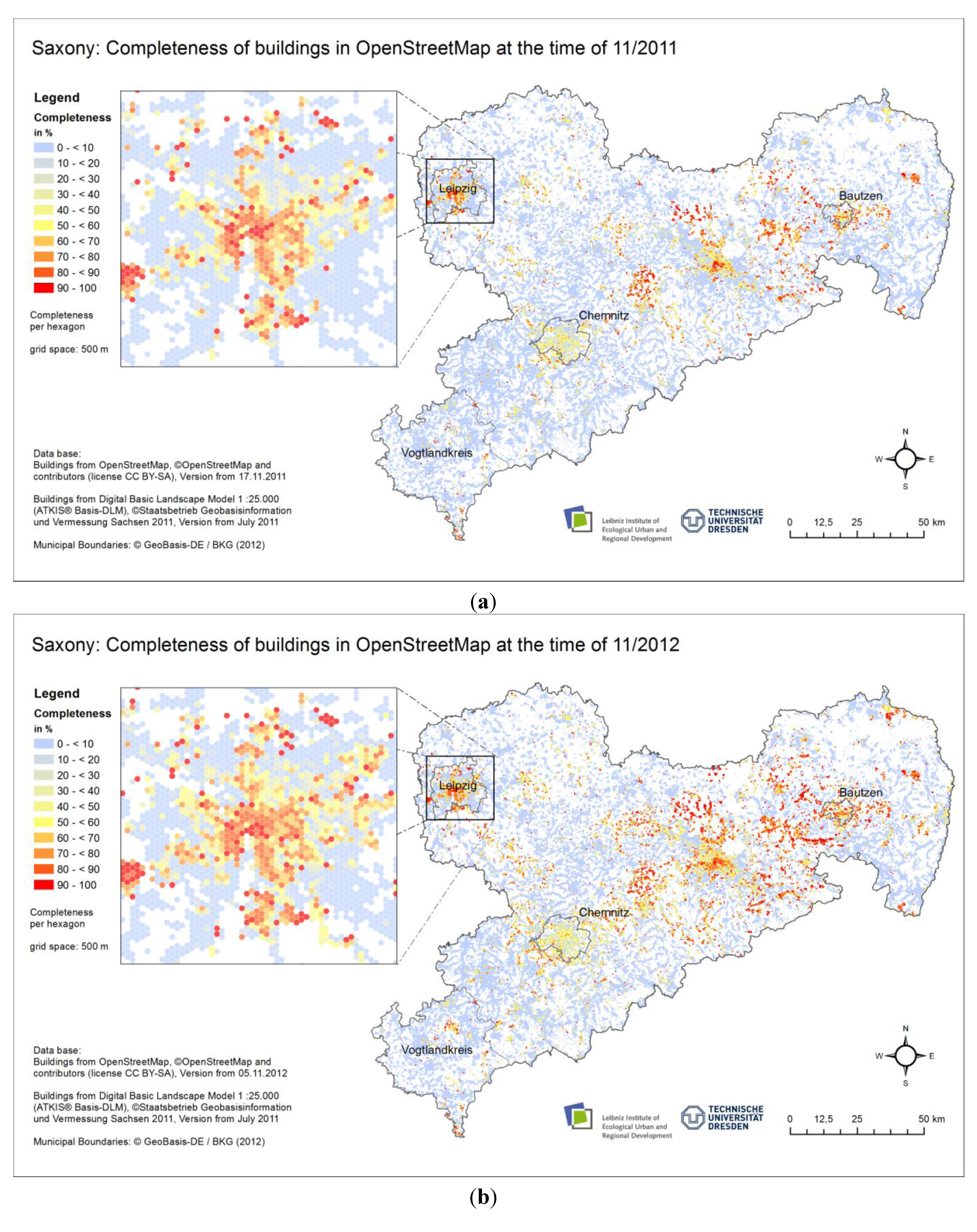
4.1. Completeness of OSM Buildings at Present

An overview of the results of the investigations into data completeness, broken down according to method used, is given in Table 3. The total number of reference buildings was 1,891,544 in Saxony and 8,887,495 in North Rhine-Westphalia.
Examining the unit-based methods we find large disparities in OSM data completeness based on the number of buildings and the building area. The explanation for this is the previously discussed variations in the modeling of building polygons both in the OSM and the reference dataset. Regarding calculations for number (CNo), the degree of completeness is underestimated, as officially surveyed buildings are generally captured at a higher degree of resolution. In particular, detached buildings or building complexes with many parts are not captured in sufficient detail within OSM, leading to a much lower number of buildings detected per unit area. It can be assumed that any estimates of the completeness of building areas (CArea.) will tend to be too high. As OSM buildings are generally digitized from ortho-images, they frequently represent the roofing area rather than the floor plan, as in the reference footprint outlines. The higher degree of completeness indicated for building area is, however, generally due to the lower degree of resolution in the representation of complex structures, as can be seen in first figure in Section 5.1, where the interior courtyard is not modeled.
The result of data completeness using object-based approaches indicates the relative proportion of officially surveyed buildings represented by a corresponding building in the OSM dataset. The values for CCentr and COverlap differ only rarely by more than one percentage point, and generally fall between the two extreme values of the reference area methods. It is thus clear that modeling discrepancies only have a minor impact on object-based analysis. Using these methods, a degree of completeness of over 50% is achieved for the city of Essen, compared to less than 2% for the small town of Lemgo.
With reference to the object-based approaches, completeness is seen to be rather poor in rural areas, where less than one quarter of buildings is represented in OSM data (Table 3). One explanation for this is that the low population density in such areas results in a small number of active OSM mappers. This contrasts with the example of towns with only a small population, where few highly active mappers are found (e.g., Bautzen). A comparison between cities in Saxony and North Rhine-Westphalia also reveals some differences. For example, the object-based analysis of completeness for Essen indicates a share of buildings captured by OSM of over 50%, whereas in Leipzig the completeness is just under 30%.
Table 3. Results of investigations on completeness of OSM buildings as of 17 November 2011 using the four described methods (data previously published in Kunze et al. [22]).
Unit-Based MethodObject-Based Method
SaxonyNo. of Buildings in ReferenceCNo (%)CArea. (%)CCentr (%)COverlap (%)
Leipzig (large city)119,15825.258.828.928.4
Chemnitz (medium-sized town)104,98724.360.432.031.4
Bautzen (small town)15,22337.480.847.844.5
Vogtlandkreis (rural district)115,9306.515.64.94.5
Entire State1,891,54414.530.715.314.4
North Rhine-WestphaliaNo. of Buildings in ReferenceCNo (%)CArea. (%)CCentr (%)COverlap (%)
Essen (large city)163,42730.984.153.552.5
Münster (medium-sized town)117,3935.528.18.88.7
Lemgo (small town)25,0021.213.01.81.7
Kreis Coesfeld (rural district)150,9339.421.410.59.6
Entire State8,887,49515.645.925.024.3
The level of completeness indicated by the overlap method falls slightly below that determined by the centroid method. For North Rhine-Westphalia the difference is striking: 25.0% (CCentr) and 24.3% (COverlap). By examining diverse cases it becomes clear that both methods have certain advantages and disadvantages. The process of abstracting the reference building to a single point in the centroid method can lead to errors in building identification, and thus a slight over- or under-estimation of the level of completeness. On the other hand, differences in the representation of building size in combination with a locational shift can lead to identification errors in the overlap method. Thus, while the centroid in the reference building may correspond to that of the OSM building, it may be that the overlap between the corresponding polygons is less than 50%. In the case of North Rhine-Westphalia, this results in an underestimation of the level of OSM data completeness using the overlap method.

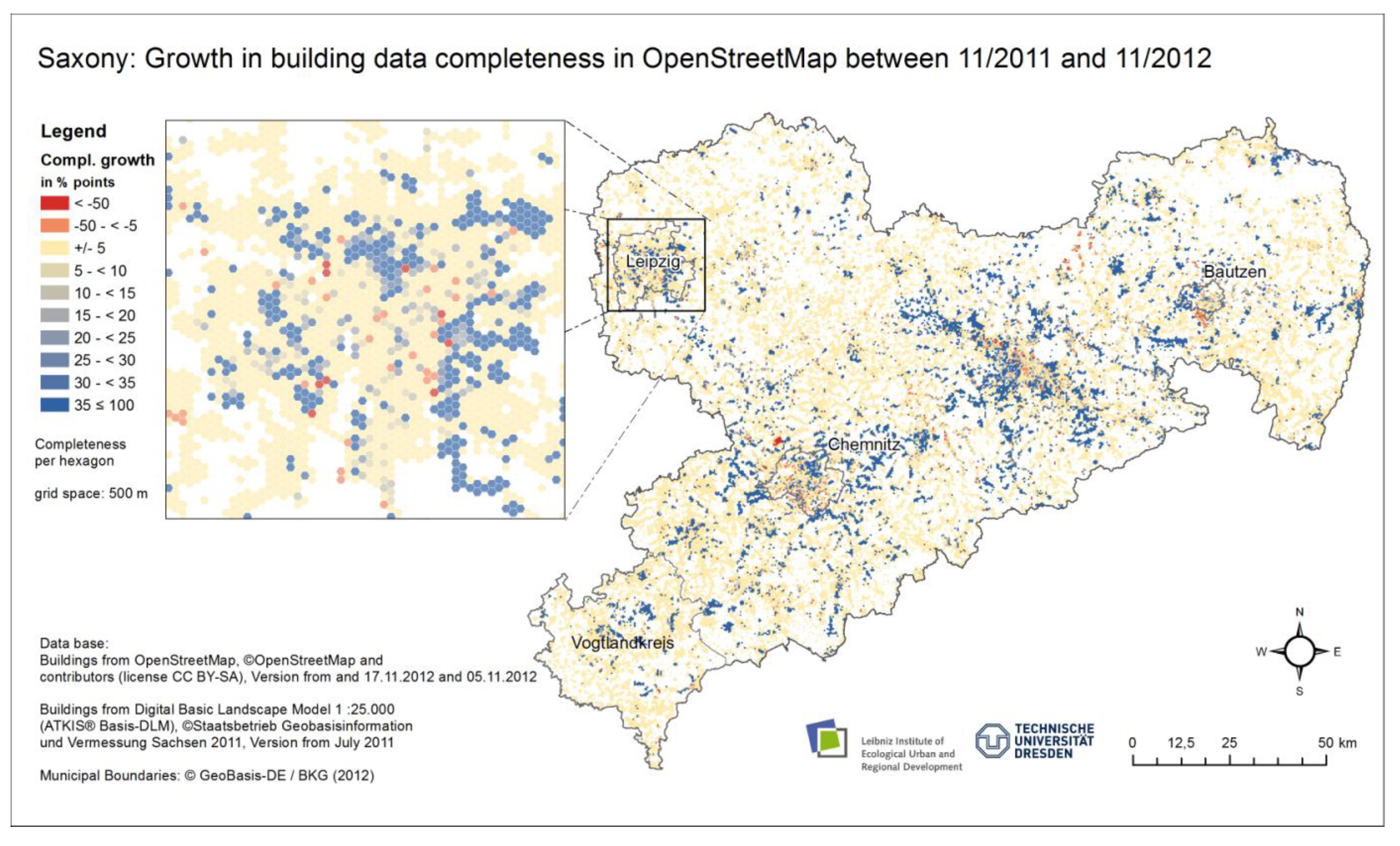
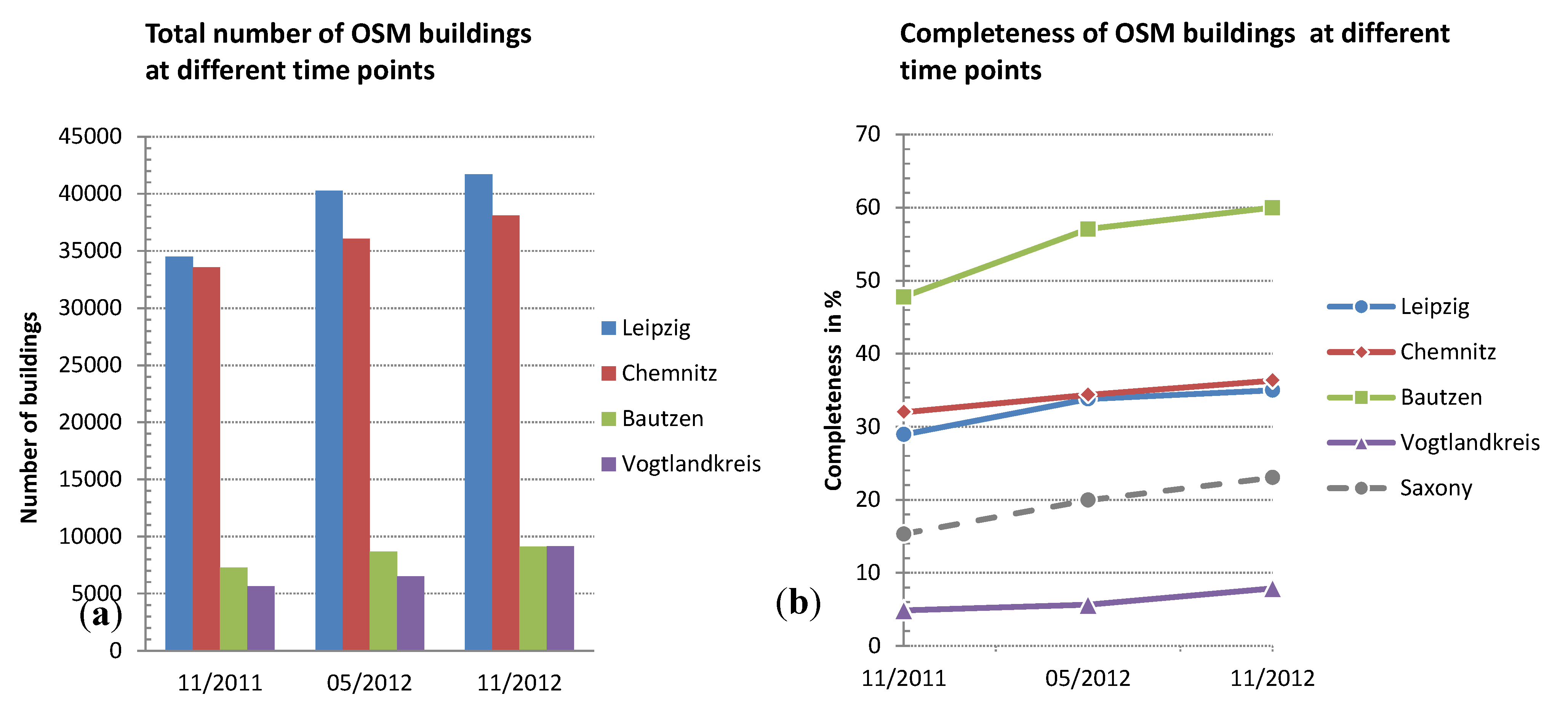
4.2. Growth in Completeness of OSM Buildings over Time

In order to study data completeness over time, three OSM datasets were considered at different time points (Section 2.2). The building footprints from the official German topographic database ATKIS® Base DLM, as of July 2011, serve as the reference for all comparisons (Table 4). Changes in the building stock have been neglected in this study due to the very short period under observation.
Table 4. Summary of the results of the multi-temporal analysis.
Completeness in % at Different Time PointsDifference in Percentage Points (p.p.)Completeness Growth Rate p.a. in %
Temporal Reference17 November 201124 May 20125 November 2012b/t 1st and 3rdb/t 1st and 3rd
Number of Buildings (Unit-Based Method)
Saxony14.519.722.88.356.8
Leipzig25.229.630.75.521.7
Chemnitz24.326.228.03.815.6
Bautzen37.447.448.110.728.6
Vogtlandkreis6.58.512.25.685.6
Sum of Building Area (Unit-Based Method)
Saxony30.737.641.711.035.9
Leipzig58.865.768.49.616.3
Chemnitz60.466.470.39.916.3
Bautzen80.891.592.711.914.7
Vogtlandkreis15.618.723.17.548.4
Number of Buildings (Centroid Method)
Saxony15.320.023.07.750.6
Leipzig28.933.835.06.120.9
Chemnitz32.034.436.34.313.5
Bautzen47.857.160.012.225.5
Vogtland4.95.67.93.061.8
Number of Buildings (Overlap Method)
Saxony14.418.822.27.753.8
Leipzig28.433.134.56.221.8
Chemnitz31.433.735.84.414.0
Bautzen44.553.157.813.330.4
Vogtland4.55.17.22.759.6
Figure 5 shows the rise in data completeness for Saxony over time in terms of the total number of buildings and the level of completeness expressed as a percentage. Here, the object-based centroid method was employed for the comparison.
Figure 5. Increase of completeness over time (centroid method) in Saxony: (a) total number of buildings and (b) level of completeness in percent.
Ijgi 02 01066 g005
Table 4 summarizes the results of applying all methods, showing data completeness at the different time points as total datasets as well as expressed as percentage points (p.p.) and the completeness growth rate. The latter indicator is defined as the proportionate growth in completeness per year (p.a.) in percent. It can be seen that the total number of captured buildings in the state of Saxony increased by approx. 57% in the period from November 2011 to November 2012. In the first half-year, more buildings were added to the database than in the second half year (approx. 100,000 and 60,000 respectively). In the second half year a decrease in the growth rate is detected in all test areas, with the exception of “Vogtlandkreis”, which shows a proportionate increase in completeness of 85%, compared to the previous year.
Although, in this case, the growth rate of completeness is higher for the rural district of Vogtlandkreis, nevertheless the level of data completeness in urban areas greatly exceeds that of rural areas. The motivation of mappers to capture buildings in so far “unmapped” areas seems to be greater than in already mapped areas. On the other hand it is harder to complete missing buildings in large areas which already have good coverage. These findings correspond to those of Corcoran et al. who found that the growth of data on the street network is governed by an initial exploration into unmapped areas followed by a subsequent densification [10].
Figure 6a,b show completeness maps of OSM buildings in the state of Saxony for November 2011 and November 2012, while the growth rate in completeness is shown in Figure 7.
Figure 6. Visualization of the completeness of OSM buildings in the Federal State of Saxony as of (a) November 2011 and (b) November 2012.
Ijgi 02 01066 g006
Figure 7. Visualization of the completeness growth rate of OSM buildings in the Federal State of Saxony between November 2011 and November 2012.
Ijgi 02 01066 g007

5. Sources of Error in Measuring Completeness

In this section, various factors are discussed which influence the determination of completeness. One challenge is the varying degree of abstraction within OSM. Such discrepancies can be uncovered by analyzing the object-to-object cardinalities. Another problem is the positional mismatch between buildings of different data sources.

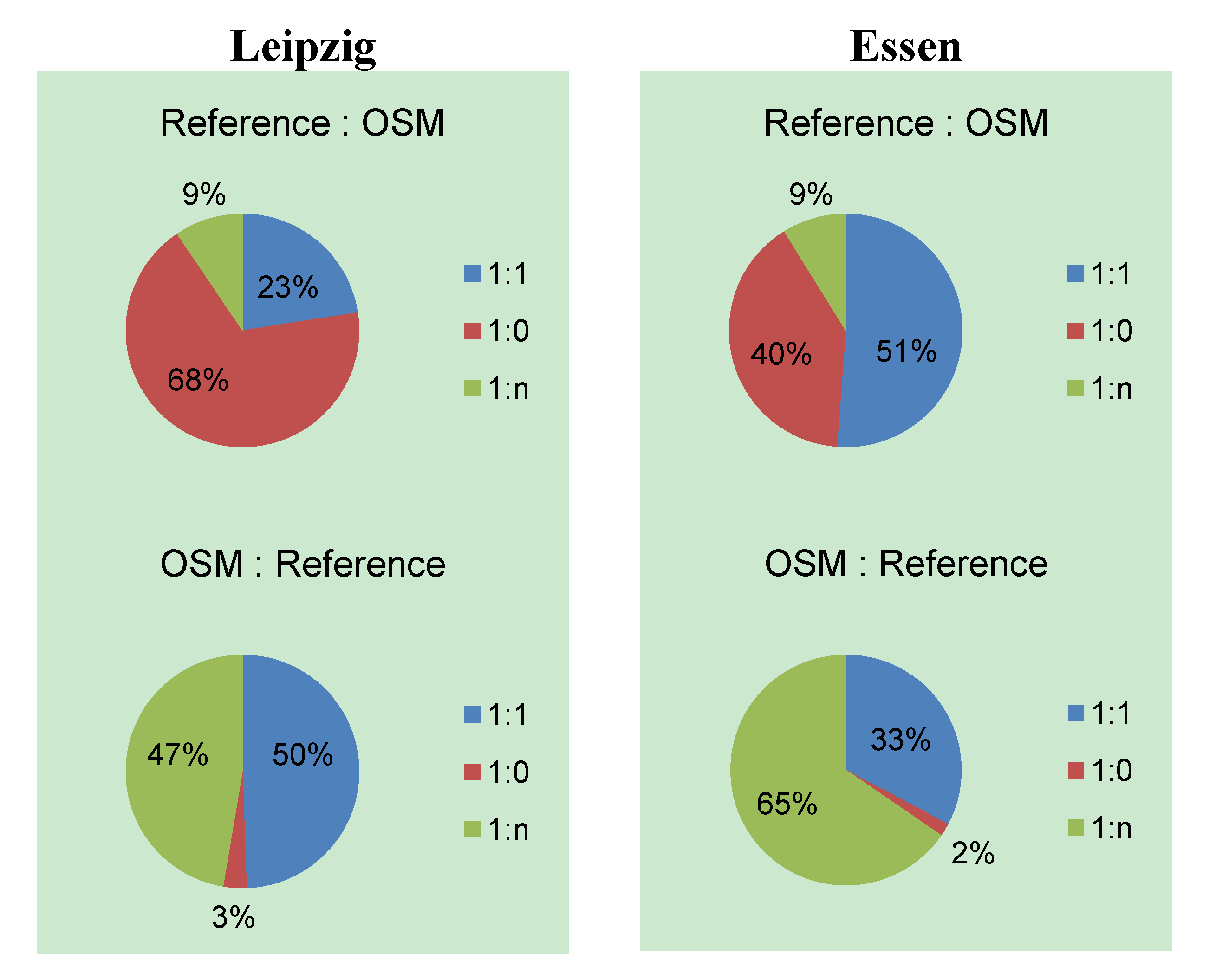
5.1. Discrepancies in Modeling

Completeness rates based on building numbers or areas (unit-based method) are greatly influenced by the quality of the building polygons. OSM buildings are in part heavily generalized during acquisition by OSM mappers. This can be due to a lack of conventions for the representation of buildings, perhaps poor input data for the digitization process, and also to some extent a lack of sufficient motivation amongst the OSM community to ensure a detailed representation of buildings. Often individual buildings are merged into one object. Clearly in the case of terraced housing any calculation of the total number of houses will greatly depend on whether such houses are modeled as individual buildings or as a single block. The calculation of building area can also vary greatly according to the degree of abstraction, for example in the case of buildings with an interior courtyard. This is made clear in Figure 8.
Figure 8. Different approaches to polygon modeling.
Ijgi 02 01066 g008
One way to investigate the impact of these modeling discrepancies is to analyze the cardinality of represented buildings between the two datasets in direct object-to-object comparison. Table 5 shows the various typical ratios which can be determined between the officially surveyed polygons and the OSM building polygons, as well as their interpretations.
Table 5. Object-to-object cardinalities and their interpretation.
1:11:01:n
Ijgi 02 01066 i007 Ijgi 02 01066 i008 Ijgi 02 01066 i009
The building in the reference dataset corresponds to one building in the target datasetThe building in the reference dataset does not correspond to any building in the target datasetThe building in the reference dataset corresponds to several (n) buildings in the target dataset
n:m0:1n:1
Ijgi 02 01066 i010 Ijgi 02 01066 i011 Ijgi 02 01066 i012
Several (n) buildings in one dataset correspond to several (m) buildings in the other datasetNo building in the reference dataset corresponds to a building in the target datasetSeveral (n) buildings in the reference dataset correspond to one building in the target dataset
The modeling differences revealed by the ratios 1:n, n:1, and n:m strengthen the argument for the use of the object-based centroid and overlap methods against the calculations by means of reference area. In the case of 1:n the additional problem arises that it is impossible to link dataset objects using the centroid method if no OSM polygon exists at the same position as the reference centroid, even if OSM building footprints are available for the rest of the reference building area. This case only arises if OSM data has a higher degree of resolution than the buildings of the reference dataset.
Figure 9 presents the results of the data analysis for two selected focal areas in the form of simple cardinalities. The incomplete nature of OSM building data is reflected here in the numerous 1:0 cardinalities between official datasets and OSM objects. Around 50% of the building objects in the test area of Essen show a 1:1 relationship, indicating a good representation of buildings within OSM. In Leipzig, however, only about one quarter of officially surveyed buildings can be matched to OSM buildings. These figures correspond with the results of the object-based comparative methods to determine data completeness.
Figure 9. Object relation between reference buildings and OSM buildings for the focal areas Leipzig and Essen.
Ijgi 02 01066 g009
The cardinalities considered in the opposite direction, by matching OSM buildings to officially surveyed objects, are also shown in Figure 9. Here differences can once again be discerned between Leipzig and Essen. The ratio 1:n occurs more frequently in Essen than in Leipzig, in contrast to the relationship 1:1, which occurs more often in Leipzig than in Essen. The explanation for this is that terraced housing is more common to Essen, which in the case of insufficiently detailed modeling in OSM favors the cardinality 1:n. Modeling errors in the reference dataset compound this problem. In Essen the building footprints derived from the ALK as reference dataset show a high degree of detail. Due to generalization many buildings represented in the ATKIS® Basic DLM of Leipzig are not modeled as individual buildings but rather as housing blocks. Thus the more prominent 1:1 ratio in the test area of Leipzig is not due to better modeling of OSM buildings, but rather a similar degree of abstraction in the reference dataset. Buildings represented in cadastral data are thus better suited for comparative investigations than building footprints from digital landscape models, primarily used for the production of topographic maps.

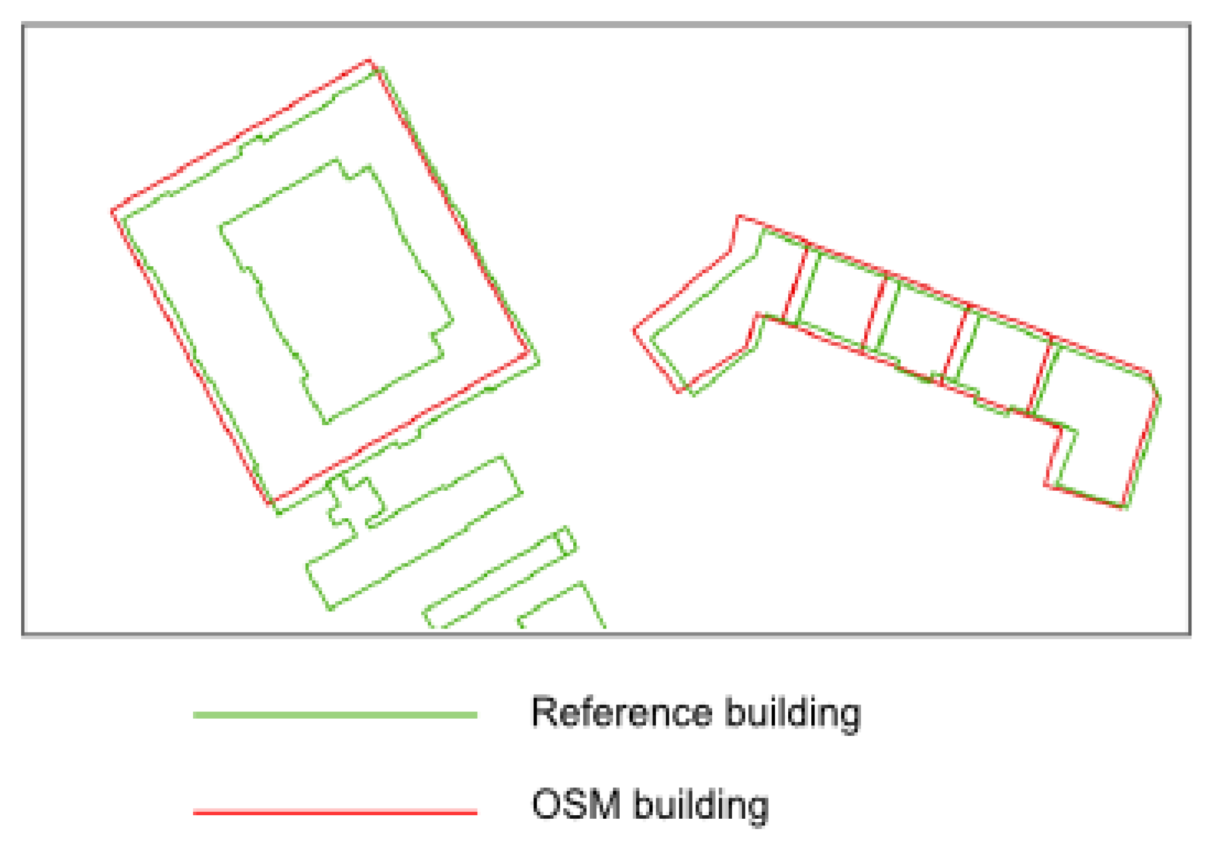
5.2. Positional Mismatches

Besides the lower degree of abstraction within OSM, the quality of the completeness measurements is also dependent on the positional accuracy. Using an object-based approach the detection of corresponding buildings forms the basis for the calculation of data completeness. Object-based methods are much less affected by differences in modeling. Yet, the centroid and overlap methods are more susceptible to errors caused by the spatial shifting of objects. Such shifts in OSM may be due to a number of factors, discussed, e.g., by Fairbairn and Al-Bakri [38]. As OSM buildings are usually digitized from satellite or aerial imagery, inaccuracies mostly occur because of insufficient resolution of imagery, radial displacements of roofing in ortho-images or erroneous rectification of ortho-images. An object-based matching procedure [39] that looks at building characteristics could serve to minimize these misallocations. A valid mutual linking of homologous buildings could form the basis for a transfer of attributes in both directions, and thus enhance official building data with semantic information taken from OSM buildings.

6. Conclusions and Outlook

6.1. Conclusions

VGI Data quality and data completeness of OSM data in particular have been widely studied within the geographic information science community in the last couple of years. Most of the previous studies focus on the completeness of the street network, whereas the completeness of buildings has not been studied in detail. First estimates on the completeness of buildings in OSM have been based on total statistics on a national level, which gives only a rough idea of completeness. Only by taking spatial differentiation into account are we able to confirm that completeness pattern of buildings are similar to those of other OSM feature types. To ensure data quality assessment of OSM data, the building completeness needs to be measured accurately by means of suitable reference building data, preferably building footprints taken from digital topographic databases.
We have introduced and discussed four different methods to determine the level of data completeness. Unit-based methods are based on the comparison of building numbers or building areas calculated for reference areas. Object-based methods, namely the centroid and overlap method, are based on the identification of corresponding buildings in both datasets.
From a methodological point of view, the following conclusions can be drawn. Unit-based methods of aggregating the numbers and areas of buildings per spatial unit require less computational efforts but show limitations in their level of detail. The results for this method indicate that a unit-based comparison of the total number or area of buildings is highly sensitive to disparities in modeling. Therefore, applying unit-based methods may result in huge over- or underestimation of completeness. The impact of modeling differences is lower for object-based methods, which are, on the other hand, more sensitive to positional mismatches of the OSM buildings. Therefore, we strongly recommend using object-based comparison. A conclusion as to which of the two object-based methods is best cannot be made on the basis of current data. This would require a detailed examination of the various types of errors that arise when matching buildings between two datasets. However, the difference between the centroid and overlap method is below one percentage point in all investigated areas. Since the centroid method is more efficient in computation, it is therefore the authors’ opinion that the centroid method is best suited.
The methods have been applied to various test areas in Germany. The following basic conclusions can be drawn from the analysis of building completeness. Building data from OSM, as of November 2012, is characterized by a low degree of completeness (clearly below 30%) and a strong heterogeneity in the geometrical modeling of buildings. Completeness is higher in urban than in rural areas and clearly decreases with increasing distance from urban centers. These completeness patterns are classic and similar to those of other feature types like the street network. However, for the first time, we could gain reliable information on the absolute completeness, which is far lower than expected and lower than for other feature types. The annual increase in completeness is relatively high but shows considerable spatial variation. For Germany as a whole, Götz [4] has forecasted that a similar level of completeness will be achieved for buildings as for street objects in around four to six years if the current speed of data capture is maintained. The results of our temporal analysis suggest a lower speed of data completion. Even if the detected deceleration in data integration is disregarded and an extrapolation is performed on a linear basis using a constant data completion rate of 8% per year for the test area of Saxony, it would still take around nine years for the current proportion of 77% missing buildings (centroids method) to be reduced to zero.
As automated processes for the analysis of settlement structure generally require complete and homogenous input data, it is now clear that OSM building data is generally unsuitable for large area analysis. However, data on urban areas, particularly near the town center, achieves a much higher level of completeness. Thus OSM data constitutes a relatively inexpensive resource for data-based modeling to answer research questions directed at urban areas. Costs for the completion of OSM data appear to be much lower than if data is directly captured or if expensive cadastral data is purchased. OSM buildings could also be used as a supplementary dataset when applying SEMENTA® to historical topographical raster maps DTK25. Another application can be in densely mapped urban areas, where it would be possible to reconstruct buildings which have been covered by symbols and lettering in raster maps and are not available in corresponding vector datasets at all.

6.2. Outlook

The OSM project is characterized by continual development and an active user community, and therefore it can be assumed that the number of objects and the level of completeness of OSM building data will continue to improve in the future. Now that the street network has been almost fully described, the OSM community is turning its attention to other feature types such as buildings. A further trend amongst mappers will also have a positive repercussion: away from strongly render-driven cartography towards ensuring a complete database of all geo objects as far as possible. Insights gained from the presented analysis could be used to identify specific areas or regions, which require the particular attention of the OSM community.
One current disadvantage is the strong degree of abstraction and considerable heterogeneity of object modeling. The study by Götz [4] has also shown that around 60% of all OSM buildings are currently modeled by only four points. Furthermore, standards and conventions for user-generated spatial data are lacking but would be desirable (e.g., [17,40]). Strict data specifications concerning the modeling of individual buildings would simplify the use of data to analyze settlement structures [1] or to construct 3D city models (modeling of roofing, indoor modeling) [20]. The ever increasing availability of high-resolution image services (including oblique aerial photography and street-level perspectives) permits the detailed geometrical representation of objects.
The supply of data free of charge will also aid the completion of datasets in some areas. The precondition for this is the willing cooperation of public agencies and local authorities. In this context, the INSPIRE directive of the European Union may be a driver to foster better access to geo data [41]. In fact, one of the 34 themes defined in the three annexes [42] is building data (Annex III, theme 2). This data is to be made accessible via so-called Discovery, View, and Download services. However, access to building data in the form of points (e.g., centroids) or actual building footprints will not be implemented by all EU countries until October 2020. Moreover, free access is only guaranteed for Discovery and View services, not for Download services. Thus, the completeness of the OSM building dataset may benefit more from current developments in the field of open governmental data. The two main drivers of the OSM project are the open license and the goal of a “complete” map (geo database) of the world. While it may be argued that the availability of open governmental data might reduce the effort of the community, since the first driver becomes obsolete, we believe that the latter one will encourage the community to integrate such data into the project and to maintain it. Moreover, if this will be the case, the OSM project will be a convenient access point for data of many different sources. Within recent years several EU countries have opened up their base geo data to varying degrees. This trend may have been partly triggered by the INSPIRE directive, but also by the success of open data projects such as OSM. EU countries that already provide free access to vector building footprint data are, e.g., Denmark [43], Great Britain [44], Finland [45], France [46], and the Netherlands [47]. There are already considerable activities of the OSM community to integrate these datasets into the project. The INSPIRE directive has been implemented into German national law by the Geodatenzugangsgesetz (GeoZG, [48]). However, in its current form the law only permits free access to small-scale geodata (i.e., 1:250,000 and smaller) of the Federal agencies, which do not include building footprint data. Only a few local authorities have already made their building data publicly available. One example is the City of Rostock, which in 2009 freely provided the OSM project with its entire building dataset at a slightly reduced maximum resolution of 1 m [49]. In return the OSM community is now supplying the city authorities with up-to-date information on demolished buildings. However, a recent comment on data accessibility by Kutterer and Püß [50], on the aforementioned GeoZG, gives some cause to hope that the open data initiative will soon be supported in Germany at all administrative levels.
The semantic information of OSM data can be regarded as an additional resource to enhance urban environmental models. Currently, the information on building use contained within official building datasets is not suitable for all applications due to insufficient levels of completeness and semantic resolution (e.g., information of building usage, building height). If the completeness of object attributes contained within OSM data improves, then this could be used to enhance official building footprints with additional semantic information. The matching of homologous building polygons by means of the object-based method is the first step in such a transfer of attributes. In addition to attributes describing buildings, attributes of other OSM classes of objects could be used to refine estimates of population and housing density. Suitable objects include POIs as well as polygons that contain information on building use (e.g., commercial premises within a residential building). At the same time the indications of building height given sporadically in OSM could be used to calibrate the number of floors of each building type for estimations such as the floor area ratio using SEMENTA®. In recent work [51], it has already been shown that the estimation of non-residential usage within buildings may in fact be improved by the introduction of OSM semantic building information. However, acquiring semantic information from the community is one of the crucial challenges in OSM. Most of the OSM community members are currently working towards completeness of the map and thus are acquiring data which gets rendered on the map. Most of the more detailed attributes of buildings are not visible on the map. It is therefore questionable whether semantic information will ever obtain such completeness like the geometric objects.
With regard to the results of this study as they apply to large-area analyses, the most sensible next step would be to attempt to secure improved access to official geodata in general, as well as official building datasets in particular. It remains to wait and see whether the still imperfect nature of OSM building datasets will lead to action at the political level to further open up official datasets to the general public, thereby fostering new approaches to the use of building data in spatial science.

Acknowledgments

The presented findings were in part the object of a student research project realized at the Leibniz Institute of Ecological Urban and Regional Development (IOER) with the assistance of the Institute for Cartography of Dresden University of Technology. All mentioned official spatial base data were at the disposal of the IOER for the purposes of research. The authors would like to thank the Federal Agency for Cartography and Geodesy (Bundesamt für Kartographie und Geodäsie, BKG) and the Saxon State Spatial Data and Land Survey Corporation (Staatsbetrieb Geobasisinformation und Vermessung Sachsen, GeoSN) for the provision of this data.

Conflicts of Interest

The authors declare no conflict of interest.

References

  1. Meinel, G.; Hecht, R.; Herold, H. Analyzing building stock using topographic maps and GIS. Build. Res. Inf. 2009, 37, 468–482. [Google Scholar] [CrossRef]
  2. Geiß, C.; Taubenböck, H.; Wurm, M.; Esch, T.; Nast, M.; Schillings, C.; Blaschke, T. Remote sensing-based characterization of settlement structures for assessing local heating potentials. Remote Sens. 2011, 3, 1447–1471. [Google Scholar] [CrossRef]
  3. Krüger, T.; Meinel, G.; Schumacher, U. Land-use monitoring by topographic data analysis. Cartogr. Geogr. Inf. Sci. 2013, 40, 220–228. [Google Scholar] [CrossRef]
  4. Götz, M. OpenStreetMap—Datenqualität und Nutzungspotential für Gebäudebestandsanalysen. In Flächennutzungsmonitoring IV. Genauere Daten—Informierte Akteure—Praktisches Handeln; Meinel, G., Behnisch, M., Schumacher, U., Eds.; Rhombos-Verlag: Berlin, Germany, 2012; pp. 143–150. [Google Scholar]
  5. Kresse, W.; Fadaie, K. ISO Standards for Geographic Information; Springer: Berlin, Germany, 2004. [Google Scholar]
  6. Zielstra, D.; Zipf, A. A Comparative Study of Proprietary Geodata and Volunteered Geographic Information for Germany. In Proceedings of 13th International Conference on Geographic Information Science, Guimarães, Portugal, 10–14 May 2010.
  7. Ludwig, I.; Voss, A.; Krause-Traudes, M. A Comparison of the Street Networks of Navteq and OSM in Germany. In Advancing Geoinformation Science for a Changing World; Geertman, S., Reinhardt, W., Toppen, F., Eds.; Springer: Berlin, Germany, 2011; Volume 1, pp. 65–84. [Google Scholar]
  8. Haklay, M. How good is volunteered geographical information? A comparative study of OpenStreetMap and Ordnance Survey datasets. Environ. Plan. B Plan. Des. 2010, 37, 682–703. [Google Scholar] [CrossRef]
  9. Zielstra, D.; Hochmair, H. A comparative study of pedestrian accessibility to transit stations using free and proprietary network data. Trans. Res. Rec.:J. Trans. Res. Board 2011, 2217, 145–152. [Google Scholar] [CrossRef]
  10. Corcoran, P.; Mooney, P.; Bertolotto, M. Analysing the growth of OpenStreetMap networks. Spat. Stat. 2013, 3, 21–32. [Google Scholar] [CrossRef]
  11. Neis, P.; Zielstra, D.; Zipf, A. The street network evolution of crowdsourced maps: OpenStreetMap in Germany 2007–2011. Future Internet 2011, 4, 1–21. [Google Scholar] [CrossRef]
  12. Amelunxen, C. An Approach to Geocoding based on Volunteered Spatial Data. In Proceedings of Geoinformatik 2010, Kiel, Germany, 17–19 March 2010.
  13. Haklay, M.; Basiouka, S.; Antoniou, V.; Ather, A. How many volunteers does it take to map an area well? The validity of Linus’ law to volunteered geographic information. Cartogr. J. 2010, 47, 315–322. [Google Scholar] [CrossRef]
  14. Strunck, A. Raumzeitliche Qualitätsuntersuchungen von OpenStreetMap. Diploma Thesis, Rheinische Friedrich-Wilhelms Universität Bonn, Bonn, Germany, 2010. [Google Scholar]
  15. Hauck, C. Automatisierte Generierung von Postleitzahlgebieten aus OpenStreetMap-Daten unter Verwendung von Open Source GIS Software. Pre-Thesis, U Dresden, Dresden, Germany, 2011. [Google Scholar]
  16. Schoof, M. ATKIS-Basis-DLM und OpenStreetMap—Ein Datenvergleich anhand ausgewählter Gebiete in Niedersachsen. Kartogr. Nachr. 2012, 62, 20–26. [Google Scholar]
  17. Girres, J.-F.; Touya, G. Quality assessment of the French OpenStreetMap dataset. Trans. GIS 2010, 14, 435–459. [Google Scholar] [CrossRef]
  18. Jackson, S.P.; Mullen, W.; Agouris, P.; Crooks, A.; Croitoru, A.; Stefanidis, A. Assessing completeness and spatial error of features in volunteered geographic information. ISPRS Int. J. Geo. Inf. 2013, 2, 507–530. [Google Scholar] [CrossRef]
  19. Höpfner, S. Vergleich der Adressdatensätze OpenAddresses, OpenStreetMap und TeleAtlas. Bachelor Thesis, TU Dresden, Dresden, Germany, 2011. [Google Scholar]
  20. Götz, M.; Zipf, A. OpenStreetMap in 3D—Detailed Insights on the Current Situation in Germany. In Proceedings of 15th AGILE International Conference on Geographic Information Science, Avignon, France, 24–27 April 2012.
  21. Kunze, C. Vergleichsanalyse des Gebäudedatenbestandes aus OpenStreetMap mit amtlichen Datenquellen. Pre-Thesis, TU Dresden, Dresden, Germany, 2012. [Google Scholar]
  22. Kunze, C.; Hecht, R.; Hahmann, S. Zur Vollständigkeit des Gebäudedatenbestandes von OpenStreetMap. Kartogr. Nachr. 2013, 63, 73–81. [Google Scholar]
  23. Stadt-und Gemeindetypen in Deutschland. Available online: http://www.bbsr.bund.de/BBSR/DE/Raumbeobachtung/Raumabgrenzungen/StadtGemeindetyp/StadtGemeindetyp_node.html (accessed on 10 October 2013).
  24. Ramm, F.; Topf, J.; Chilton, S. OpenStreetMap: Using and Enhancing the Free Map of the World; UIT Cambridge: Cambridge, UK, 2010. [Google Scholar]
  25. No. of Daily Active Members Overall. Available online: http://osmstats.altogetherlost.com/ (accessed on 10 October 2013).
  26. Hausumringe. Bezirksregierung Köln. Available online: http://www.bezreg-koeln.nrw.de/brk_internet/organisation/abteilung07/produkte/liegenschaftsinformation/hausinformationen/hausumringe/index.html (accessed on 10 October 2013).
  27. Burckhardt, M. Analyse des Gebäudebestandes in Deutschland auf Grundlage der Hausumringe (HU) und Georeferenzierter Adressdaten. Diploma Thesis, TU Dresden, Dresden, Germany, 2012. [Google Scholar]
  28. Glossary: Building. Available online: http://epp.eurostat.ec.europa.eu/statistics_explained/index.php/Glossary:Building (accessed on 10 October 2013).
  29. Bauordnung für das Land Nordrhein-Westfalen. Available online: http://www.umwelt-online.de/recht/bau/laender/nrw/bo_ges.htm (accessed on 10 October 2013).
  30. ATKIS-Objektartenkatalog (ATKIS-OK) (edited by AdV Working Group ATKIS). Available online: http://www.atkis.de/dstinfo/dstinfo.dst_start?dst_oar=2315&inf_sprache=deu&c1=1&dst_typ=25&dst_ver=dst&dst_land=BA (accessed on 10 October 2013).
  31. DE: Buildings. Available online: http://wiki.openstreetmap.org/wiki/DE:Buildings (accessed on 10 October 2013).
  32. Objektabbildungskatalog Liegenschaftskataster NRW (OBAK-LiegKat NRW). Available online: http://www.bezreg-koeln.nrw.de/extra/33alkis/dokumente/ALKIS_NRW/Verwaltungsvorschriften/OBAK_Anlagen.pdf (accessed on 10 October 2013).
  33. Digitales Basis-Landschaftsmodell (Basis-DLM). Available online: http://www.landesvermessung.sachsen.de/inhalt/produkte/dlm/dlm_detail.html (accessed on 10 October 2013).
  34. Brando Escobar, C. Coalla un Modèle Pour l”Édition Collaborative d“un Contenu Géographique et la Gestion de sa Cohérence. Ph.D. Thesis, Université Paris-Est, Créteil, France, 5 April 2013. [Google Scholar]
  35. Openshaw, S. The Modifiable Areal Unit Problem; Geo Books: Norwick, UK, 1983. [Google Scholar]
  36. Roick, O.; Hagenauer, J.; Zipf, A. OSMatrix—Grid Based Analysis and Visualization of OpenStreetMap. In Proceedings of the State of the Map Europe, Vienna, Austria, 15–17 July 2011.
  37. Touya, G.; Coupé, A.; Le Jollec, J.; Dorie, O.; Fuchs, F. Conflation optimized by least squares to maintain geographic shapes. ISPRS Int. J. Geo. Inf. 2013, 2, 621–644. [Google Scholar] [CrossRef]
  38. Fairbairn, D.; Al-Bakri, M. Using geometric properties to evaluate possible integration of authoritative and volunteered geographic information. ISPRS Int. J. Geo. Inf. 2013, 2, 349–370. [Google Scholar] [CrossRef]
  39. Revell, P.; Antoine, B. Automated Matching of Building Features of Differing Levels of Detail: A Case Study. In Proceedings of the 24th International Cartographic Conference, Santiago de Chile, Chile, 15–21 November 2009.
  40. Brando, C.; Bucher, B. Quality in User Generated Spatial Content: A Matter of Specifications. In Proceedings of13th International Conference on Geographic Information Science, Guimarães, Portugal, 10–14 May 2010.
  41. Directive 2007/2/Ec of the European Parliament and of the Council Of 14 Mar 2007 Establishing an Infrastructure for Spatial Information in the European Community. Available online: http://eur-lex.europa.eu/LexUriServ/LexUriServ.do?uri=CELEX:32007L0002:en:NOT (accessed on 10 October 2013).
  42. INSPIRE Drafting Team “Data Specifications”. Definition of Annex Themes and Scope (D 2.3, Version 3.0). Available online: http://inspire.jrc.ec.europa.eu/reports/ImplementingRules/ DataSpecifications/D2.3_Definition_of_Annex_Themes_and_scope_v3.0.pdf (accessed on 4 November 2013).
  43. Kort10 [Regionsopdelt] -Kortforsyningen-Download. Available online: http://download.kortforsyningen.dk/content/kort10-regionsopdelt (accessed on 28 May 2013).
  44. OS OpenData Supply-Download or Order Ordnance Survey OpenData. Available online: https://www.ordnancesurvey.co.uk/opendatadownload/products.html (accessed on 28 May 2013).
  45. National Landsurvey of Finland File Service of Open Data. Available online: https://tiedostopalvelu.maanmittauslaitos.fi/tp/kartta?lang=en (accessed on 28 May 2013).
  46. Données Gratuites. Available online: http://professionnels.ign.fr/gratuit (accessed on 10 October 2013).
  47. BRT (TOP10NL)-Esri.nl. Available online: http://www.esri.nl/brt? (accessed on 28 May 2013).
  48. Bundesministerium der Justiz. In Gesetz über den Zugang zu Digitalen Geodaten. Bundesgesetzblatt, Teil I Nr.46; Bundesanzeiger Verlagsges.mbH: Bonn, Germany, 2009.
  49. Stengel, S.; Pomplun, S. OpenStreetMap—Die freie Weltkarte für alle oder Spielerei von Karten-Amateuren? Vermess. Brandenbg. 2010, 15, 18–32. [Google Scholar]
  50. Kutterer, H.; Püß, U. Digital landscape models and topgraphic maps—Providing a quality proofed primary supply by the official surveying and mapping authorities of Germany. Kartogr. Nachr. 2013, 63, 133–139. [Google Scholar]
  51. Kunze, C. Nutzung Semantischer Informationen aus OSM zur Beschreibung des Nichtwohnnutzungsanteils in Gebäudebeständen. Diploma Thesis, TU Dresden, Dresden, Germany, 2013. [Google Scholar]

