Research on Multi-Scale Vector Road-Matching Model Based on ISOD Descriptor

Abstract

In geographic information data processing, the matching of road data at different scales is crucial. Due to scale differences, road features can change, posing a challenge to multi-scale matching. Spatial relationship is the key to matching because it remains stable at different scales. In this paper, we propose an improved summation product of direction and distance (ISOD) descriptor, which combines features such as included angle chain and camber variance with similarity features such as length, direction, and Hausdorff distance to construct an integrated similarity metric model for multi-scale road matching. The experiments proved that the model achieved 94.75% and 93.34% precision and recall in 1:50,000 and 1:10,000 scale road data matching and 86.39% and 94.06% in 1:250,000 and 1:50,000 scale road data matching, respectively. This proves the effectiveness and practicality of the method. The ISOD descriptor and integrated similarity metric model in this paper provide an effective method for multi-scale road data matching, which helps the integration and fusion of geographic information data, and has an important application value in the fields of intelligent transport and urban planning.

1. Introduction

In the era of geospatial big data, vector spatial data have become the foundational support for critical applications such as digital twin cities, autonomous driving, and urban geographic cognition. With the widespread creation and updating of multi-source road network data from remote sensing imagery, aerial photography, volunteered geographic information (VGI) platforms, and navigation services, the demand for integrating road networks across multiple scales and sources is rapidly increasing. However, the attendant problem of heterogeneous representations is becoming increasingly prominent. These discrepancies manifest in geometry, semantics, and topological structure [1,2,3,4], severely limiting the accuracy and intelligent advancement of key tasks such as map fusion and map updating. Against this backdrop, multi-scale road matching has emerged as a pivotal challenge due to its essential role in reconciling heterogeneous representations across varying scales [5,6,7,8,9,10].

To address this challenge, previous studies have largely followed two principal research directions: the optimization of matching strategies and the development of multi-feature similarity modeling techniques. The first focuses on improving matching strategies by advancing algorithmic frameworks and search procedures, with the goal of enhancing the accuracy and robustness of multi-scale road matching. This methodology has evolved from traditional geometry-based approaches to more structured and intelligent matching frameworks [11,12,13,14,15,16]. Early methods, such as buffer expansion [17,18,19] and the Iterative Closest Point (ICP) algorithm, primarily rely on local geometric cues and often fail to achieve satisfactory results when applied to complex or multi-scale networks. To overcome these limitations, researchers have proposed more advanced strategies based on network connectivity and global optimization, including probabilistic relaxation techniques [20,21], genetic algorithms, and ant colony optimization [22].

The second research direction centers on multi-feature similarity modeling. This approach seeks to construct integrated representations of road segments and assess their similarity by jointly considering semantic, geometric, and topological attributes. [23,24,25,26,27]. While semantic features offer strong discriminative power, their sensitivity to scale variations and inconsistencies in naming undermines their reliability. Consequently, the majority of studies have shifted focus toward geometric similarity features, with commonly employed descriptors, including length, direction, and inter-feature distances [28,29]. Widely used shape descriptors encompass the Hausdorff distance [30], Fréchet distance [31], minimum bounding rectangles, and angular deviation feature [32]. These features are typically fused via weighted combinations to enhance performance. Concurrently, topological attributes have garnered increasing attention, exemplified by stroke-based group matching [33] and structural analyzes of node-to-node distances and angular relationships [34,35,36].

However, traditional descriptors are highly sensitive to topological discontinuities and shape deformations under scale changes. They have poor adaptability when there are large cross-scale differences and fail to consider the relationship between space and shape. Other scholars further considered the relationship between space and shape and proposed the summation product of direction and distance (SOD) descriptor [37]. After introducing the SOD descriptor, which integrates shape and spatial relationships, certain progress has been made in improving matching accuracy, but there are still some issues. First, models based on the SOD descriptor need to calculate the similarity between each road segment and all landmarks, resulting in a high computational load. Distant landmarks have weak spatial correlation with road segments, which can cause accumulated errors and, thus, undermine their practical applicability. Second, the matching ability of geometric descriptors will weaken when large-scale changes occur. Therefore, it is necessary to fully consider the adaptability of indicators in cross-scale matching while solving the problem of large computational load.

On this basis, we propose the ISOD descriptor. To address the issues of high computational load and error accumulation in the SOD descriptor, the ISOD descriptor effectively improves computational efficiency and reduces error accumulation by optimizing the landmark selection strategy. Meanwhile, this study introduces two new shape descriptors—the included angle chain and radian variance [38,39]: the former characterizes the curve morphology through the angle sequence between adjacent road segments of equal length, while the latter quantifies the bending stability of road segments. Both descriptors exhibit strong applicability in multi-scale matching scenarios.

The remainder of this paper is organized as follows. Section 2 describes the data sources and the computation of all employed features. Section 3 discusses the experimental results. Finally, Section 4 concludes this paper.

2. Data and Methods

2.1. Overview of Experimental Data

In this paper, three road network datasets with different scales of 1:10,000, 1:50,000 and 1:250,000 from different sources and phases in Xiangshan County, Zhejiang Province, China, are used as the experimental data, among which the number of road articles in the road dataset with a scale of 1:250,000 is 160, that in the road dataset with a scale of 1:50,000 is 2376, and that in the road dataset with a scale of 1:250,000 is 6359, as shown in Figure 1. The data used in this experiment were obtained from the Resource and Environment Science and Data Center (RESDC): https://www.resdc.cn/. Accessed on 14 June 2023.

2.1.1. Landmark Data of Xiangshan County

Road intersections, formed by the convergence of multiple road segments, serve as structurally stable and semantically meaningful reference points for characterizing spatial relationships. In this study, road segments containing intersections are further partitioned to facilitate the extraction of representative landmarks. Considering the inherent discrepancies in spatial resolution across different scales, we adopt a scale-aware landmark extraction strategy that leverages variations in the number and configuration of intersections [37]. Specifically, points located on road segments with inconsistent intersection counts across scales are identified as geometrically stable yet discriminative landmarks, providing robust anchors for multi-scale road network matching.

2.1.2. Road Network Structure of Xiangshan County

A road network refers to a spatially organized, interconnected system of roads within a defined geographic area, typically exhibiting a complex mesh-like structure. Its fundamental components include road segments and road nodes. Road segments represent the linear elements of the network, characterized by varying lengths, orientations, and curvatures, and may take the form of either straight or curved polylines. Road nodes, commonly corresponding to intersections or junctions, denote the connecting points between multiple road segments. The number of segments connected to each node varies with the local road density and structural complexity, making these nodes critical for capturing the topological structure of the road network.

2.2. Hausdorff Distance

For two point sets, $A$ and $B$, the Hausdorff distance is defined as shown in Equation (1):

$$\left\{\begin{array}{l}H(A,B)=\max \left\{h(A,B),\left.h(B,A)\right\}\right.\\ h(A,B)=\underset{p_a\in A}{\sup }\left\{\underset{p_b\in B}{\inf }‖p_a-p_b‖\right\}\\ h(B,A)=\underset{p_b\in B}{\sup }\left\{\underset{p_a\in A}{\inf }‖p_a-p_b‖\right\}\end{array}\right.$$

(1)

where $\mathrm{s}\mathrm{u}\mathrm{p}\{·\}$ is the minimum upper bound of a set; $\mathrm{i}\mathrm{n}\mathrm{f}\left\{·\right\}$ is the maximum lower bound of a set; and $\parallel \cdot \parallel$ is some measure between two points, such as the Euclidean distance measures, $h(A,B)$ and $h(B,A)$, which are the directed Hausdorff distances from $A$ to $B$ and from $B$ to $A$, respectively. These two directed distances are usually not equal, i.e., they do not satisfy the symmetry of the quantities of the distances, and, thus, they are not true distance features. Since GIS spatial targets are non-empty sets (i.e., bounded closed sets), the directed Hausdorff distance can be used in a simplified form. Therefore, the formula used in this paper to calculate the Hausdorff distance is shown in Equation (2):

$$F_1=\left\{\begin{array}{l}m(P{L}_{1,i},P{L}_{2,j}), \mathrm{if} L_{P{L}_{1,i}}<L_{P{L}_{2,j}}\\ m(P{L}_{2,j},P{L}_{1,i}), \mathrm{if} L_{P{L}_{1,i}}\ge L_{P{L}_{2,j}}\end{array}\right.$$

(2)

where $x_{p_i}$ and $y_{p_i}$ are the coordinates of the ith node. $L_{{PL}_{1,i}}$ and $L_{{PL}_{2,i}}$ are the lengths of the linear objects ${PL}_{1,i}$ and ${PL}_{2,i}$, respectively, and $m\left({PL}_{1,i}\right.,\left.{PL}_{2,j}\right)$ and $m\left({PL}_{2,j}\right.,\left.{PL}_{1,i}\right)$ are computed using the following equation, as shown in Equation (3):

$$\begin{gathered} m(P{L}_{1,i},P{L}_{2,j})={\mathrm{median}}_{P_a\in P{L}_{1,i}}\{{\min }_{P_b\in P{L}_{2,j}}{P}_a-L_b\} \\ m(P{L}_{2,j},P{L}_{1,i})={\mathrm{median}}_{P_b\in P{L}_{2,j}}\{{\min }_{P_a\in P{L}_{1,i}}{P}_b-L_a\} \end{gathered}$$

(3)

where $L_a$ and $L_b$ are any two sides of the line objects, ${PL}_{1,i}$ and ${PL}_{2,j}$, respectively; $P_a-L_b$ is the distance from any point on object ${PL}_{1,i}\left(P_a\right)$ to any side of object ${PL}_{2,j}\left(P_b\right)$, and $P_b-L_a$ is the distance from any point on object ${PL}_{2,j}\left(P_b\right)$ to any side of object ${PL}_{1,i}\left(P_a\right)$.

2.3. ISOD Descriptor

The SOD descriptor [37] identifies dataset landmarks at different scales and sources by calculating the spatial similarity of each intersection. After identifying the dataset landmarks, the spatial relationship between the landmarks and the target roads is calculated to identify the same geographic entities in the datasets at different scales. The SOD descriptor is used in iterative calculations of the spatial relationship similarity. By improving the SOD descriptor, this study avoids the influence of weakly correlated landmark points on the experimental results.

2.3.1. Landmark Extraction

Consider a road segment $s$ to be matched, which is defined by its two endpoints, $A$ and $B$. Let the set of landmarks be $M=\{\mathrm{1,2},3\dots i\}$, where each $i$ denotes a landmark point. For each landmark $i$, define its shortest Euclidean distance from road segment $s$, as shown in Equation (4):

$$d\left(s,i\right)=\min \left\{‖X-i‖,X\in s\right\}$$

(4)

that is the minimum distance from any point $X$ on the line segment $EF$ (which represents road $s$) to the landmark point $i$. Since $s$ is a straight line segment, this minimum distance is equal to the perpendicular distance from point $i$ to segment $EF$. If the projection of $i$ falls within the segment, the distance is the length from the projection point to $i$; otherwise, it is given by Equation (5):

$$d=\min \left\{‖E-i‖,‖F-i‖\right\}$$

(5)

i.e., the smaller distances from $i$ to the two endpoints $E$ and $F$. For a fixed road segment $s$, sort all landmarks in the set $M$ in ascending order according to their distances $d\left(s,i\right)$. Denote the sorted landmarks as $1,2,\dots n$, so that $d\left(s,1\right)\le d\left(s,2\right)\le \cdots \le d\left(s,n\right)$. Let $L_S=\{\mathrm{1,2},\dots k\}$ be the set of the $K$ nearest landmarks to road segment $s$. Subsequently, the SOD descriptor is computed using only the $K$ landmarks in $L_S$, while all other landmarks are ignored.

2.3.2. Calculation of ISOD Descriptor

The ISOD descriptor is obtained by calculating the product of directions and distances of space vector objects. In order to determine the relationship between the target object and the landmark, the representative nodes of the line vector objects need to be extracted in order to measure the spatial relationship between them. The directions and distances of the space vector objects and the landmarks are shown in Figure 2. The relationship between the space vector objects, ${PL}_{1,i}$ and ${PL}_{2,j}$, and the landmarks, $I_{1,i}$ and $I_{2,j}$, is expressed in terms of direction and distance; ${PL}_{1,i}$ and ${PL}_{2,j}$ represent candidate objects at both scales, and $I_{1,i}$ and $I_{2,j}$ represent landmarks of the same name on both scales.

As shown in Figure 2, the spatial relationship between candidate objects, ${PL}_{1,i}$ and ${PL}_{2,j}$, and landmarks in the two datasets can be calculated using the following equation, as shown in Equation (6):

$$F_2={\displaystyle \sum _m^{n}SO{D}_m(P{L}_{1,i},P{L}_{2,j})}$$

(6)

Here, $F_2$ is the ISOD road-matching similarity metric. ${SOD}_m\left({PL}_{1,i}\right.,\left.{PL}_{2,j}\right)$ is calculated using Equation (7) and is the sum of the product of the direction and distance of the mth landmark in both datasets, and n is the total number of landmarks.

$$SO{D}_m(P{L}_{1,i},P{L}_{2,j})=d{L}_i^1\times d{\theta }_i^1+d{L}_j^2\times d{\theta }_j^2$$

(7)

For the above equation, $d{L}_i^1$ and $d{L}_j^2$ are calculated using Equations (8), respectively, and $d{\theta }_i^1$ and $d{\theta }_j^2$ are calculated using Equations (9), respectively.

$$\begin{gathered} d{L}_i^1=\left|L_{1,i,m}^1-L_{1,i,m}^2\right| \\ d{L}_j^2=\left|L_{2,j,m}^1-L_{2,j,m}^2\right| \end{gathered}$$

(8)

$$\begin{gathered} d{\theta }_i^1=\left\{\begin{array}{l}\left|{\theta }_{1,i,m}^1-{\theta }_{1,i,m}^2\right|, \mathrm{if} \left|{\theta }_{1,i,m}^1-{\theta }_{1,i,m}^2\right|\le \pi \\ 2\pi -\left|{\theta }_{1,i,m}^1-{\theta }_{1,i,m}^2\right|, \mathrm{if} \left|{\theta }_{1,i,m}^1-{\theta }_{1,i,m}^2\right|>\pi \end{array}\right. \\ d{\theta }_j^2=\left\{\begin{array}{l}\left|{\theta }_{2,j,m}^1-{\theta }_{2,j,m}^2\right|, \mathrm{if} \left|{\theta }_{2,j,m}^1-{\theta }_{2,j,m}^2\right|\le \pi \\ 2\pi -\left|{\theta }_{2,j,m}^1-{\theta }_{2,j,m}^2\right|, \mathrm{if} \left|{\theta }_{2,j,m}^1-{\theta }_{2,j,m}^2\right|>\pi \end{array}\right. \end{gathered}$$

(9)

In the above equation, $L_{1,i,m}^1$ and $L_{1,i,m}^2$ are the distances from the first and second nodes of the line object ${PL}_{1,i}$ in the first dataset to the mth landmark in the first dataset, respectively. $L_{2,j,m}^1$ and $L_{2,j,m}^2$ denote the distance from the first and second nodes of the line object ${PL}_{2,j}$ to the mth landmark in the second dataset. ${\theta }_{1,i,m}^1$ and ${\theta }_{1,i,m}^2$ are the azimuths of the first and second nodes of the line object ${PL}_{1,i}$ connected to the mth landmark in the first dataset, respectively. ${\theta }_{2,j,m}^1$ and ${\theta }_{2,j,m}^2$ are azimuths of the first and second nodes of the line object ${PL}_{2,j}$ connected to the mth landmark in the second data set, respectively.

2.4. Included Angle Chain

The encoding and description of curves is a popular research topic in the field of processing and understanding images. The curve is an important feature of objects in an image and can be used to effectively characterize the essential structure of an image. Therefore, the method of describing curves is an important part of image recognition as well as matching.

To characterize the included angle chain by means of the segmentation method of angular differences, it is necessary to specify the orientation of the segments, the dimensions of the individual segments, and the process of formation of the group of segments. In this paper, two functions, $x\left(t\right)$ and $y\left(t\right)$, are used to elucidate the surface trajectory length parameters [38], as shown in Equation (10):

$$F_3=C(t)=(x(t),y(t))$$

(10)

where $F_3$ is the included angle chain code similarity metric, and $t$ is a linear equation of the path parameters, varying in the interval [0,1]. The point at $t$ = 0 is denoted as $H_1$. If the curve is closed, then $x\left(t\right)$ and $y\left(t\right)$ are periodic functions.

2.4.1. Determine the Beginning of the First-Line Segment ${\mathrm{H}}_1$

For the open curve shown in Figure 3a, the point $P$ is the farthest point on the curve from $AB$, and the projection point of $P$ on $AB$ is $D$. The point closer to $D$ is chosen as the beginning of the first line segment. In fact, it is possible to encounter a situation in which the point set $\left\{P,P^{\prime }{,P}^{″}\dots \right\}$ has the same farthest distance from $AB$, yielding the projection set $\left\{D{,D}^{\prime },D^{″}\dots \right\}$. Figure 3b shows this situation, where the length of the line segment $AD$ is equal to the length of $BD$. At the $P$-curve splitting curve, the line segment $MN$ is the maximum distance from $PA$, while $M^{\prime }{N}^{\prime }$ is the maximum distance from $PB$. Because of ${MN>M}^{\prime }{N}^{\prime }$, $A$ is chosen as $H_1$.

For closed curves, the situation is slightly more complicated. Firstly, the distance between each pair of points on the curve is calculated, and the two points with the maximum distance are taken as $AB$. The next process is the same as that which measures open curves. For the closed curve in Figure 4, there are multiple long axes, $AB$ and $A^{\prime }{B}^{\prime }$. Because of $BC$, $PD>P^{\prime }{D}^{\prime }$ is taken as the longest axis, which gives $A$ as $H_1$.

2.4.2. Length of Line Segments

The exact length of a curve is difficult to obtain, but the included angle chain can effectively estimate the length of a curve. In this paper, we estimate the length of a curve by finding the edge rectangle (bounding box) of the curve to accumulate the edge lengths. An edge rectangle is the smallest rectangle that can hold a curve. Firstly, we obtain the edge rectangle of the whole curve with the longer side as $d_1$. Then, we draw a circle with $d_1/n$ as the radius and $H_1$ as the centre. The intersection of the circle and the curve is used as the centre of the second circle. It is possible that the circle and the curve have more than one point of intersection, and the point on the curve’s trajectory that is closest to the centre of the circle is chosen. The second circle still has $d_1/n$ as its radius. After this is repeated $n$ times, the nth intersection point is obtained, and $T_1$ does not reach the end of the curve since the length of $d_1$ must be smaller than the length of the curve. Next, ignoring the treated part of the curve, the remaining curve is considered as a complete curve; its bounding box is obtained; the longer side is taken as $d_2$, and the curve is cut with a circle of radius $d_2/n$. The length of the curve obtained at this point is estimated to be $d_1+d_2$. The length of the line segment obtained after such cyclic operations is within the limits of the allowed error $\epsilon$, as shown in Equation (11):

$$l_c={\displaystyle {\sum }_{i=1}^m\frac{d_i}{n}}$$

(11)

2.4.3. Generation of Isometric Folds

The process of generating an isometric fold is similar to finding the length of a line segment. Firstly, a circle is drawn with $H_1$ as the centre and $l_c$ as the radius. The intersection of the circle and the curve serves as the end of the first line segment as well as the beginning of the second line segment. The process is continued until the nth intersection point is obtained. Figure 5 shows an example of a curve represented by equal-length polylines. The endpoints of these segments need not correspond to key points on the curve. When the number of segments $n$ is sufficiently large, the resulting curve provides a close approximation to the original shape.

2.4.4. Matching Method

The set of equal folds of curve $Q$ is $\{c_1,c_2,\dots c_n\}$. Then, the chain code for the angle of the curve is denoted by $A$, and the definitions are as follows, shown in Equation (12):

$$A=({\alpha }_1,{\alpha }_2,\dots {\alpha }_{n-1})$$

(12)

where ${\alpha }_i$ denotes the angle between the line segments $c_i$ and $c_{i+1}$ in the counterclockwise direction. In order to determine the value of ${\alpha }_i$, the size of the angle from $c_i$ to $c_{i+1}$ can be roughly estimated by the following formula, i.e., ${\theta }_1$ in the counterclockwise direction and ${\theta }_2$ in the clockwise direction, and then the value of ${\alpha }_i$ can be determined by Equation (13):

$${\alpha }_i=\left\{\begin{array}{l}2\arccos \left({\displaystyle \frac{d(H_{i+1},H_{i+2})}{2l_c}}\right), \mathrm{if} {\theta }_1<{\theta }_2\\ 2\pi -2\arccos \left({\displaystyle \frac{d(H_{i+1},H_{i+2})}{2l_c}}\right), \mathrm{if} {\theta }_1>{\theta }_2\end{array}\right.$$

(13)

Formula $d\left(x,y\right)=\sqrt{\sum {(x_i-y_i)}^2}$.

The degree of difference between the two curves, $P$ and $Q$, when they are described by the included angle chain, can be measured using the Equations (14) and (15):

$$C(P,Q)={\displaystyle \frac{{\displaystyle {\sum }_{i=1}^{n}dif({\alpha }_i^p,{\alpha }_i^q)}}{n}}$$

(14)

$$dif({\phi }_1,{\phi }_2)=\left\{\begin{array}{l}\left|{\phi }_1-{\phi }_2\right|, \mathrm{if} \left|{\phi }_1-{\phi }_2\right|\le 2\pi \\ 2\pi -\left|{\phi }_1-{\phi }_2\right|, \mathrm{if} \left|{\phi }_1-{\phi }_2\right|>2\pi \end{array}\right.$$

(15)

2.5. Camber Variance

Camber variance matching algorithms are generally performed using similarity equations. The greater the similarity value, the greater the likelihood that the matching candidates will be some matching pairs. In similarity equations, direction and valence (connectivity) can be applied to matching, although the distance metric limits the number of matching candidates. The sine degree is also used to exclude incorrect candidates. It is the ratio of the actual length of a road to the length of a straight line between the start and end of the same road and defines the degree of curvature of the road.

Roads are usually divided into predefined curvature intervals to analyze traffic components such as travel demand, road safety, etc. Based on the related literature [39], this paper classifies the division of road curvature, as shown in

Table 1. The measurement method of camber variance.

Methods	Definition
Bending density	Number of turns per kilometre
Curve/roundabout ratio	Ratio of the actual length of a road to the length of a straight line between the beginning and end of the same road
Flatness index	Proportion of straight sections
Average angle	Average angle per turn

.

In this paper, the bend/rounding ratio is used as the bend equation for calculating variance. The equations are as shown in Equation (16):

$$F_4=S_{cv}={\displaystyle \frac{Sinuosity}{detour}}$$

(16)

where $F_4$ is the curvature variance similarity index; $Sinuosity$ is the actual length of a road, and $detour$ is the length of a straight line between the start and end of the same road.

The curves are mainly classified into three categories: (1) Low—for straight and/or low curvature roads; (2) Middle—for relatively curved roads; and (3) High—for highly curved roads. In this paper, we refer to the standards of the ITA (Ireland Transportation Agency) to provide the sinusoidal intervals of the three road curvatures, as shown in

Table 2. Sine interval of curvature variance.

Sinuosity Index	Intervals
Low	<1.008
Middle	≥1.008 and <1.031
High	>1.031

.

When the reference road is matched with the target road, the classification is matched according to the interval of the variance of the curvature. Let the reference road be Line A, and then the target road dataset with which the target road is matched is Line B:

If Line A has a ‘Low’ curvature index, then match Line B with the ‘Low’ curvature index among all candidates of Line A.

If Line A has a ‘Mid’ curvature index, then match Line B with the ‘Mid’ curvature index among all candidates of Line A.

If Line A has a ‘High’ curvature index, then match Line B with the ‘High’ curvature index among all candidates of Line A.

2.6. Model Evaluation Metrics

We use $Precision$ and $Recall$ to evaluate matching quality. $Precision$ is the ratio of true positives to all matches found (true positives + false positives), while $Recall$ is the ratio of true positives to all actual matches (true positives + false negatives). Because $Precision$ and $Recall$ can trade off against each other, we report the $F\mathit{-s}core$, their harmonic mean, as the final performance metric. The formulas are shown in Equations (17)–(19).

$$F\mathit{-s}core=2\times {\displaystyle \frac{precision\times recall}{precision+recall}}\times 100\%$$

(17)

$$Precision={\displaystyle \frac{TP}{TP+FP}}\times 100\%$$

(18)

$$Recall={\displaystyle \frac{TP}{TP+FN}}\times 100\%$$

(19)

2.7. Technical Workflow Diagram

The overall workflow of this study is as follows, as shown in Figure 6.

Data Preprocessing: Multi-scale road network data are first preprocessed and standardized to ensure consistency in geometric representation.

Feature Extraction: Three types of geometric descriptors are computed, including the ISOD, included angle chain, and camber variance.

Landmark Selection (for ISOD): For each road segment, only the 20 nearest landmarks are retained to reduce descriptor noise and dimensionality.

Similarity Computation: Seven composite similarity models are constructed by combining ISOD, included angle chain, camber variance, and three commonly used features (length, direction, and Hausdorff distance).

Matching Decision: A matching score is calculated for each road pair, and final matches are determined through thresholding and ranking based on similarity scores.

Evaluation: Matching results are evaluated using precision, recall, and F-score on two scale combinations: 1:10,000 vs. 1:50,000 and 1:50,000 vs. 1:250,000.

3. Results

3.1. Introduction to Matching Models

This paper presents seven road-matching models used for experimental road dataset matching. Among these models, length, direction, and Hausdorff distance serve as common fundamental matching features shared across all. Additionally, the ISOD descriptor, included angle chain, and camber variance [40,41,42] are integrated into the road-matching models individually or in combination to further enhance their matching capabilities.

Table 3. Overview of Model Names and Feature Composition.

Model Names	Model Composition
Models I	Composed of basic indicators fused with ISOD descriptor.
Models Cr	Composed of basic indicators fused with included angle chain.
Models Cv	Composed of basic indicators fused with camber variance.
Models ICr	Composed of basic indicators fused with both ISOD descriptors and included angle chain.
Models ICv	Composed of basic indicators fused with both ISOD descriptors and camber variance.
Models CrCv	Composed of basic indicators fused with both included angle chain and camber variance.
Models ICrCv	Composed of basic indicators fused with ISOD descriptors, included angle chain, and camber variance.

introduces the composition of each model.

3.2. Road Segmentation and Landmark Extraction

In this paper, experiments have been conducted on two sets of road datasets, i.e., 1:250,000 and 1:50,000 scale datasets and 1:50,000 and 1:100,000 scale datasets. The reference datasets were at 1:250,000 and 1:50,000 scales, respectively. When extracting landmarks in the dataset with a scale of 1:250,000, intersections with a number of nodes greater than 2 are directly selected as landmarks due to the small scale and the small number of road entries. The larger the scale, the more detailed the roads in the dataset. In the dataset with a scale of 1:50,000, this paper extracts road intersections with a node number greater than 3 as landmarks. The changes in the number of roads before and after road segmentation in different datasets are shown in

Table 4. Changes in the number of roads before and after road segmentation in different datasets.

Count Scale	1:250,000	1:50,000	1:10,000
Pre-split	160	2376	6359
Post-split	376	5358	14,410

.

Table 5. Changes in the number of intersections before and after extracting landmarks from road datasets.

Data Set Scale	Pre-Screening Landmarks	After Filtering the Landmarks
1:250,000	332	169
1:50,000	4078	458

shows the number of landmarks in the 1:250,000 and 1:50,000 road datasets. Figure 7 presents the change in the number of landmark points extracted from the 1:250,000 road dataset when the number of road intersections is greater than 2. Figure 8 illustrates the change in the number of intersections before and after extracting landmarks from the 1:50,000 road dataset, with the condition that the number of road intersections is greater than 3.

3.3. Model Indicator Weights and Matching Results

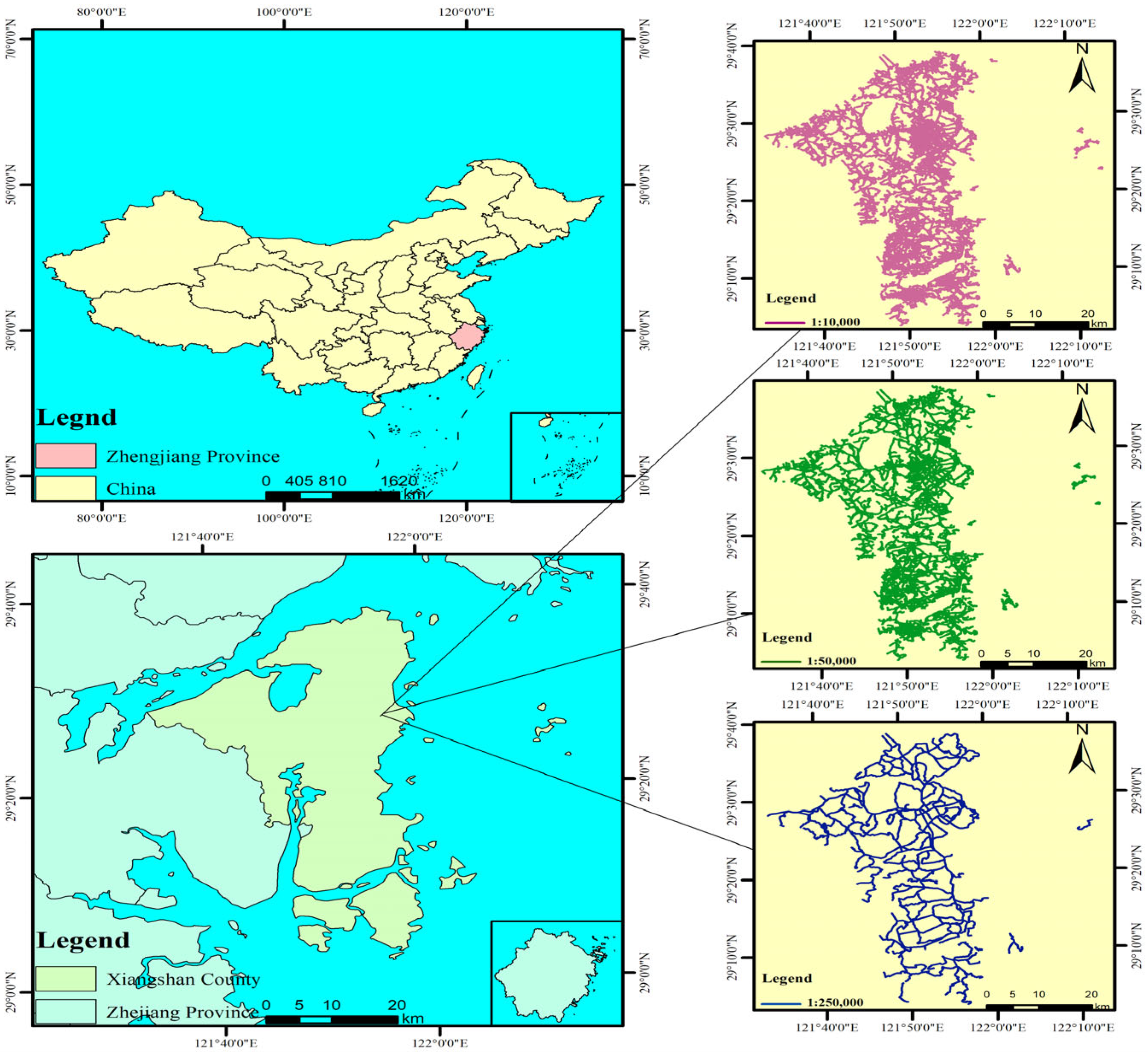
Considering that the span of the scales 1:10,000 and 1:250,000 is large and the accuracy of the experimental results is low, in this paper, the road dataset with scales 1:50,000 and 1:250,000 and the road data with scales 1:10,000 and 1:50,000 are respectively named as Group A and Group B for road-matching experiments. The road dataset with a scale of 1:250,000 is the reference road dataset in Group A, and the road dataset with a scale of 1:50,000 is the reference road dataset in Group B. In this paper, a total of seven road-matching models are selected to be applied in the matching of the experimental road dataset. Among them, length, direction, and Hausdorff distance are used as the common matching indices for these seven road datasets, while the ISOD descriptor, included angle chain, and camber variance are added to the road-matching models either individually or in combination. In this paper, the weight of each metric in each model is determined by controlling a single variable. When determining the weights for a particular model, the weights of one of the features are first changed; the weights of the other features are set and kept constant, and then, multiple comparison experiments are conducted. The weight corresponding to the indicator with the best matching result is the weight of that indicator in that model. Subsequently, the weight of the next indicator is changed; the weights of the other indicators are kept unchanged, and then, several comparison experiments are conducted to select the weight with the best matching result. By analogy, the weights of each indicator in the model can be determined to match those in groups A and B, respectively. The weights of each indicator in the seven models were normalized.

Table 6. Allocation of Index Weights for 7 Models in Group A Experiment.

Matching Models	Similarity Indicators
	Length	Directions	Hausdorff Distance	ISOD	Included Angle Chain	Camber Variance
Models I	0.2	0.2	0.85	0.8
Models Cr	0.2	0.2	0.95		0.7
Models Cv	0.2	0.3	0.8			0.3
Models ICr	0.1	0.2	0.9	0.8	0.7
Models ICv	0.1	0.1	0.9	0.9		0.1
Models CrCv	0.2	0.2	0.9		0.6	0.1
Models ICrCv	0.2	0.3	0.9	0.7	0.6	0.1

and

Table 7. Allocation of Index Weights for 7 Models in Group B Experiment.

Matching Models	Similarity Indicators
	Length	Directions	Hausdorff Distance	ISOD	Included Angle Chain	Camber Variance
Models I	0.3	0.25	0.9	0.9
Models Cr	0.3	0.3	0.75		0.65
Models Cv	0.35	0.4	0.7			0.2
Models ICr	0.2	0.3	0.85	0.8	0.75
Models ICv	0.3	0.3	0.8	0.75		0.2
Models CrCv	0.25	0.25	0.8		0.5	0.2
Models ICrCv	0.3	0.35	0.8	0.9	0.7	0.15

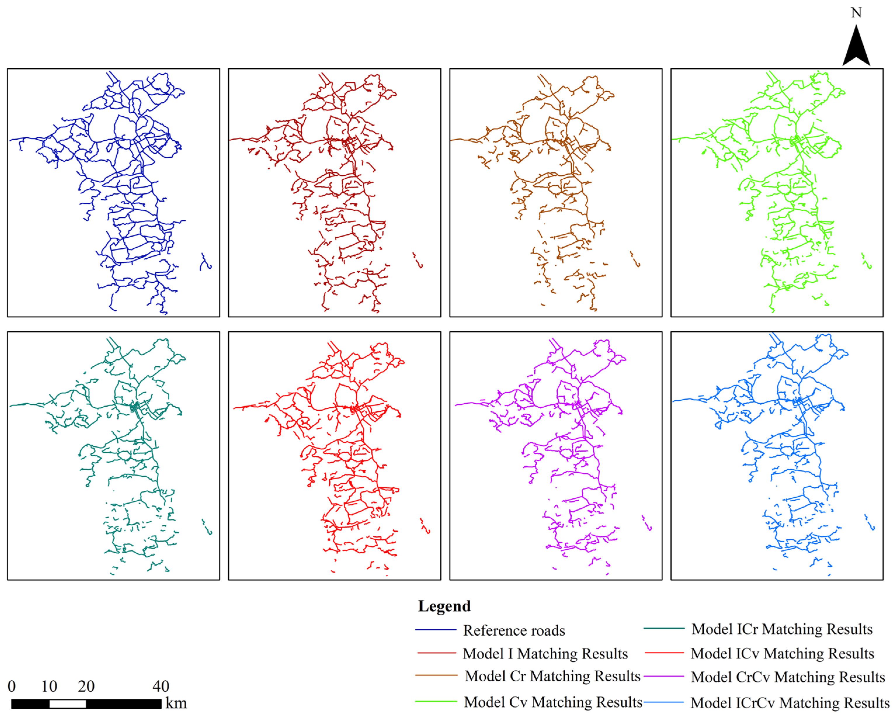
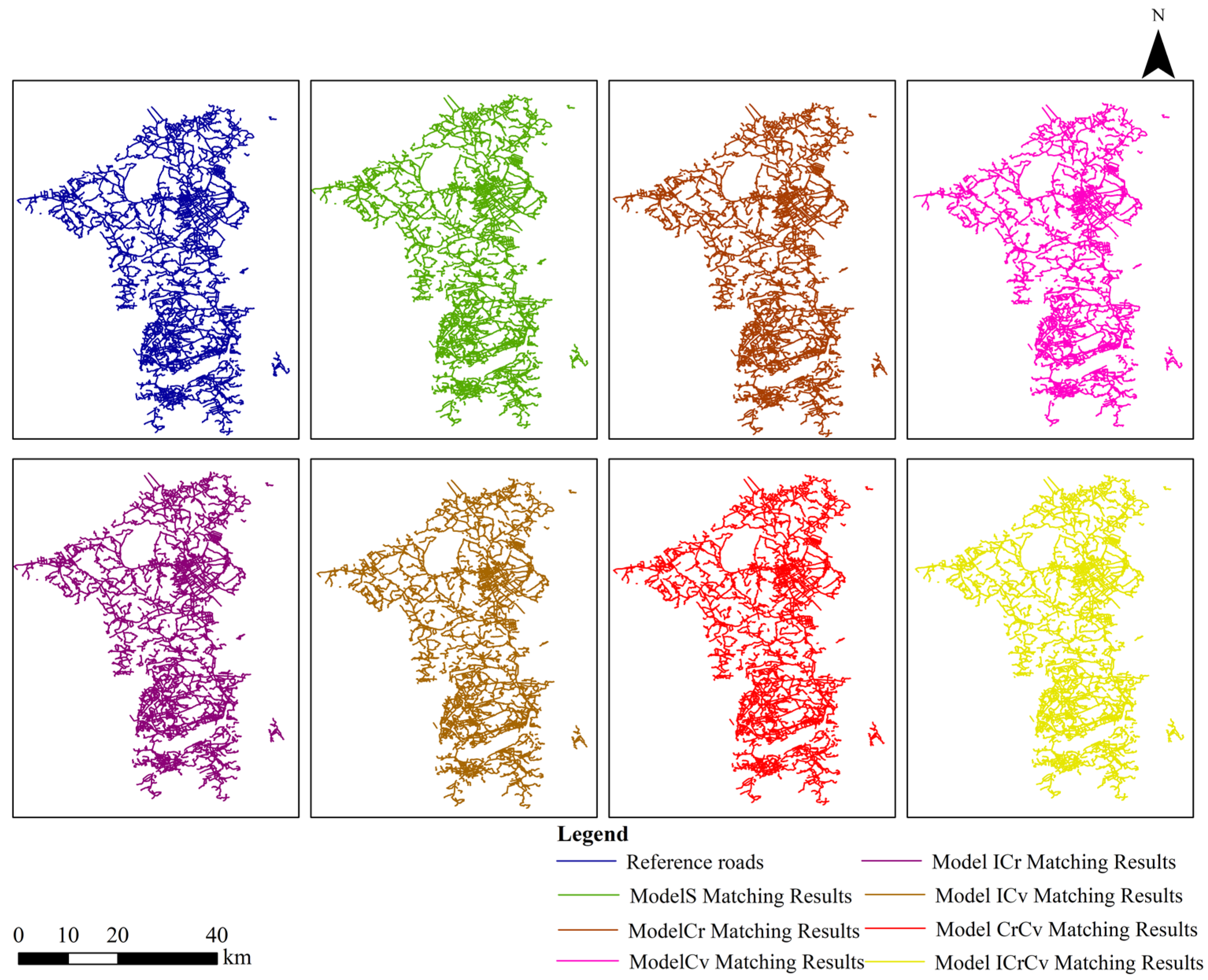
show the allocation of each metric for the seven models in the Group A and Group B experiments, respectively. The matching results were then output, as shown in Figure 9 and Figure 10. In Group A, the matching results can be directly compared with the original data, allowing for an intuitive assessment of the matching model’s performance. In contrast, the experimental data in Group B is more complex, making it difficult to clearly demonstrate the model’s performance through direct comparison. A detailed analysis and comparison of the relevant matching results will be presented step by step in the discussion section.

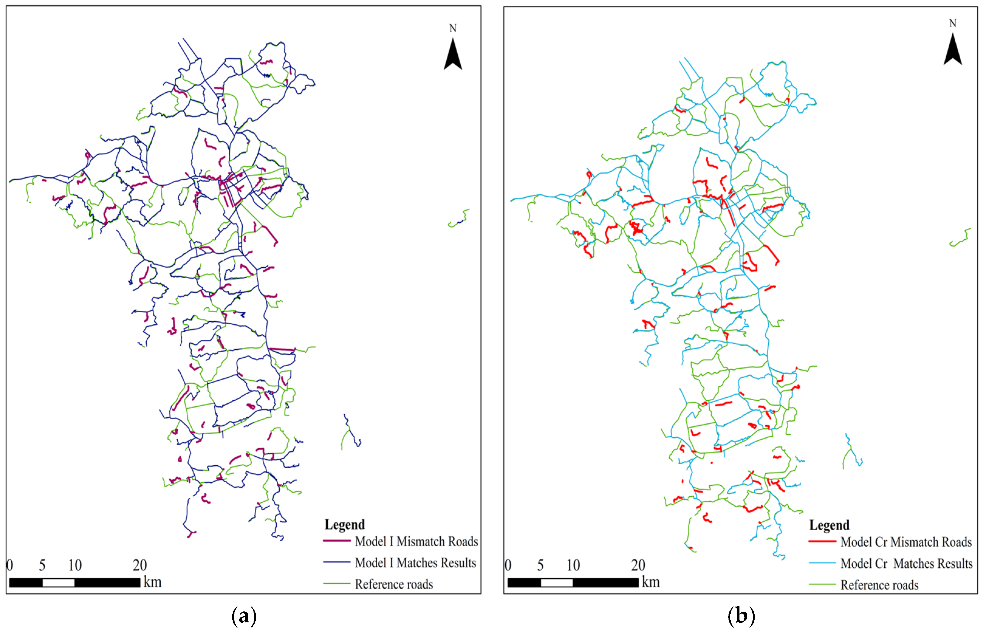
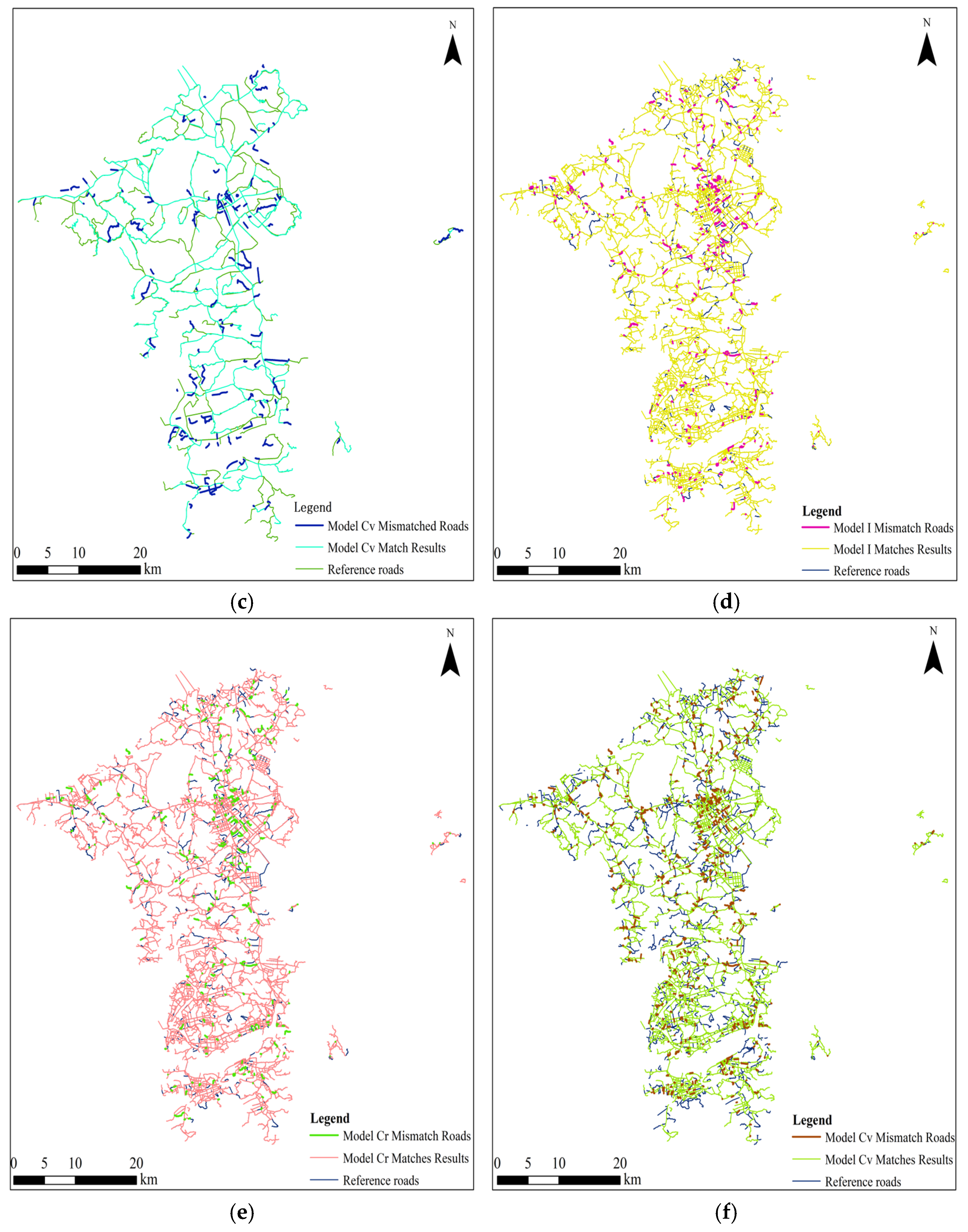
Firstly, this paper compares and analyzes the matching results of models I, Cr, and Cv. The similarity features shared by these three models are length, direction, and Hausdorff distance, and the differences are that the three models combine ISOD descriptors, included angle chain, and camber variance, respectively. The result output plots of the integrated metric models combining the four similarity features, as well as the data, were output (as shown in

Table 8. Evaluation results of Models I, Cr, and Cv in Experiment A.

Matching Models	Precision (%)	Recall (%)	F-Score Value (%)
Models I	86.39	94.06	90.06
Models Cr	85.15	89.55	89.29
Models Cv	76.60	91.25	83.29

and

Table 9. Evaluation results of Models I, Cr, and Cv in Experiment B.

Matching Models	Precision (%)	Recall (%)	F-Score Value (%)
Models I	94.75	93.34	94.04
Models Cr	95.20	92.98	94.08
Models Cv	86.48	86.46	86.47

, and Figure 11), and comparative analyzes were carried out by comparing the allocation of mismatched roads in the target roads as well as the evaluation metrics.

Based on the above results, the three features are analyzed from the perspective of how individual geometric features influence the outcomes.

Overall, in the matching experiments of Group A, under the condition that the three common indicators remain unchanged, the model I combined with the improved SOD achieves the highest F-score value, indicating the best matching performance. The reference dataset in Group A has a scale of 1:250,000, where most roads are main roads and only a few are branch roads. According to the result graphs, missed matches are primarily found on main roads, while incorrect matches are more frequently observed on branch roads. In the matching experiment of Group B, under the condition that the three indicators remain unchanged, the model Cr combined with the included angle chain achieves the highest F-score value, indicating the best matching performance. The reference dataset in Group B has a larger scale of 1:50,000, providing more detailed road representations. The distinction between trunk and branch roads is clearer. Missed matches are mainly distributed along branch roads, whereas incorrect matches are predominantly found on trunk roads. It can be seen that when matching small-scale road datasets, we can consider combining spatial relationship indicators based on geometric similarity indicators, i.e., ISOD descriptors, to match road datasets, and the matching effect is better. When matching between large-scale road datasets, the geometric similarity index can be considered to be combined with the included angle chain, and the matching effect is better.

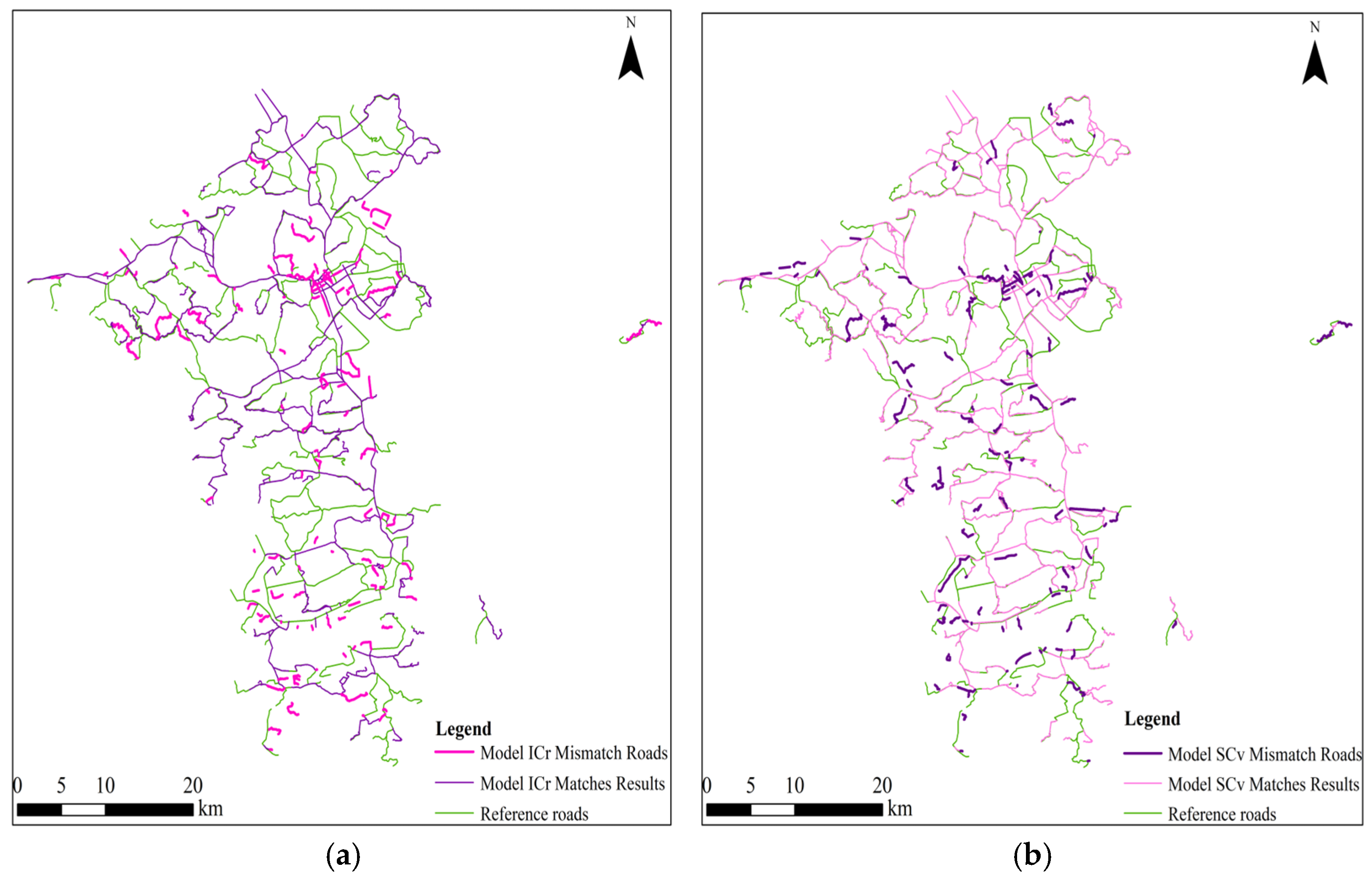
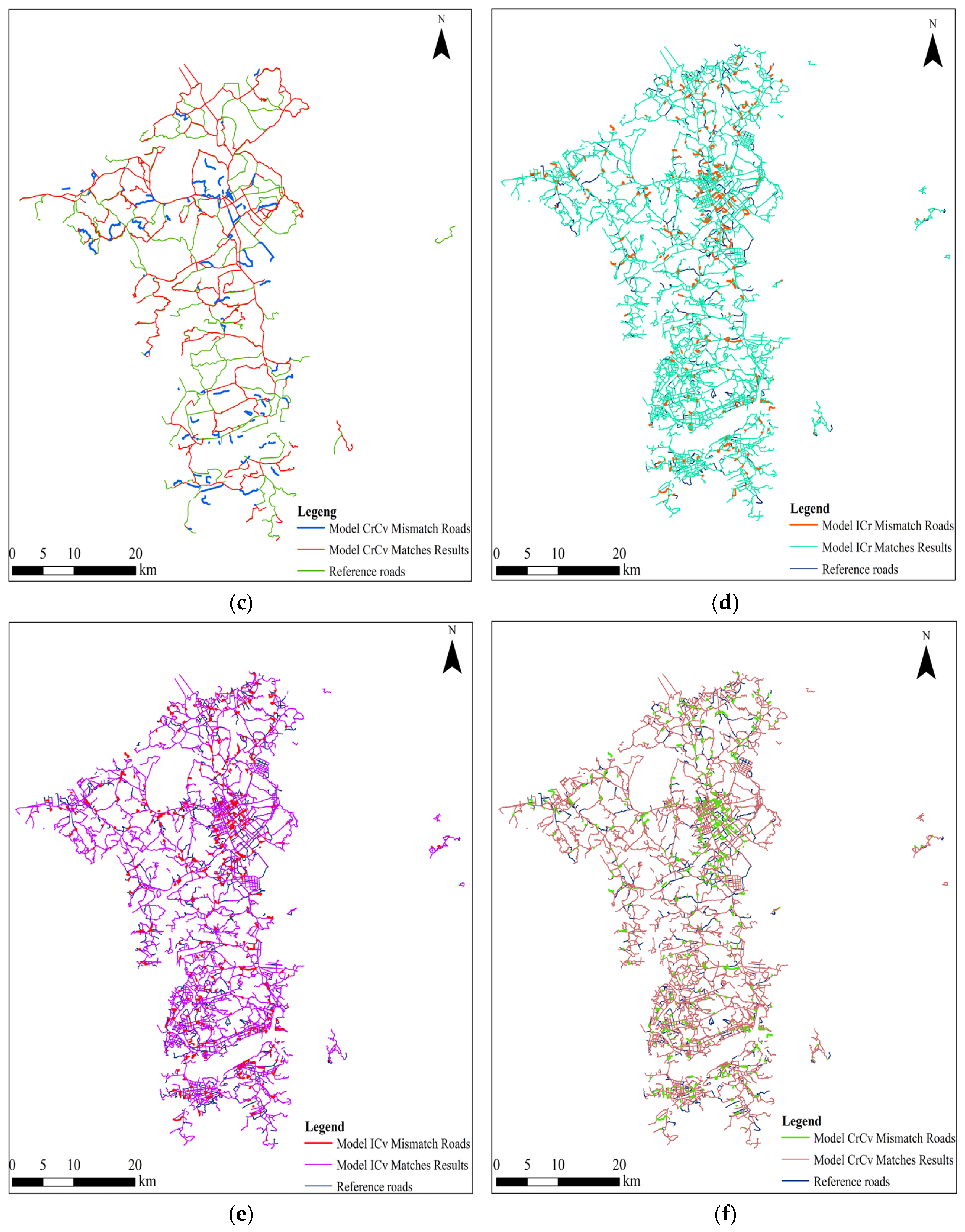
Subsequently, this paper outputs the output plots of the matching results of the integrated metric models ICr, ICv, and CrCv, which combine the five similarity features, as well as the data (as shown in

Table 10. Evaluation results of models ICr, ICv, and CrCv in Experiment A.

Matching Models	Precision (%)	Recall (%)	F-Score Value (%)
Models ICr	76.81	87.35	81.74
Models ICv	81.96	93.06	87.16
Models CrCv	82.73	89.48	85.97

and

Table 11. Evaluation results of models ICr, ICv, and CrCv in Experiment B.

Matching Models	Precision (%)	Recall (%)	F-Score Value (%)
Models ICr	94.91	93.06	93.98
Models ICv	88.86	88.76	88.81
Models CrCv	90.81	90.01	90.41

, and Figure 12), and performs comparative analyzes by comparing the allocation of the mismatched roads among the target roads, as well as evaluating the metrics.

From the perspective of geometric feature complementarity, the three indicators are analyzed in pairs to evaluate the matching capability of the models from multiple angles.

In the road dataset matching experiments of Group A, under the condition that the three common indicators remain unchanged, the model ICv, which combines ISOD descriptors and camber variance, achieves the highest F-score value, indicating the best matching performance. Mismatches are mainly distributed on trunk roads, while mismatches are more evenly distributed on trunk and branch roads, but are more concentrated in areas with dense branch roads. In the road dataset-matching experiments of Group B, the model ICr, which combines ISOD descriptors and the included angle chain, achieves the highest F-score value under the condition that the three common indicators remain unchanged, indicating the best matching performance. Mismatches are distributed in both main roads and branch roads, while incorrect matches are mainly distributed in branch roads.

When performing the matching of small-scale road datasets while keeping length, distance, and direction constant, the combination of the ISOD descriptor and camber variance can be considered for matching since it has the best matching effect. When matching large-scale road datasets, the ISOD descriptor and the included angle chain have the best matching effect. Spatial relationships can be used for the matching of both large-scale and small-scale road datasets since the matching effect is more accurate.

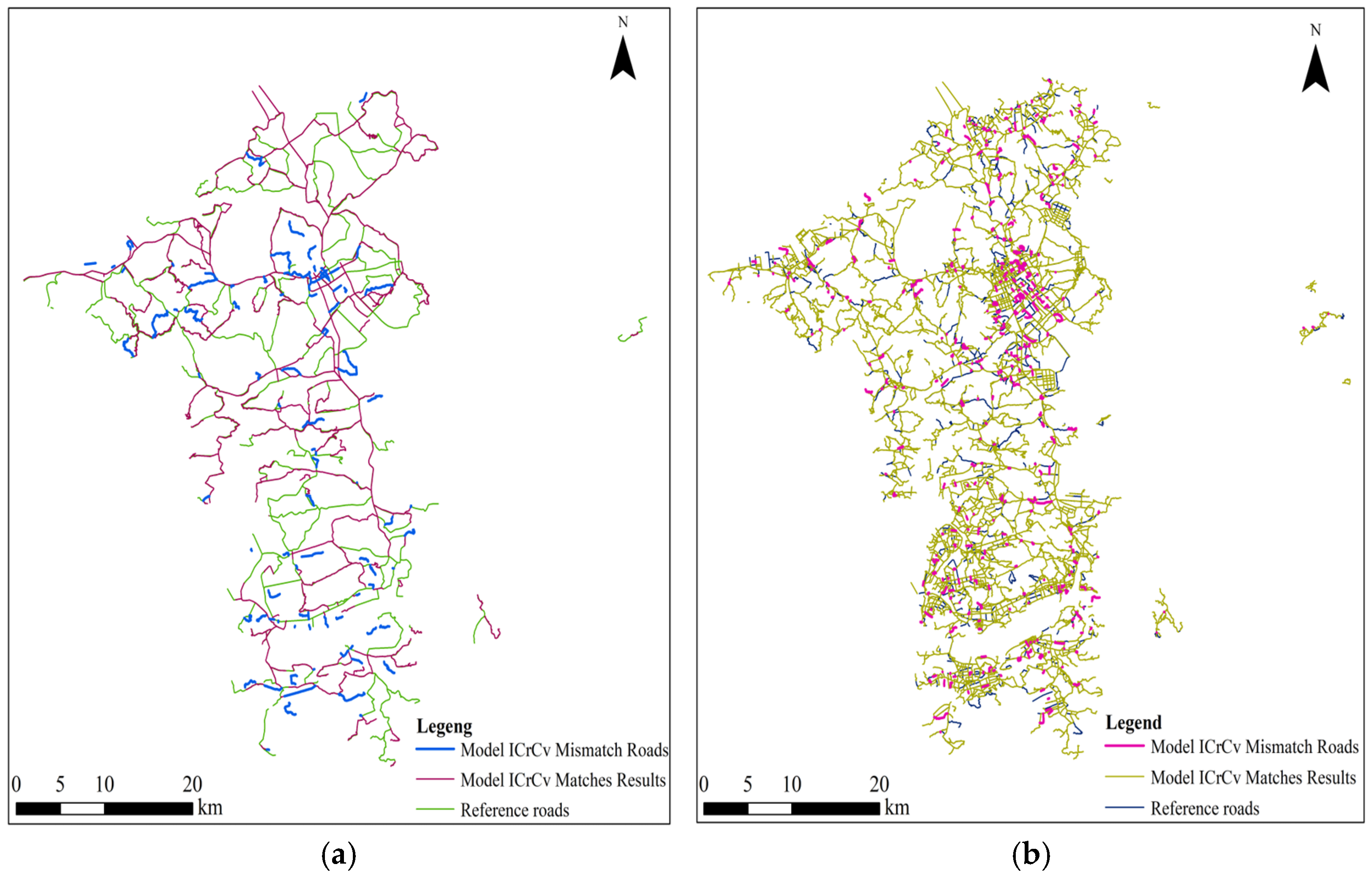
Subsequently, the matching results of the model ICrCv in Groups A and B experiments are compared and analyzed in this paper (as shown in

Table 12. Evaluation results of Model ICrCv in Experiment A.

Matching Models	Precision (%)	Recall (%)	F-Score Value (%)
Models ICrCv	83.57	90.17	86.74

and

Table 13. Evaluation results of Model ICrCv in Experiment B.

Matching Models	Precision (%)	Recall (%)	F-Score Value (%)
Models ICrCv	91.01	90.54	90.27

, and Figure 13). With the increase in similarity index, the matching model is more constrained for road-matching, and ISOD descriptors, included angle chain, and camber variance are added at the same time while keeping the distance, length, and direction unchanged. By comparing the matching results, this model is more suitable for road matching between large-scale road datasets. In Group A experiments, mismatching cases are distributed in the main roads, and incorrect matching cases are mainly distributed in the branch roads. In Group B experiments, the mismatches are mainly distributed in branch roads. Incorrect matches are distributed in both main roads and branch roads, and these matches are more concentrated in areas with dense branch roads.

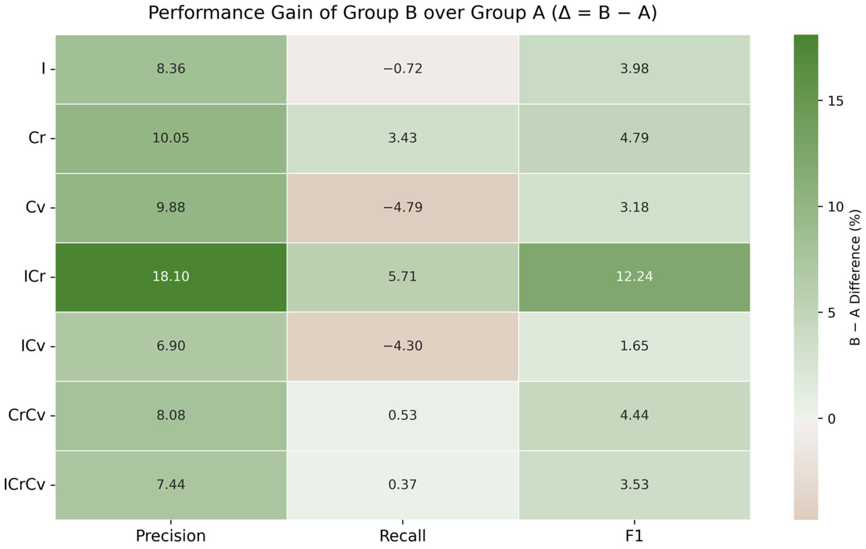
Ultimately, this study compares the matching results of the seven models in the two groups of road datasets and analyzes the matching results in terms of the precision, recall, and F-score values. The overall matching results for the road datasets in Groups A and B are shown in

Table 14. Matching results of Group A road dataset.

Matching Models	FN	FP	TP	Precision (%)	Recall (%)	F-Score (%)
Models I	69	172	1092	86.39	94.06	90.06
Models Cr	105	157	900	85.15	89.55	89.29
Models Cv	102	325	1064	76.60	91.25	83.29
Models ICr	129	269	891	76.81	87.35	81.74
Models ICv	83	245	1113	81.96	93.06	87.16
Models CrCv	107	190	910	82.73	89.48	85.97
Models ICrCv	102	184	936	83.57	90.17	86.74

and

Table 15. Matching results of Group B road dataset.

Matching Models	FN	FP	TP	Precision (%)	Recall (%)	F-Score (%)
Models I	582	452	8158	94.75	93.34	94.04
Models Cr	602	402	7971	95.20	92.98	94.08
Models Cv	1148	1146	7333	86.48	86.46	86.47
Models ICr	598	430	8021	94.91	93.06	93.98
Models ICv	965	955	7620	88.86	88.76	88.81
Models CrCv	843	769	7598	90.81	90.01	90.41
Models ICrCv	804	760	7695	91.01	90.54	90.27

.

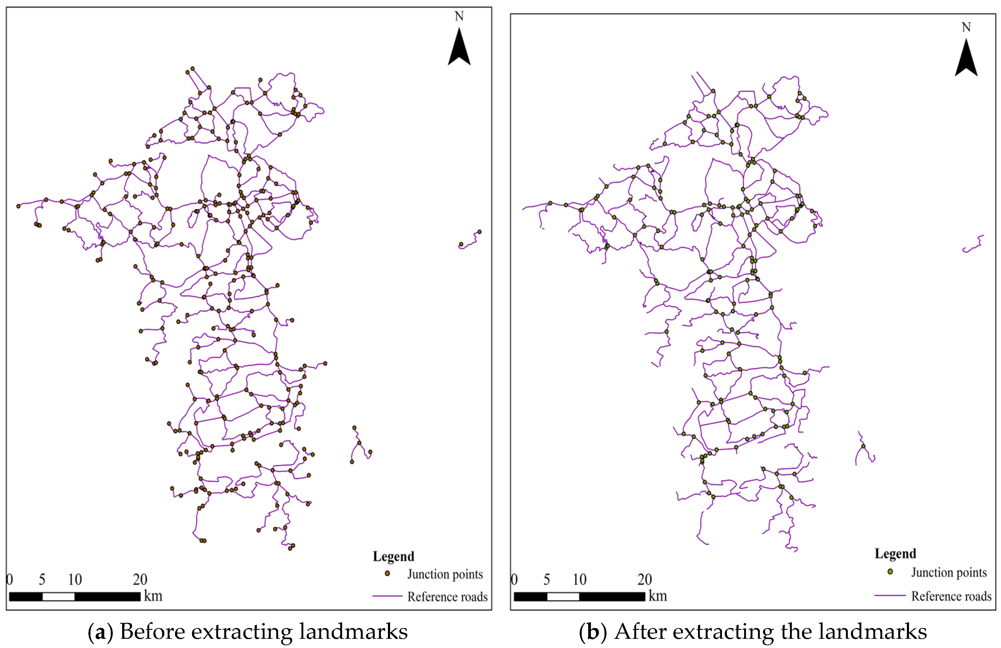
After multiple experimental verifications, we found that selecting the 20 nearest landmarks for each road segment can not only achieve a slight improvement in accuracy but also significantly enhance computational efficiency. As shown in

Table 16. Comparison of accuracy between SOD descriptor and ISOD descriptor.

Matching Models	A-F-Score (%)	F-Score Improvement (%)	B-F-Score (%)	F-Score Improvement (%)
Models I	90.06	4.61	94.04	3.5
Models S	85.45		91.54
Models ICr	81.74	1.69	93.98	2.51
Models SCr	80.05		91.47
Models ICv	87.16	1.99	88.81	2.63
Models SCv	85.17		86.24
Models ICrCv	86.74	1.51	90.27	3.26
Models SCrCv	85.23		87.06

and

Table 17. Comparison of time efficiency between SOD descriptor and ISOD descriptor.

Matching Models	A-Runtime (s)	Time Reduction (%)	B-Runtime (s)	Time Reduction (%)
Models I	1792.56	11.37	73,651.15	23.52
Models S	2022.47		96,303.52
Models ICr	1834.82	10.78	75,361.85	24.75
Models SCr	2056.44		100,153.55
Models ICv	1843.58	10.11	75,627.03	24.55
Models SCv	2051.02		100,234.25
Models ICrCv	1903.45	9.9	78,303.58	25.25
Models SCrCv	2112.01		104,754.05

, in large-scale datasets, the computational efficiency of the ISOD descriptor is improved by more than 20% compared with the SOD descriptor. Meanwhile, due to avoiding the interference of irrelevant landmarks, its accuracy has a more obvious improvement compared with small-scale datasets.

4. Discussion

As shown in Figure 14 and Figure 15, the comparative experimental results between Group A and Group B clearly reveal the key impact of scale differences on road network matching performance.

In Group A (matching 1:250,000 and 1:50,000 scales) with significant scale differences, the precision of each model shows a trend of first decreasing and then increasing, with the Cv model having the lowest precision and overall large fluctuations. This indicates that some descriptors (such as camber variance) are sensitive to the loss of geometric information caused by scale compression. In contrast, recall remains stable at around 90%, suggesting that despite certain mismatches, the models can still identify most true matching pairs. Notably, in Group A, the precision of all models is lower than recall, which is closely related to the reduced discriminative ability of the models due to excessive simplification of road features and blurred geometric information after scale compression. Model I achieves the highest precision and recall in this group, demonstrating its robustness in scenarios with significant scale differences.

In Group B (matching 1:10,000 and 1:50,000 scales) with smaller scale differences, the precision of all models is higher than recall, with small differences between the two, and the overall performance is more stable. This benefits from the complete preservation of road geometric features when scale consistency is high, making it easier for the models to achieve accurate matching. Model Cr obtains the highest precision, while Model I maintains the highest recall, reflecting good generalization ability and robustness.

The comparison of F-score further verifies the impact of scale differences: the overall F-score of Group A is lower than that of Group B, indicating that large-scale differences will weaken the integrity of road structure features and reduce the accuracy and consistency of matching.

In terms of the independent performance of each indicator, the performance when using camber variance alone is significantly inferior to that of other indicators, indicating that its ability to describe cross-scale features is rather limited. As shown in Table 16 and Table 17, the proposed ISOD descriptor exhibits strong adaptability under different scales. Particularly in Group A, its F-score is 4.61% higher than that of the original SOD, which proves that it can effectively retain multi-scale structural features and has strong anti-simplification ability. In addition, ISOD is significantly superior to SOD in both accuracy and time efficiency: when used alone, the accuracy is improved by 4.61%, and there is also a slight gain when combined with other indicators; in terms of time efficiency, it is improved by about 10% for small-scale data and more than 20% for large-scale data. Moreover, as the data scale increases, the efficiency advantage becomes more prominent, verifying its practicality and scalability in real applications.

5. Conclusions

With the rapid development of society and the economy, various fields are increasingly implementing higher requirements for the quality and availability of road data. As an important part of geospatial information, the accuracy and real-time performance of road data are crucial for urban planning, traffic management, disaster emergency response, and other fields. In this experiment, we first introduced the ISOD descriptor, which outperforms the SOD descriptor in both accuracy and time efficiency. Subsequently, based on three similarity features—length, Hausdorff distance, and direction—we constructed a comprehensive similarity measurement model for multi-scale road-matching experiments. This model incorporates the ISOD descriptor, included angle chain, and camber variance to handle map scales of 1:10,000 vs. 1:50,000 and 1:50,000 vs. 1:250,000. By comparing the results of the experiments, it is found that the matching effect on the large-scale road network is better than that of the small-scale road network matching as a whole, which is because the large-scale road network has more detailed and precise road information and provides more road-matching points. In the same set of experiments, with the change in the number of model indicators, the overall matching effect will also change since the model needs to consider changes in information complexity. The experiments found that the comprehensive similarity metric model constructed through multiple indicators can more accurately reflect the actual characteristics of the road to improve matching accuracy. Due to the complexity and diversity of road data sources, the use of integrated evaluation models reduces the reliance on a single indicator, improves robustness, and is more adaptable to different environments.

This experiment is based on three geometric features and innovatively integrates three descriptors—the ISOD descriptor, included angle chain, and camber variance—to construct a fusion model with several different descriptors, enriching the comprehensive similarity metric modeling approach in the field of multi-scale road matching. However, there are also shortcomings in this experiment. Although two new descriptors are introduced, the complexity of the matching process increases along with the increase in the number of model features, which reduces the efficiency of matching. In addition to this, the selection of metrics for evaluating this model is a challenge. How to effectively fuse the information of different features and the different matching methods may have a significant impact on the results.

References

1. Zhang, J.; Wang, Y.; Zhao, W. An improved probabilistic relaxation method for matching multi-scale road networks. Int. J. Digit. Earth 2018, 11, 635–655. [Google Scholar] [CrossRef]
2. Wan, B.; Yang, L.; Zhou, S.; Wang, R.; Wang, D.; Zhen, W. A Parallel-Computing Approach for Vector Road-Network Matching Using GPU Architecture. ISPRS Int. J. Geo-Inf. 2018, 7, 472. [Google Scholar] [CrossRef]
3. Chehreghan, A.; Ali Abbaspour, R. An assessment of the efficiency of spatial distances in linear object matching on multi-scale, multi-source maps. Int. J. Image Data Fusion 2018, 9, 95–114. [Google Scholar] [CrossRef]
4. Lewandowicz, E.; Flisek, P. A Method for Generating the Centerline of an Elongated Polygon on the Example of a Watercourse. ISPRS Int. J. Geo-Inf. 2020, 9, 304. [Google Scholar] [CrossRef]
5. Zhao, L.; Liu, Y.; Lu, Y.; Sun, Y.; Li, J.; Yao, K. Research on Vector Road Data Matching Method Based on Deep Learning. J. Appl. Math. Phys. 2013, 11, 303–315. [Google Scholar] [CrossRef]
6. Li, W.; Wang, Y.; Li, D.; Xu, X. MCM: A Robust Map Matching Method by Tracking Multiple Road Candidates. In Proceedings of the International Conference on Algorithmic Applications in Management, Guangzhou, China, 13–14 August 2022; pp. 231–243. [Google Scholar]
7. Zhang, Z. Spatial Data Orgnization of Multi-Scale Linear Objects Based on Features. Master’s Thesis, Wuhan University, Wuhan, China, 2005. [Google Scholar]
8. Singh, S.; Singh, J.; Goyal, S.; EI Barachi, M.; Kumar, M. Analytical Review of Map Matching Algorithms: Analyzing the Performance and Efficiency Using Road Dataset of the Indian Subcontinent. Arch. Arch. Comput. Methods Eng. 2023, 30, 4897–4916. [Google Scholar] [CrossRef]
9. Ma, S.; Lee, H. A Practical HMM-Based Map-Matching Method for Pedestrian Navigation. In Proceedings of the International Conference on Information Networking (ICOIN), Bangkok, Thailand, 11–14 January 2023; pp. 806–811. [Google Scholar]
10. Xu, F.; Deng, M.; Zhao, B.; Chen, J. A detailed investigation on the methods of object matching. J. Geo-Inf. Sci. 2009, 11, 657–663. [Google Scholar] [CrossRef]
11. Zhao, B. A Study on Multi-Scale Vector Map Objects Matching Method and Its Application. Ph.D. Thesis, Central South University, Changsha, China, 2011. [Google Scholar]
12. Wu, Z.; Xie, J.; Wang, Y.; Nie, Y. Map matching based on multi-layer road index. Transp. Res. Part C Emerg. Technol. 2020, 118, 102651. [Google Scholar] [CrossRef]
13. Walter, V.; Fritsch, D. Matching spatial data sets: A statistical approach. Int. J. Geogr. Inf. Sci. 1999, 13, 445–473. [Google Scholar] [CrossRef]
14. Fiset, R.; Cavayas, F.; Mouchot, M.; Solaiman, B.; Desjardins, R. Map-image matching using a multi-layer perceptron: The case of the road network. ISPRS J. Photogramm. Remote Sens. 1998, 53, 76–84. [Google Scholar] [CrossRef]
15. Abdolmajidi, E.; Mansourian, A.; Will, J.; Harrie, L. Matching authority and VGI road networks using an extended node-based matching algorithm. Geo-Spat. Inf. Sci. 2015, 18, 65–80. [Google Scholar] [CrossRef]
16. Chen, J.; Qian, H.; Wang, X.; He, H.; Hu, H. Improving the Matching Rate of Line Feature by Using Dynamic Simplification. Acta Geod. Cartogr. Sin. 2016, 45, 486–493. [Google Scholar]
17. Kim, J.; Yu, K.; Heo, J.; Lee, W. A new method for matching objects in two different geospatial datasets based on the geographic context. Comput. Geosci. 2010, 36, 1115–1122. [Google Scholar] [CrossRef]
18. Zhong, D. Research on Line Features Quality Assessment and Multi-Scale Water System Matching Method. Master’s Thesis, Wuhan University, Wuhan, China, 2018. [Google Scholar]
19. Lai, Y.; Sun, D.; Liao, X.; Sun, H. Algorithm of map-matching based on road buffer analysis. Appl. Res. Comput. 2011, 28, 3312–3314. [Google Scholar]
20. Wu, H.; Xu, S.; Huang, S.; Wang, J.; Yang, X.; Liu, C.; Zhang, Y. Optimal road matching by relaxation to min-cost network flow. Int. J. Appl. Earth Obs. Geoinf. 2022, 114, 103057. [Google Scholar] [CrossRef]
21. Zhang, Y.; Yang, B.; Luan, X. Automated Matching Urban Road Networks Using Probabilistic Relaxation. Acta Geod. Cartogr. Sin. 2012, 41, 933–939. [Google Scholar]
22. Chehreghan, A.; Ali Abbaspour, R. A geometric-based approach for road matching on multi-scale datasets using a genetic algorithm. Cartogr. Geogr. Inf. Sci. 2018, 45, 255–269. [Google Scholar] [CrossRef]
23. Zhuang, Q. Research on Road Network Matching Method Based on Knowledge Graph. Master’s Thesis, Henan University, Zhengzhou, China, 2024. [Google Scholar]
24. Fang, C.; Zhang, S. A Concept Semantic Similarity Method for Underground Pipeline Spatial Data Matching. J. Comput.-Aided Des. Comput. Graph. 2017, 29, 720–727. [Google Scholar]
25. Guo, W.; Liu, H.; Sun, Q.; Yu, A.; Ding, Z. A multisource contour matching method considering the similarity of geometric features. Acta Geodaetica Cartogr. Sin. 2019, 48, 643–653. [Google Scholar]
26. Kim, I.; Feng, C.; Wang, Y. A simplified linear feature matching method using decision tree analysis, weighted linear directional mean, and topological relationships. Int. J. Geogr. Inf. Sci. 2017, 31, 1042–1060. [Google Scholar] [CrossRef]
27. Zhang, M.; Meng, L.; Bobrich, J. A road-network matching approach guided by ‘structure’. Ann. GIS 2010, 16, 165–176. [Google Scholar] [CrossRef]
28. Chehreghan, A.; Ali Abbaspour, R. A new descriptor for improving geometric-based matching of linear objects on multi-scale datasets. GIScience Remote Sens. 2017, 54, 836–861. [Google Scholar] [CrossRef]
29. Wang, P. Road Network Matching Based on Stable Hierarchical Spatial Morphology. Ph.D. Thesis, China University of Geosciences, Wuhan, China, 2017. [Google Scholar]
30. Hacar, M.; Gökgöz, T. A New, Score-Based Multi-Stage Matching Approach for Road Network Conflation in Different Road Patterns. ISPRS Int. J. Geo-Inf. 2019, 8, 81. [Google Scholar] [CrossRef]
31. An, X.; Sun, Q.; Wei, B. Feature Matching from Network Data at Different Scales Based on Similarity Measure. Geomat. Inf. Sci. Wuhan Univ. 2012, 37, 224–228+241. [Google Scholar]
32. Cai, H.; Mao, Y.; Zhu, X.; Fu, Y.; Zhou, R. Comparison of the Minimum Bounding Rectangle and Minimum Circumscribed Ellipse of Rain Cells from TRMM. Adv. Atmos. Sci. 2024, 41, 391–406. [Google Scholar] [CrossRef]
33. Yang, H.; He, Z.; Chen, H.; Zhou, Z.; Fan, Y. A Method for Automatic Generalization of Urban Settlements Considering Road Network. Geomat. Inf. Sci. Wuhan Univ. 2018, 43, 965–970. [Google Scholar]
34. Lu, Y.; Zhang, K.; Liu, S.; Wu, Y.; Zhao, G.; Li, Q.; Feng, C. A vector data matching algorithm based on slope difference and azimuth. J. Shandong Univ. (Eng. Sci.) 2016, 46, 31–39. [Google Scholar]
35. Zhao, D.; Hua, S. Research on Automatic Matching of Vector Road Networks Based on Global Optimization. Acta Geod. Cartogr. Sin. 2010, 39, 416–421. [Google Scholar]
36. Lu, Y. Research on Registration Method between Vector Data and Image Data Based on Shape Feature. Acta Geod. Cartogr. Sin. 2014, 43, 879. [Google Scholar]
37. Sun, Y.; Lu, Y.; Ding, Z.; Wen, Q.; Li, J.; Liu, Y.; Yao, K. Multi-Scale Road Matching Based on the Summation Product of Orientation and Distance and Shape Descriptors. ISPRS Int. J. Geo-Inf. 2023, 12, 457. [Google Scholar] [CrossRef]
38. Zhao, Y.; Chen, Y. Included Angle Chain: A Method for Curve Representation. J. Softw. 2004, 02, 300–307. [Google Scholar]
39. Haynes, R.; Jones, A.; Kennedy, V.; Harvey, I.; Jewell, T. District Variations in Road Curvature in England and Wales and their Association with Road-Traffic Crashes. Environ. Plan. A Econ. Space 2007, 39, 1222–1237. [Google Scholar] [CrossRef]
40. Wen, Q. Research on Multi-Scale Road Network Vector Data Matching Method. Master’s Thesis, Shandong University of Technology, Zibo, China, 2021. [Google Scholar]
41. Deng, M.; Li, Z.; Chen, X. Extended Hausdorff distance for spacial objects in GIS. Int. J. Geogr. Inf. Sci. 2007, 21, 459–475. [Google Scholar]
42. Deng, M.; Li, Z. A statistical model for direction relations between spacial objects. GeoInformatica 2008, 12, 193–217. [Google Scholar] [CrossRef]
Figure 1. Data of Road Networks at Different Scales in Xiangshan County, Zhejiang Province, China.
Ijgi 14 00280 g001
Figure 2. Schematic diagram of SOD descriptor sub-direction and distance.
Ijgi 14 00280 g002
Figure 3. Determine the starting point of the first line segment on an open curve. (a) Select the start point of the open curve once. (b) Select the start point of the open curve multiple times.
Ijgi 14 00280 g003
Figure 4. Determine the starting point of the first line segment on a closed curve.
Ijgi 14 00280 g004
Figure 5. Curve represented by included angle chain. (a) The curve represented when n = 6. (b) The curve represented when n = 8.
Ijgi 14 00280 g005
Figure 6. Multi-scale matching experiment flowchart.
Ijgi 14 00280 g006
Figure 7. Changes in the number of intersections before and after extracting landmarks from a 1:250,000 road dataset.
Ijgi 14 00280 g007
Figure 8. Changes in the number of intersections before and after extracting landmarks from a 1:50,000 scale road dataset.
Ijgi 14 00280 g008
Figure 9. Reference roads and experimental results of 7 models in Group A.
Ijgi 14 00280 g009
Figure 10. Reference roads and experimental results of 7 models in Group B.
Ijgi 14 00280 g010
Figure 11. Comparison of Matching Results of Models I, Cr, and Cv in Groups A and B. (a) Overlay of Model I matching results with 1:250,000 reference roads. (b) Overlay of model Cr matching results with 1:250,000 reference roads. (c) Overlay of model Cv matching results with 1:250,000 reference roads. (d) Overlay of Model I matching results with 1:50,000 reference roads. (e) Overlay of model Cr matching results with 1:50,000 reference roads. (f) Overlay of model Cv matching results with 1:50,000 reference roads.
Ijgi 14 00280 g011aIjgi 14 00280 g011b
Figure 12. The Comparison of matching results of models ICr, ICv, and CrCv in groups A and B. (a) Overlay of model ICr matching results with 1:250,000 reference roads. (b) Overlay of model ICv matching results with 1:250,000 reference roads. (c) Overlay of model CrCv matching results with 1:250,000 reference roads. (d) Overlay of model ICr matching results with 1:50,000 reference roads. (e) Overlay of model ICv matching results with 1:50,000 reference roads. (f) Overlay of model CrCv matching results with 1:50,000 reference roads.
Ijgi 14 00280 g012aIjgi 14 00280 g012b
Figure 13. Mismatched road Comparison of model ICrCv on target datasets of 1:50,000 and 1:10,000. (a) Overlay of model ICrCv matching results with 1:250,000 reference roads. (b) Overlay of model ICrCv matching results with 1:50,000 reference roads.
Ijgi 14 00280 g013
Figure 14. Comparison of evaluation indicators between Group A and Group B.
Ijgi 14 00280 g014
Figure 15. Comparison of the differences in evaluation indicators between Group A and Group B.
Ijgi 14 00280 g015