1. Introduction
For a long time, the study of the impact of the built environment on residents’ travel behavior has been a key topic in the field of transportation research [
1]. With the rapid acceleration of urbanization in China, the significant expansion of urban areas, and the large-scale construction of transportation infrastructure, the built environment has undergone dramatic changes. At the same time, accompanied by rapid socioeconomic development, residents’ travel behavior has become more diverse. In this context, the impact of the built environment on residents’ travel behavior is undergoing profound changes. Among them, the metro, as a special type of built environment, exerts dynamic impacts on the surrounding environment during its construction, and these effects indirectly influence residents’ travel behavior. Therefore, accurately assessing the impact of metro projects is crucial [
2].
It is worth noting that the subway has multiple attributes simultaneously; it can function as a built environment, like a Transit-Oriented Development (TOD) community. It can also serve as a type of transportation facility, such as rail stations. Furthermore, it provides a means of transportation. Depending on its classification, the subway exerts distinct impacts: as a travel mode, it directly influences residents’ commuting patterns; as transportation infrastructure, it indirectly alters travel expenses by enhancing accessibility, thereby influencing residents’ travel decisions [
3]; and as a unique built environment, it transforms land use patterns, alters daily lifestyles, and ultimately affects individual travel behaviors [
4]. Nevertheless, the current research on the influence of subway on travel behavior focuses more on the single attribute of subway, neglecting to integrate all three key attributes of subway systems and their interrelationships. Consequently, findings on fundamental inquiries remain inconclusive, particularly regarding whether the subway effectively reduces reliance on car travel. This is because the central debate revolves around whether shifts in residents’ travel patterns induced by subway systems stem from alterations in the surrounding built environment due to subway construction or enhancements in transportation accessibility facilitated by the subway itself. Moreover, it questions whether the subway’s influence on the built environment subsequently affects individual mobility. Clarifying these underlying mechanisms is imperative.
Indeed, as a reliable and efficient mode of transportation, the subway has markedly reduced car ownership and usage rates while mitigating surface-level traffic congestion [
5,
6]. Li studied the impact of metro accessibility on the travel mode choices of the 1980s generation in Shanghai. The study found that improved metro accessibility contributes to reducing car ownership and increasing the likelihood of metro commuting, but there is no evidence to suggest that it has an impact on car usage [
7]. Based on two mobility survey datasets, IBRAEVA used an autoregressive method to study the impact of TOD on the travel share of cars and buses. The results show that TOD has a significant suppressive effect on car usage. When TOD is present at both ends of the trip, the car share in the origin–destination (OD) pair decreases even more [
8]. Nevertheless, when considering built environment attributes, the subway not only influences residents’ travel choices but also profoundly impacts their behaviors and lifestyles, thereby extending its influence across all facets of daily life [
9]. For instance, Yan discovered that while the construction of subways reshapes the urban spatial structure, it also tends to exacerbate the phenomenon of the separation of residence and work. This leads to a significant increase in the spatial scale of residents’ daily household activities [
10], resulting in a greater dependence on private cars for both individual commuting and daily family life, potentially further suppressing the use of public transportation [
11]. Chatman’s study also found similar results. After controlling for built environment variables, residents living near train stations tended to make longer motor vehicle trips [
12]. Hence, by solely focusing on the travel mode aspect of subways while overlooking their built environment influence, one might mistakenly perceive subway construction as fostering car dependency. In light of this, while investigating the influence of subway systems on residents’ behavior, certain scholars additionally accounted for built environment variables. They designated analogous urban zones as the control counterparts for subway routes, examining the effect on leisure walking frequency. Their findings indicate a notable and distinct correlation between subway presence and increased walking activity [
13]. Nonetheless, significant disparities persist between this comparable area and an actual subway corridor concerning spatial built environments and demographic structures. To address these methodological limitations, subsequent researchers confined their study to the same spatial scope—specifically, alongside the subway route. Subsequently, researchers conducted comparative analyses using two temporal phases—pre- and post-subway inauguration—to examine shifts in residents’ travel behaviors from the subway’s inception to its establishment. DAI analyzed cross-sectional survey data before and after the opening of the Singapore Circle Line and found that the opening of the Circle Line increased the proportion of rail transit usage while decreasing the proportion of private car usage. However, there was no significant impact on the proportion of bus usage or travel patterns [
14,
15]. This approach embodies greater scientific rigor and methodological soundness. The primary challenge lies in acquiring relevant data from both pre- and post-subway phases, while mitigating confounding variables like urban social and economic developments during these periods.
Furthermore, according to individual activity theory, travel is a behavior originating from individuals seeking to satisfy their needs and engage in social interactions. Hence, travel behavior is regarded as subordinate to activity planning [
16]. Consequently, the subway system exerts distinct effects on both individual travel patterns and overall activity levels. For example, some affluent and well-educated residents reside in proximity to subway stations due to the augmented amenities brought about by the subway’s inauguration. However, their choice of residence does not stem from the intention to utilize the subway for commuting purposes [
17]. And further, the decline in car usage may not solely be attributed to the introduction of the subway. Simultaneously, as a result of the incremental enhancement of amenities along the subway route, the lifestyle and commuting patterns of this demographic are likely to undergo substantial transformations compared to their pre-relocation norms. For instance, following relocation to the subway corridor, the concentrated placement of schools mitigated the initial imbalance between educational access and residential placement. Moreover, the profusion of commercial and corporate amenities transformed the routine of parental school commutes from a linear to a multifaceted network, thereby reshaping the traditional ‘home-to-school’ commuting patterns and lifestyle [
18]. On the other hand, as a type of infrastructure, the subway exhibits distinct impacts on its surrounding areas [
17,
19]. Nevertheless, the majority of extant studies confine their analyses to single geographic areas, thereby failing to capture these differential effects.
Finally, few studies have examined the impact of metro systems on residents’ behavior under different scenarios, with most of these studies being conducted in European and American countries. For example, Cao focused on the influence of the Minneapolis metro corridor on residents’ public transport usage [
20]. However, these countries have well-established metro systems and excellent urban designs, which differ significantly from the actual situation in many Chinese cities, most of which are in the early stages of developing rail transit. Therefore, the findings from these studies are not directly applicable to practical guidance in China. For this reason, this paper selects the representative “sparsely distributed metro city” of Kunming as the research object to explore the impact of the process of metro construction—going from no metro system to having one—on urban residents’ travel behavior.
In conclusion, underpinned by extensive big data and open-source datasets, and complemented by micro-behavioral survey data, this study categorizes spatially into two types: continuous corridors and discrete stations along subway lines, guided by the principles of scenario classification, stratification, and sub-scaling. The analysis employs nuclear density analysis and other methodologies to assess how subway openings influence the built environment within 0–500 m and 500–1000 m from stations and along corridors. Secondly, leveraging survey data on residents’ travel patterns pre- and post-subway inauguration, we apply the propensity score matching (PSM) method to mitigate the effects of non-subway variables across distinct time frames. Subsequently, we compare residents’ behavioral adaptations along the transit route in both scenarios—with and without the subway—to underscore its impact on daily routines and travel habits. Finally, we designate car travel choice and distance as travel-level variables, and travel time and activity duration as activity-level variables. Separate models are developed for each of these four variables, followed by an analysis of their paths and influential mechanisms to discern direct impacts attributable to the subway and indirect effects mediated by alterations in the built environment.
The paper is organized as follows:
Section 1 introduces the research question, reviews the relevant literature, and identifies the research gaps.
Section 2 presents the study area and data.
Section 3 outlines the research design and modeling methodology.
Section 4 analyzes the changes in the built environment and residents’ behavior characteristics before and after the opening of the subway.
Section 5 presents the empirical results.
Section 6 summarizes the findings and discusses the policy implications.
2. Study Area and Data
2.1. Study Area
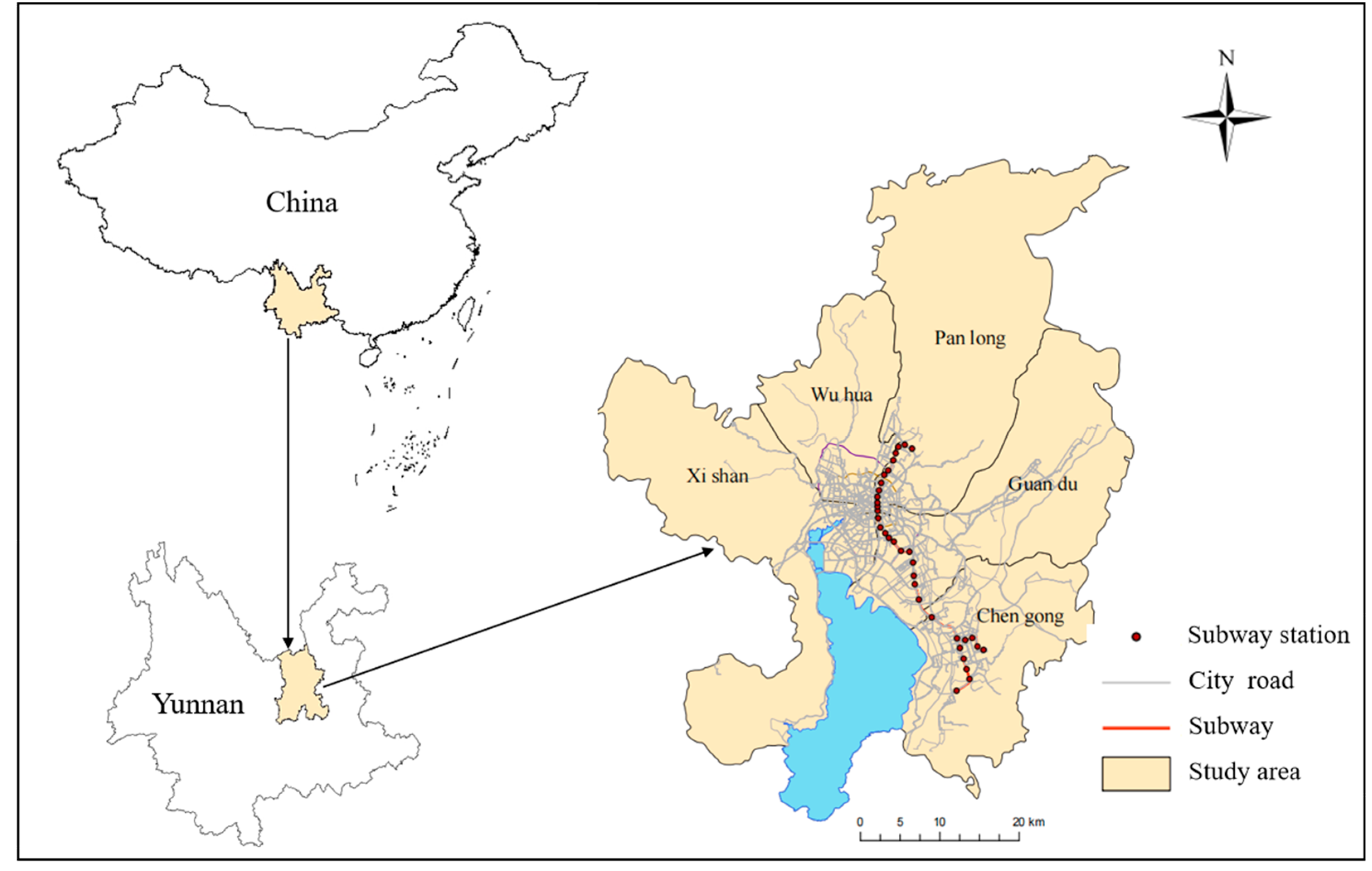
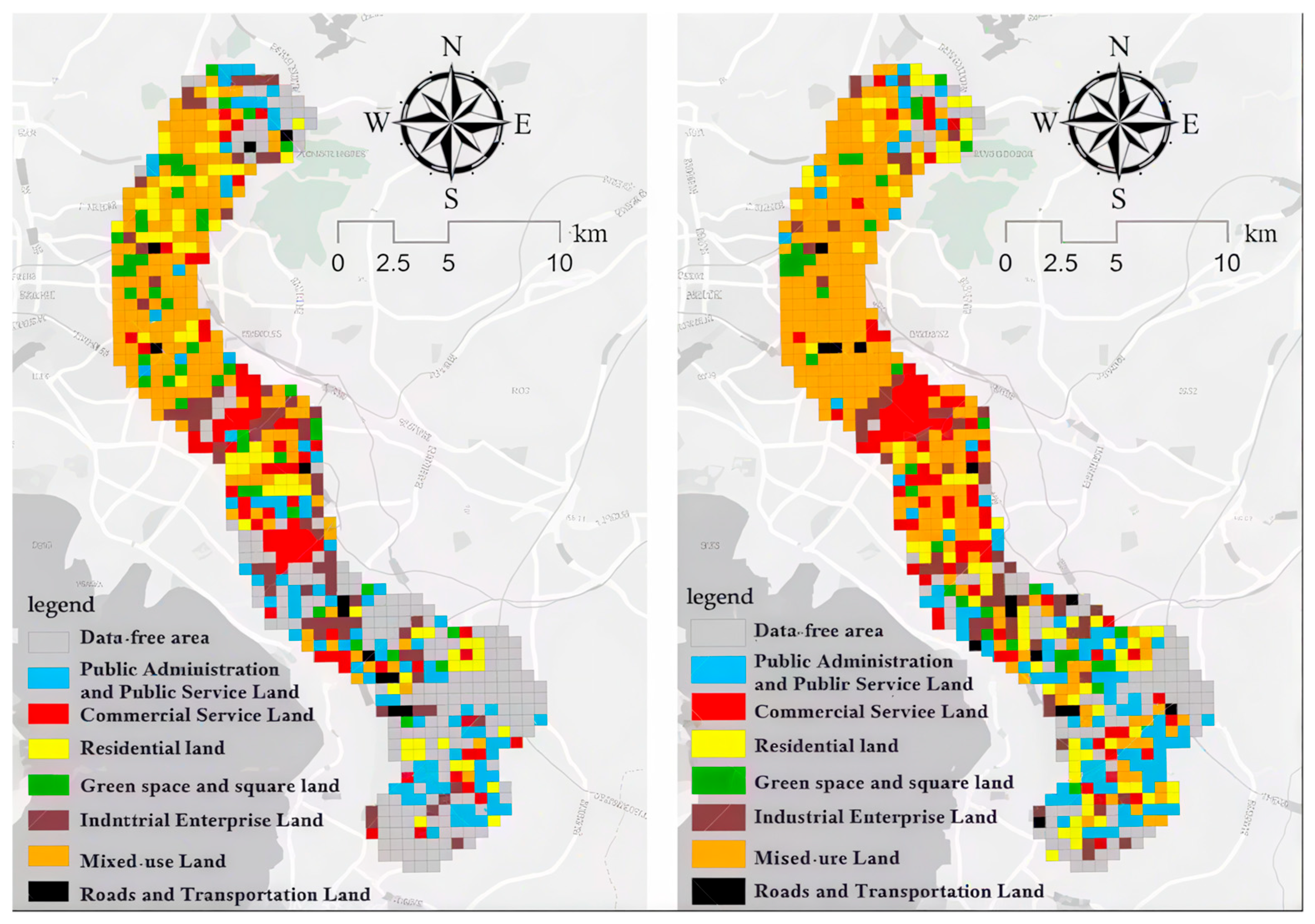
The data for this study is derived from the districts of Panlong, Guandu, Wuhua, Xishan, and Chenggong in Kunming City. Kunming, an important central city in Southwest China, is a typical monocentric city. For many years, the majority of the urban population, government administrative agencies, and public amenities were concentrated within the Second Ring Road of the old city, leading to progressively worsening traffic congestion. In response, government agencies, research institutions, and universities relocated to the southern New City area, prompting a significant influx of businesses and residents to Chenggong New Town. During this period, the urban land structure underwent substantial changes, with land development accelerating, and Chenggong New Town in the southern part of the city gradually expanding. However, large-scale infrastructure construction in the suburbs failed to effectively transform the traditional monocentric urban development model, instead exacerbating the job-housing separation in some areas. As a result, many residents began using private cars to commute between the main city and the new city. Meanwhile, the layout of the subway network and the expansion of transportation infrastructure were also incorporated into the city’s development agenda. Consequently, the transformation of the urban job-housing structure, driven by land development, and the large-scale construction of public transportation facilities have placed Kunming at a critical crossroads, where public transportation and private cars are in direct competition.
This research primarily focuses on Subway Lines 1 and 2, which comprise a total of 35 stations. These lines serve as vital transportation corridors in the city, characterized by high population density and discrepancies in urban development. Subway Line 6 is not included in the study due to its minimal influence on demographic and environmental factors. Refer to
Figure 1 for the geographical coverage.
2.2. Study Data
This study employed behavioral data from resident travel surveys conducted in Kunming in 2011 and 2016. The surveys were conducted prior to and following the inauguration of Kunming’s inaugural subway system, encompassing the city’s principal urban districts. In 2011, the survey involved participation from over 38,000 individuals across 20,643 households, resulting in 90,400 pieces of detailed travel data. In 2016, the survey included 32,664 households with over 80,000 residents, resulting in more than 183,000 travel records. The surveys collected socio-economic characteristics and travel patterns of respondents and their family members across the entire day.
In addition, we compared the basic social demographics, built environment, and public transportation information of Kunming City in 2011 and 2016, as shown in
Table 1. Over the five years, with the expansion of urban space and the widening of the urban framework, the activity space for residents has also increased. However, the development of basic service facilities has lagged behind, leading to an increase in travel distances for urban residents. The growth in per capita income and GDP has driven a rapid increase in the number of motor vehicles. At the same time, the accessibility of public transportation has also greatly improved, especially with the development of the subway (which went from non-existent to established). From 2016 to 2025, Kunming made significant progress in the development of urban rail transit. The metro network gradually improved, with the opening of Lines 4 and 5, forming an efficient transportation system with a “cross-shaped” structure as its backbone.
3. Methods
3.1. Research Design
The subway plays an important role in urban expansion and urban renewal. At the same time, the construction of the subway can influence people’s daily travel choices and their responses to the urban environment, indicating that the impact of the built environment on travel behavior changes with the emergence of the subway. Moreover, the subway has multiple attributes, and each of these attributes can have different levels of impact on the residents’ daily behaviors. Therefore, we hypothesize that the impact of the built environment on travel behavior will change during the process of the subway being established. By comparing modeling results from different periods, we aim to gain a deeper understanding of the long-term dynamic relationship between the subway, the built environment, and activity-based travel.
3.2. Variable Selection
The factors influencing residents’ travel and activities mainly come from three aspects: the built environment, residents’ socioeconomic attributes, and self-selection (attitude). First, existing research has shown that as population/employment density increases, the impact of built environment variables (such as population density) on travel behavior tends to weaken, and in some cases, may even reverse direction. Therefore, the influence of built environment factors (such as population density) on travel behavior may differ in the early stages of subway construction (when population density is low) compared to the later stages (when population density is high). Additionally, to eliminate the interference of confounding factors such as gender, household income, and education level, and to assess the true changes in residents’ travel and activities, we have controlled for the socioeconomic attributes of residents in the same strata across different years before modeling. The issue of self-selection has also been mitigated due to geographic location constraints, and the specific methods will be explained in the next section.
Correlations and collinearities among independent variables are examined after selecting indicators. After excluding variables with significant collinearity (VIF > 10), 9 built environment variables and 7 socioeconomic attributes were kept.
Table 2 shows the relevant variables. The diversity index, which measures land use mixing, is calculated using the formula
H is the mixing degree to be calculated; n is the category of POI; is the percentage of the number of Class i POIs in the total number of POIs.
The study analyzes changes in station infrastructure before and after subway inauguration using information entropy, dominance, and balance indices to assess diversity and equilibrium of station amenities. Information entropy measures diversity and complexity of local facilities, dominance and equilibrium indices evaluate evenness of facility distribution within a locale. Equations (1)–(3) present the formulas for these indices.
3.3. Propensity Score Matching
Before and after the subway opened, the social economy experienced rapid development, and the mobility of urban residents further increased. Whether during the construction or operation of the subway, it attracts groups who favor public transportation or are averse to the disturbances caused by traffic, leading to significant changes in the structural proportions of residents from various social strata within the research area, resulting in selection dilemmas. Therefore, simply dividing and conducting statistics based on spatial location may introduce certain biases in the final conclusions. To address this issue and eliminate the confounding effects of socioeconomic changes such as gender, household income, and educational level, we employed the Propensity Score Matching (PSM) method to control for temporal heterogeneity.
Propensity Score Matching (PSM) is a method used to address issues of data bias and confounding factors, commonly applied in fields such as econometric research. Its principle is based on the idea of matching estimators, using observable variables to match data from different groups. The main steps are as follows:
- (1)
ArcGIS (version 10.8.1) is a powerful geographic information system software used for map creation, spatial analysis, data management, and visualization. The buffer tool in ArcGIS is used to delineate two circular buffer zones, strictly based on Euclidean distance, namely 0–500 m and 500–1000 m, around the site. Based on these buffer zones, household, member, and travel information located in different ranges before and after the subway opening are extracted. The relevant information extracted is shown in
Table 3.
- (2)
The residents’ samples after the subway opened are classified as the treatment group, while the residents’ samples before the subway opened are classified as the control group. The samples after the subway opening are used to match the samples before the subway opening, which makes this matching method more aligned with actual conditions and results in minimal loss of useful information.
- (3)
A parallel trend test is conducted on the matching results of the treatment group and the control group, with the test results shown in
Table 4. From the table, it can be seen that the absolute value of the standardized bias after matching is within 10%, and the reduction in standardized bias is significant, while the
p-value after matching is not statistically significant. This indicates that the distribution of covariates between the treatment group and the control group is relatively balanced, and the matching is quite successful. After matching, the inner and outer circles obtained 1056 and 1405 pairs of resident samples, respectively.
3.4. Modeling Method Identification
The built environment data used in this study is considered aggregate data as it comes from the station area level, while socioeconomic attribute data is disaggregated, sourced from individual residents. To avoid ecological fallacy in modeling, the variability of dependent variables at the site level was evaluated. A two-level null model without explanatory variables was established using Equations (4) and (5), and the inter-group correlation coefficient (ICC) was used for assessment. If the ICC at the station level exceeded a certain threshold, a multi-level linear model (HLM) was used; otherwise, a traditional linear regression model (OLS) was employed.
Yij denotes the travel activity characteristics exhibited by the i-th resident at station j; βoj signifies the intercept at the individual level; βoj is considered as the random variable at the individual level; γoo represents the intercept derived from regression excluding station-specific considerations; μoj signifies the residual variance between the intercept of station j and the overall intercept.
Following the null model variance test, the results suggest that each dependent variable shows distinct site-level concentrations but generally displays weak overall associations. The academic community has yet to establish a clear critical value for ICC. For instance, Cohen proposed an ICC critical value of 0.059 [
21], James observed a median ICC value of 0.138 [
22], and Mathieu suggested using a cross-layer model when ICC falls between 0.15 and 0.30 [
23]. Based on these findings, a multiple linear regression model (OLS) was employed to analyze travel distance, travel time, and activity duration. The binary Logit model is used to study the impact of the built environment on travel behavior for car trips.
Multiple linear regression is a statistical method that combines two or more independent variables linearly to estimate or predict a dependent variable. The expression is as follows:
In the equation, represents the constant term; represents the regression coefficient; represents the n-th independent variable of individual i; represents the random error.
The binary Logit model is a type of generalized linear model where the dependent variable is a binary classification variable. It requires that the sum of the residuals is zero and follows a binomial distribution. Unlike linear models, this model uses the maximum likelihood method for estimation. The expression is as follows:
In the formula, is the constant term; is the regression coefficient; is the independent variable of the model.
5. Analysis of Influence on Residents’ Travel Activity Before and After Subway Opening
In the aforementioned feature analysis, the observed decrease in residents’ travel distances contradicts the anticipated expansion of residents’ activity spaces facilitated by subway infrastructure. The more substantial decline in the percentage of car journeys in the outer zones deviates from the anticipated influence of subway systems on automobile usage. Thus, travel distance and car travel will be scrutinized as variables influencing residents’ travel behaviors. Furthermore, residents’ time allocation is influenced by familial or personal factors, which operate distinctively from those impacting travel decisions. Accordingly, the consumption of travel time and the duration of activities, as variables influencing residents’ activities behaviors.
Linear regression models (OLSs) were constructed using the variables listed in
Table 2. The residuals of each model exhibited normal distribution, with a Durbin–Watson (DW) index close to 2, and the models passed the F-test. Therefore, we can confidently assert the validity of the model, given its adherence to the fundamental assumptions of linear regression. Subsequent analysis delves into the outcomes of these models.
5.1. Dependent Variable Is the Result of the Model of Car Travel Choice
Table 9 illustrates the impact of built environment and socioeconomic attributes on travel behavior in various scenarios and scales. Before the subway open, factors influenced car usage near the station. Limited parking in densely populated historic areas led residents to prefer non-car transport. Additionally, each extra family car increased the likelihood of car travel by 16 times. Conversely, in the outskirts, abundant recreational facilities reduced car dependency. Urban integration was found to increase car use, contrary to previous studies, possibly due to higher incomes and more car ownership in integrated areas, indirectly raising the likelihood of car travel.
Following the inauguration of the subway system, the proliferation of schools within the inner city area has notably fostered a heightened preference among residents for car-independent modes of transportation. This trend can be ascribed to diminished vehicular necessity facilitated by the close proximity and comprehensive accessibility of educational institutions. Concurrently, the seamless operation of the subway system affords residents the option to utilize it for their daily commutes, thereby mitigating reliance on automobiles. Despite car-owning households constituting the predominant demographic for vehicular travel, there has been a discernible rise in car usage subsequent to the subway’s commencement, relative to its pre-commencement period. In outlying areas, the proximity of bus stations significantly augments the accessibility of bus transit options, thereby diminishing residents’ dependency on personal vehicles to a certain degree.
5.2. The Model Results with the Dependent Variable Set as the Daily Travel Distance
Table 10 displays the model results, showing that before the subway opening, built environment variables affecting residents’ activity times in the inner circle are mainly related to density, while in the outer circle, they are influenced by both density and diversity. The inner circle model’s variables impacting travel distance changed pre and post subway opening, whereas the outer circle model’s variables showed consistent influence on travel distance.
Before the subway opening, the presence of schools and recreational facilities near the station increased travel distances, while the station population had the opposite effect. The reason is that the dense distribution of schools alleviates the unbalanced student-residence pattern and greatly reduces the travel distance of students and their companions. After the subway opened, the impact of school density on travel distances changed from negative to positive. This shift may be due to improved infrastructure near subway stations, changing residents’ commuting patterns. Before the subway, increased station integration in the outer circle led to longer travel distances due to enhanced infrastructure. Post-subway opening, substantial built environment factors within this region are expected to escalate.
5.3. The Model Result with the Dependent Variable Being the Duration of Activities Throughout the Day
Based on the model results (
Table 11), before the subway’s opening, the number of shopping facilities in the inner circle correlated positively with residents’ activity duration, while station population density showed a negative correlation. After the subway’s opening, there was a significant increase in factors affecting residents’ activity duration. The number of schools, station population density, and proximity to subway stations positively impacted activity duration, while population density had a negative correlation. Occupation had a significant influence on activity duration before the subway’s launch. After the inauguration, factors such as family size, income, and gender influenced activity duration, indicating changes in residents’ activity patterns due to subway construction. Before the subway’s opening, outer circle residents’ activity duration was influenced only by social and economic factors. After the opening, the built environment started to influence activity duration, with station population density and time savings from electric bicycle use showing positive correlations with activity duration.
6. Discussion and Conclusions
6.1. Discussion
This study explores the effects of the subway on residents’ travel behaviors and the relationship between the subway, built environment, and travel behavior. It examines changes in the built environment, residents’ characteristics, and behaviors before and after the subway’s introduction, guided by scenario analysis, hierarchical structuring, and scalar perspectives. The study has generated valuable research findings.
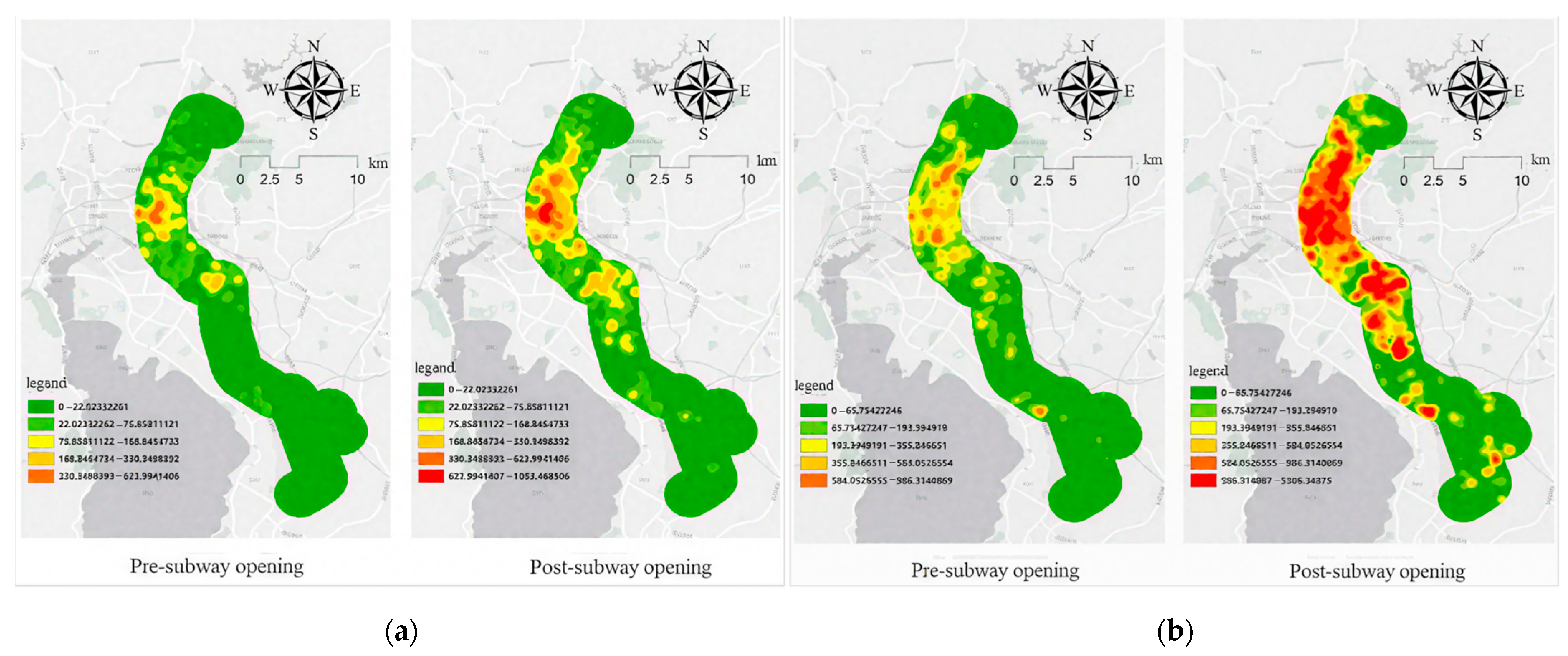
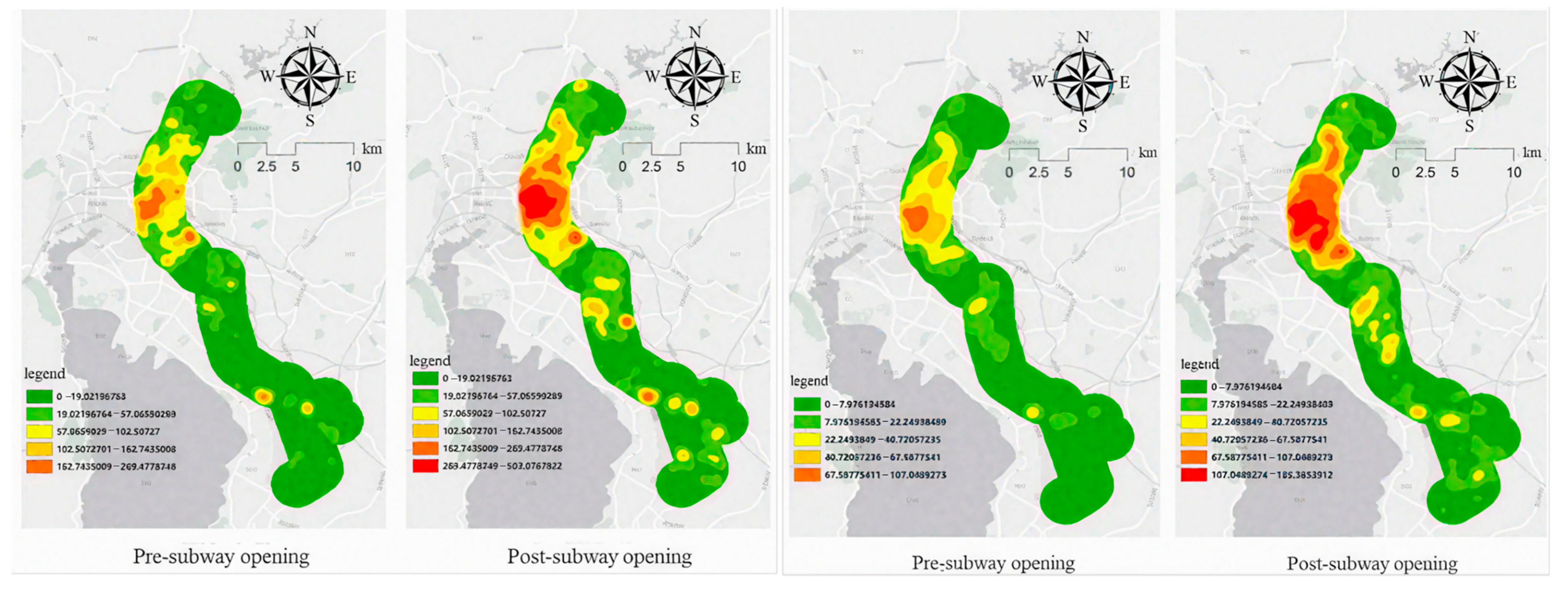
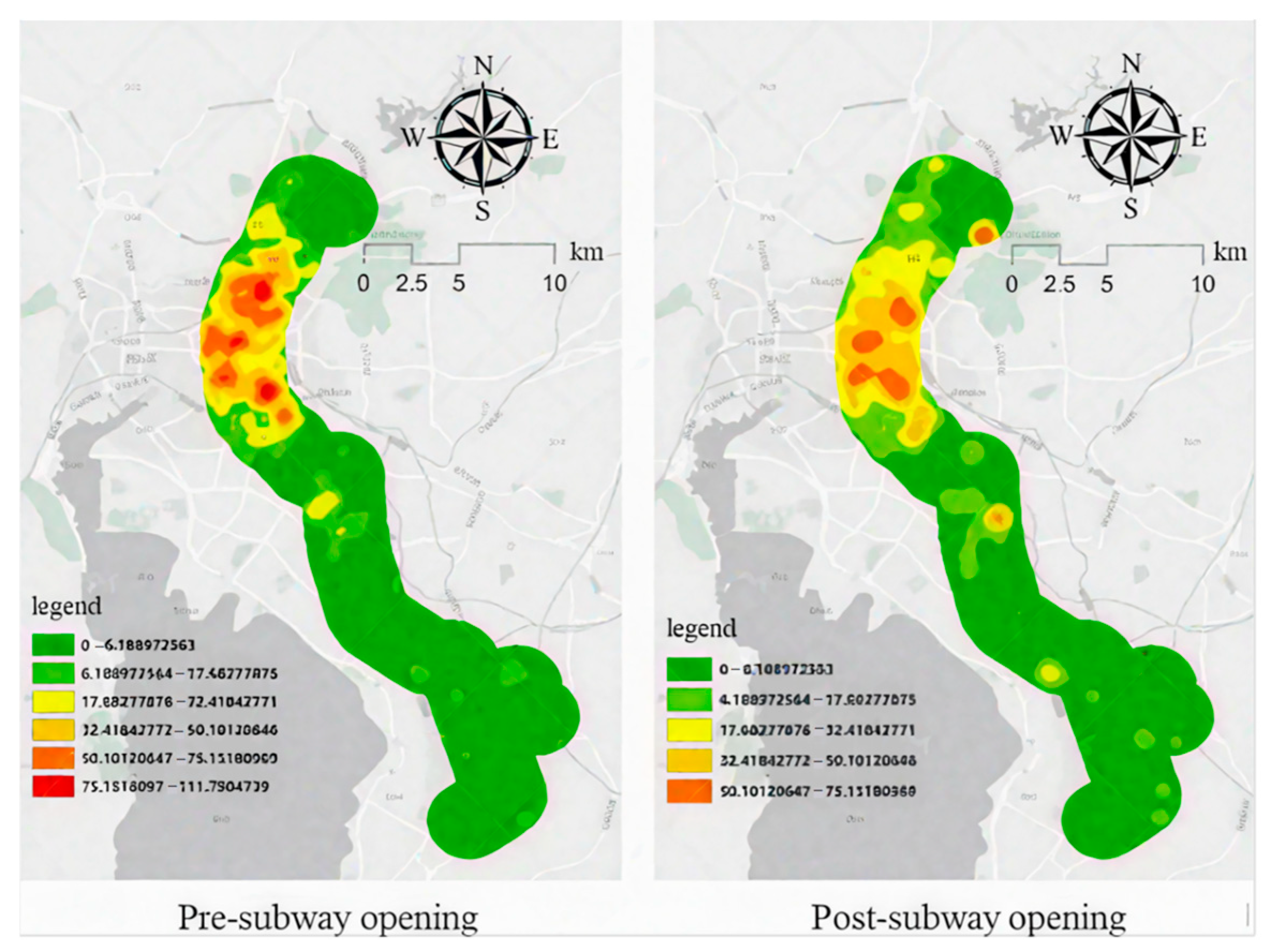
Firstly, the opening of the subway has a significant impact on the built environment of the surrounding corridors and stations, a fact that has been corroborated by previous research [
27]. After the subway opening, there is a noticeable increase in various amenities along its route, balancing out the distribution around the city center. There is a clear trend of increased land development and utilization. Land use at both ends of the line improves, with reduced facility density at stations, showing a clear stratification of the peripheral area.
Subsequently, the inauguration of the subway system has profoundly influenced the daily behaviors of residents living along its route. Notably, there has been an increase in the presence of highly educated, high-income individuals, and those with specialized occupational skills near the subway stations, alongside a significant rise in automobile ownership among local households—signals of the onset of gentrification. LIANG’s research also shows that the influx of higher-income, highly educated individuals and the outflow of lower-income residents are closely linked to the development of subway infrastructure [
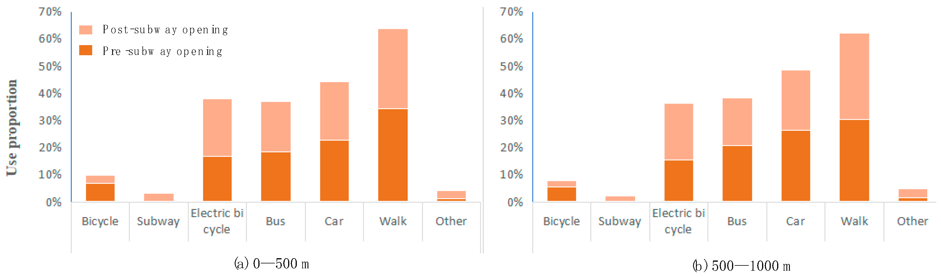
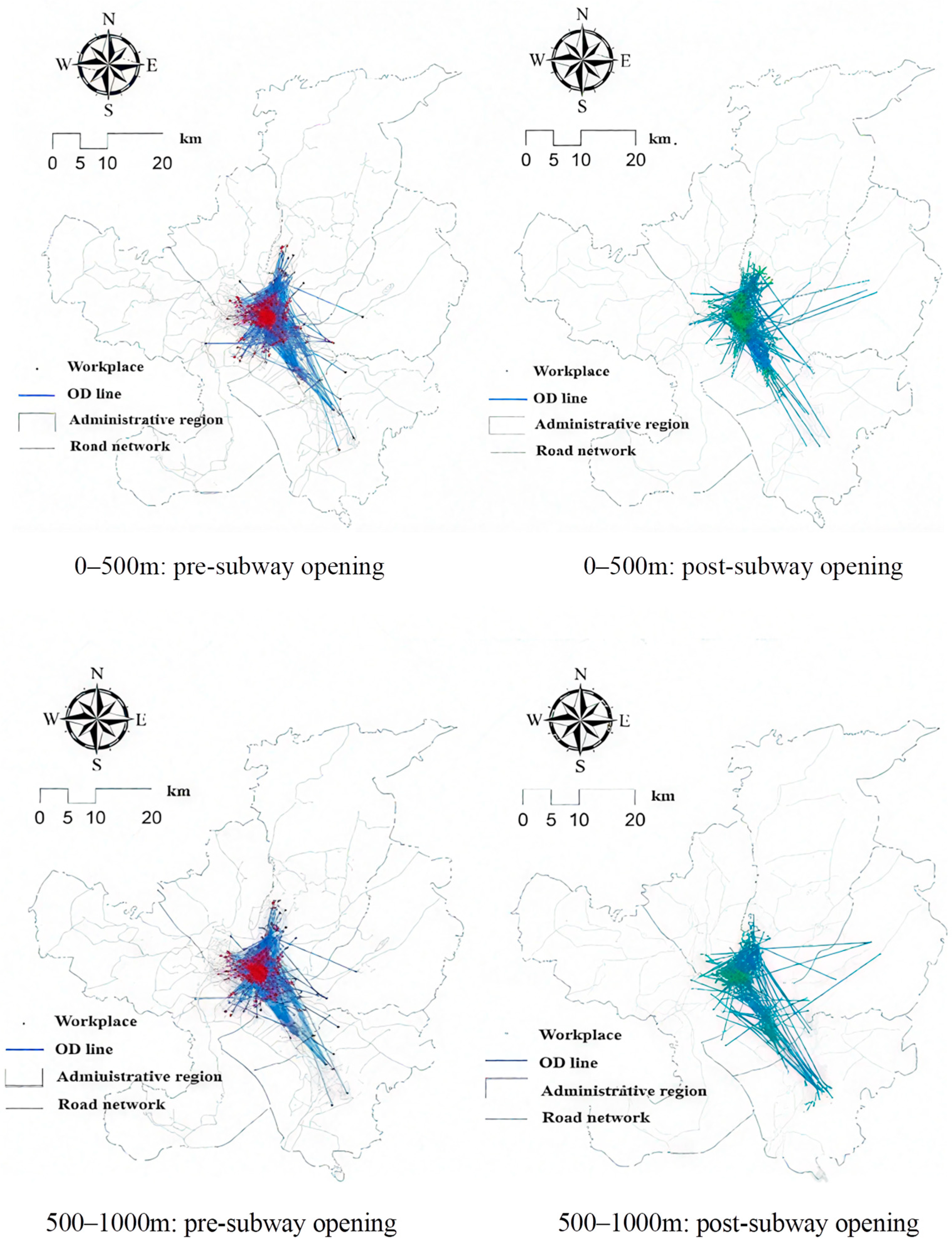
28]. Moreover, there has been a noticeable increase in the duration, span, and frequency of residents’ trips, particularly in areas near the subway stations. Upon adjusting for residents’ economic characteristics, significant differences in travel behavior across both time and space become apparent. In the inner circle, residents’ travel distances have decreased, their activity spaces have contracted, and their travel intensity has diminished—this stands in stark contrast to the outer circle areas. Furthermore, following the subway’s introduction, there has been a slight reduction in the proportion of car trips, indicating the subway’s role in curbing car usage. From a spatial perspective, the effect on car usage is more pronounced in areas farther from the subway stations. This contradicts the general pattern where the subway’s influence on car usage diminishes with distance from the stations. This phenomenon may be explained by the fact that residents in outer areas often face challenges such as limited coverage and infrequent traditional public transport options, such as buses. The subway’s opening has expanded their travel choices, especially during peak hours when the subway’s advantages over buses or private cars are most evident, contributing to a reduction in car usage.
Finally, the inauguration of the subway system fundamentally alters the mechanisms through which the built environment influences residents’ travel behaviors. In terms of temporal scenarios, there is an escalation in both the quantity and dimensions of pivotal variables, with bus proximity emerging as a notable dimension, thereby altering how the built environment shapes residents’ travel behaviors. Regarding spatial scales, factors such as design and diversity within the built environment begin exerting influence on travel behaviors in the inner sphere, whereas density gains prominence in the outer periphery. In terms of influence mechanisms, the inner built environment undergoes fundamental changes in its impact on residents’ behaviors, whereas in the outer periphery, the magnitude of influence varies. Regarding residents’ travel patterns and activity levels, pre-subway inauguration, high-density facilities shorten travel distances, increased land mixing extends travel distances and encourages automobile usage, while shopping amenities influence residents’ activity durations. Post-subway opening, high-density facilities and expanded station networks diminish residents’ travel distances, enhanced bus services extend travel distances while boosting public transit usage, and land mixing limits the escalation of activity durations.
6.2. Conclusions
This study on the impact of subway openings on residents’ travel activities has yielded several key findings. First, in comparison to the built environment, residents’ socioeconomic attributes have a relatively stable influence on travel behavior. This suggests that the built environment plays a crucial role in shaping residents’ travel behaviors, making it easier to guide and influence these behaviors. As a result, it is important to prioritize a comprehensive workflow for planning, developing, and post-evaluating the built environment in station areas. Second, the impact of the built environment on residents’ travel behavior varies not only by context but also across different spatial scales. Therefore, when planning and developing the built environment in station areas, attention should be given to location and scale factors, and land development strategies should be tailored to the specific characteristics of each station zone. Finally, after the subway opens, proximity to bus services significantly influences nearly all residents’ travel activities. This underscores the growing importance of public transportation as urban areas expand. Consequently, a dual approach is required, focusing on both enhancing physical infrastructure and improving service quality. These research conclusions and policy recommendations offer valuable insights for cities in the early stages of developing their rail transit systems.
Furthermore, this study is not without its constraints. The travel data of residents utilized in this study has been derived from a selected sample segment, and the survey method employed is a door-to-door RP survey, which may introduce bias into the residents’ self-assessment of their travel patterns. Hence, it remains uncertain whether these data can effectively capture the authentic travel behaviors of residents along the route. With the advent of the big data era, encompassing sources like mobile phone signals and GPS data, researchers are poised to provide more precise insights into individual daily travel activities, with future studies well-positioned to exploit this opportunity fully. Moreover, in contrast to panel data, the mixed cross-sectional data employed here offers limited insights into causality, thus warranting future investigations into the longitudinal dynamics of individuals within a narrow scope.


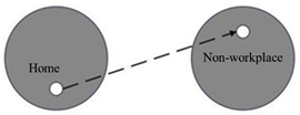

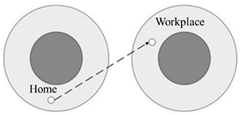

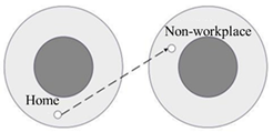
 0–500 m buffer zone
 500–1000 m buffer zone
 Travel orientation