Review

Submarine Terrain Generalization in Nautical Charts: A Survey of Traditional Methods and Graph Neural Network Solutions

1
School of Marine and Technology, Tianjin University, Tianjin 300072, China
2
Key Laboratory of Ocean Geomatics, Ministry of Natural Resources of China, Qingdao 266590, China
3
The School of Resource and Environmental Sciences, Wuhan University, Wuhan 430072, China
4
Institute for Marine Strategic Studies, Tianjin University, Tianjin 300072, China
*
Author to whom correspondence should be addressed.
ISPRS Int. J. Geo-Inf. 2025, 14(7), 257; https://doi.org/10.3390/ijgi14070257
Submission received: 30 April 2025 / Revised: 23 June 2025 / Accepted: 26 June 2025 / Published: 30 June 2025

Abstract

The generalization of nautical charts remains crucial in geographic information science and cartography. Traditional geometry-based methods have contributed to the advancement of automated generalization to a certain extent, but they still exhibit significant limitations in handling complex marine spatial relationships. This paper proposes the Graph Neural Network (GNN) as a transformative solution. GNN excels at processing non-Euclidean geospatial data, addressing the following three critical problems in the generalization of submarine terrain data: geographic feature representation, data processing, and the generalization process. The review first systematically outlines the main operators and fundamental methods of chart generalization. It analyzes their specific performance in various elements such as soundings, depth contours, islands, and coastlines. Subsequently, the potential of GNN is explored in addressing the limitations of traditional generalization methods. Although GNN is not a panacea, it shows advantages through horizontal and vertical comparisons. Finally, the challenges encountered in applying GNN to cartographic generalization are discussed.

1. Introduction

From early hand-drawn maps to modern automated digital mapping systems, cartographic generalization has formed its own set of theories and methods. It refers to the process of reducing a large-scale map to a small-scale map. According to the purpose of the map and the characteristics of the mapping area, the cartographer presents the regular characteristics and typical features of the mapping object in a general and abstract way, while discarding those features that are secondary or non-essential to the map. Chart generalization, a specialized application of this process, has specific requirements [1], as shown in Table 1.
Historically, the term ’Charts’ has generally referred to nautical charts, the oldest and most widely used type of charts. (Figure 1). Their main function is to help ships navigate safely by displaying relevant marine elements of the submarine terrain, such as soundings, depth contours, Digital Bathymetric Models (DBM), islands, reefs, and coastlines. Chart generalization applies operators and traditional methods to represent these elements more clearly, depending on the map’s purpose and scale. The research into nautical chart generalization combines traditional map generalization principles with algorithms specific to ocean-related elements [2].
The goal of generalization is to convey spatial concepts through graphic effects rather than simply reducing the amount of data [3]. Traditional chart generalization methods rely heavily on manual operations and local structural modifications [4,5]. With the advancement of data acquisition technology and the increased need for safe ship navigation, the area is facing growing limitations in geographic feature expression, data processing, and generalization efficiency.
To overcome these limitations, a shift toward automated, intelligent generalization methods is imperative [6]. Geospatial Artificial Intelligence (GeoAI), which is the intersection of spatial data and artificial intelligence [7], has been attempted in the generalization of submarine terrain data. Wang and Tian [8] first introduced artificial neural network technology for the automatic generalization of soundings. Furthermore, more recent machine learning-based approaches to depth contours [9,10] demonstrate this trend. However, beyond model complexity, effective generalization demands the incorporation of domain knowledge through advanced feature engineering [11]. GNN provides a potential solution for the intelligent production of nautical charts.
The purpose of this review is to provide an overview of the generalization of various types of submarine terrain data and their key issues, and to explore the potential of GNN as a solution. The existing traditional geometric methods still have limitations in terms of geographic feature representation, data processing, and generalization process. In addition, although there have been some reviews on the generalization of nautical charts, none of them have addressed the application of artificial intelligence. However, GNN has natural advantages as an advanced technique capable of capturing complex spatial relationships and multi-scale features. More importantly, although the advantages of GNN in graph structure data processing have been widely studied, the application prospects and the advantages and challenges of GNN in the field of generalization have not been fully summarized. Therefore, we start from the basic theory of a nautical chart, review the classical methods of chart generalization and their application based on the limitations of the traditional methods, and discuss the promising research contents inspired by GNN for solving these problems.
This study is divided into the following five parts:
  • The basic theory and methodology of chart generalization and GNN;
  • A review of the generalization of various types of submarine terrain data;
  • Discussion of the limitations of the classical methods in cartographic generalization, with case studies to illustrate how GNN can effectively deal with these challenges, especially in terms of geographic feature representation, data processing, and the generalization process;
  • Introduction to the advantages and challenges of GNN. By comparing different GNN architectures vertically and comparing them horizontally with other popular architectures. The advantages of GNN in cartographic generalization are shown. The challenges of developing GNN in the context of submarine geomorphology generalization are presented;
  • The concluding remarks are presented.

2. Fundamental Knowledge on Chart Generalization and GNN

2.1. Main Operators for Chart Generalization

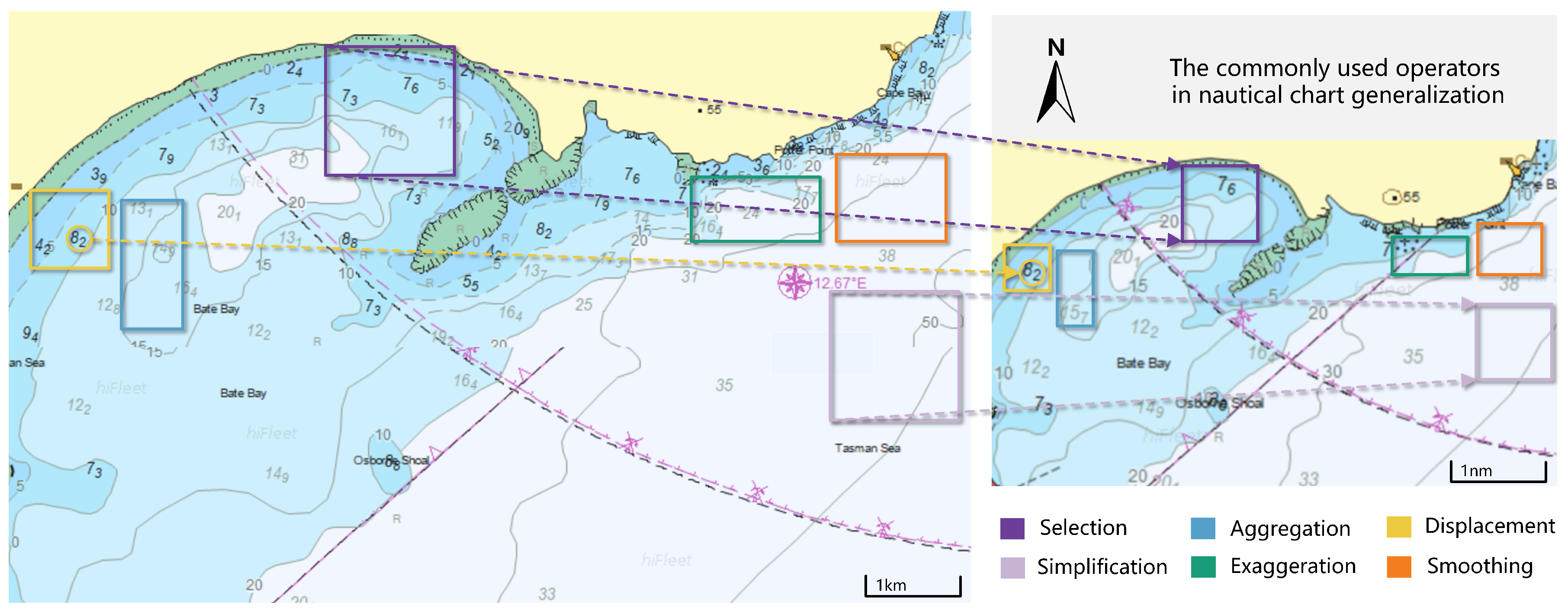
The operators of cartographic generalization constitute a complete and orderly process of cartographic generalization as shown in Figure 2. These methods are distinct yet interrelated, and under certain circumstances, they can be transformed into one another.
Selection is the most fundamental and important method in cartographic generalization. The first meaning refers to the selection of content elements, which means choosing specific types of information that are essential and relevant according to the chart’s subject matter and intended use. The second meaning is the selection of ’cartographic’ objects, such as the selection of meaningful soundings from a large number of them.
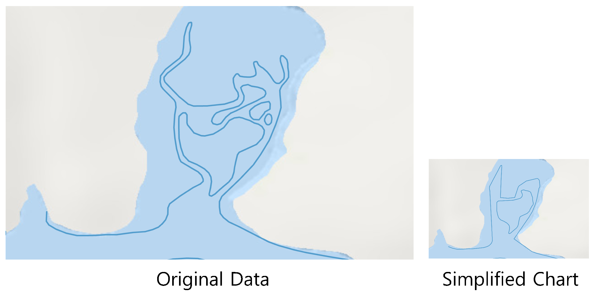
Simplification refers to the reduction of the geometric complexity of cartographic elements, replacing complex shapes with simpler ones (Figure 3). In the production of nautical charts, due to scale reduction, the shapes become smaller and curves increase, and this hampers the display of their key features. Alternatively, due to the differences in chart themes and purposes, certain details may not need to be represented. The goal of simplification is to retain the characteristic contours of the object and display the features that are essential from the perspective of the chart’s purpose while maintaining clarity and readability. For areal features, simplification applies both to the external boundary and to the internal structure.
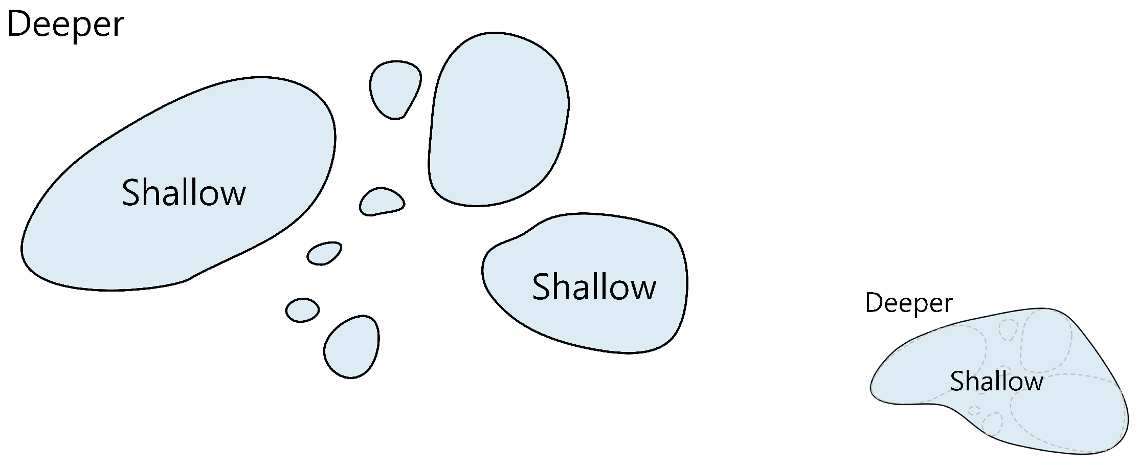
Aggregation is the process of combining parts of similar objects that are very close to each other. For example, when multiple adjacent depth contours represent the same submarine terrain feature and the distance between them is very close, these lines can be merged into one depth contour to improve the readability of the map (Figure 4).
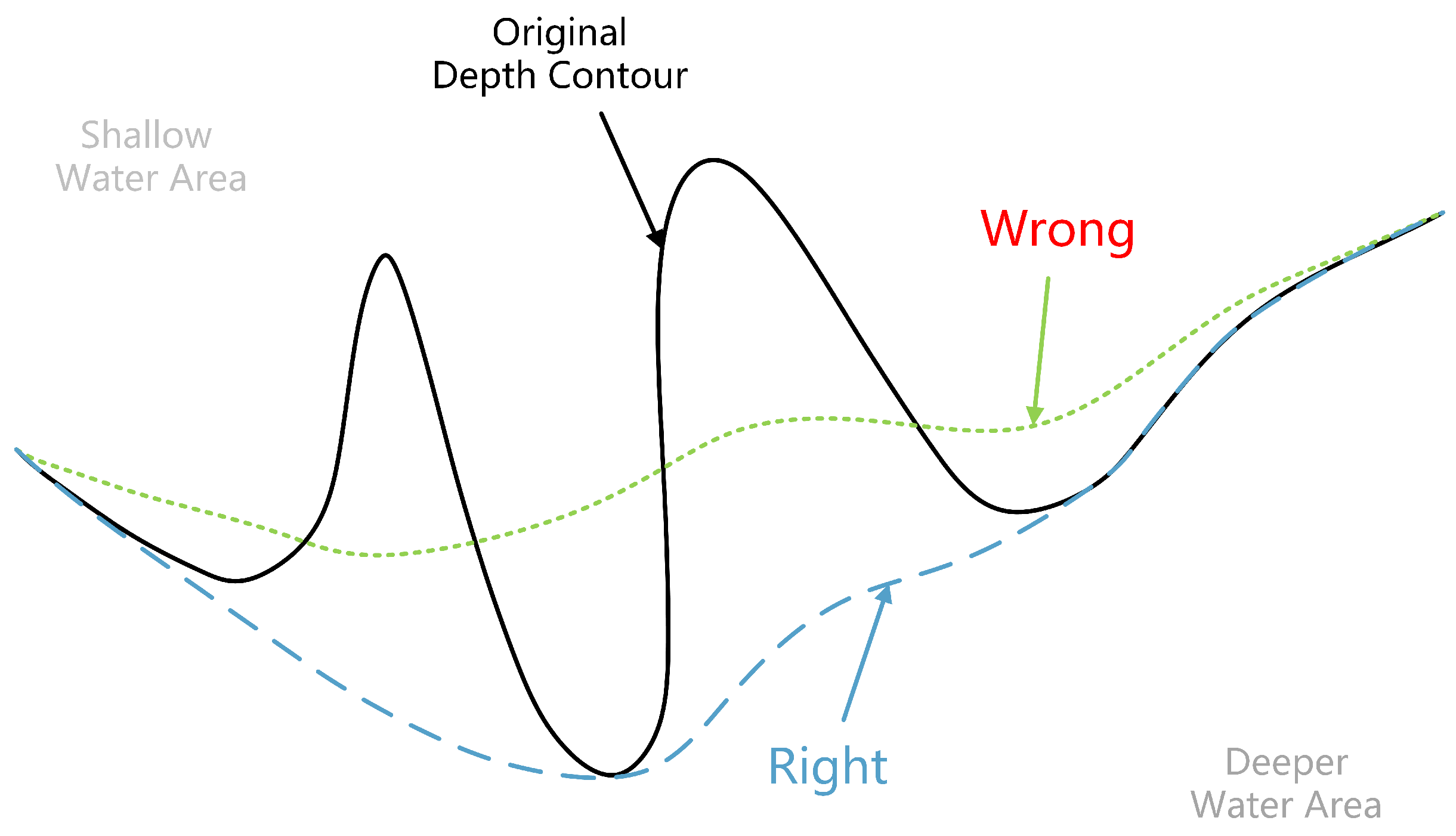
The essence of generalization is the deletion of details, but individual details are to be retained in a particular context. To meet navigation safety needs, the process must comply with the principle of ’expansion of shallow water and reduction of deep water’. That is, depth contours can only be displaced and deformed towards deeper water.
Displacement involves shifting the position of secondary objects to maintain the basic spacing between symbols. When the source data are scaled down to the new chart scale, they will inevitably lead to crowding or even overlapping of symbols. Therefore, in addition to reducing the symbol size, the most commonly used method is displacement.
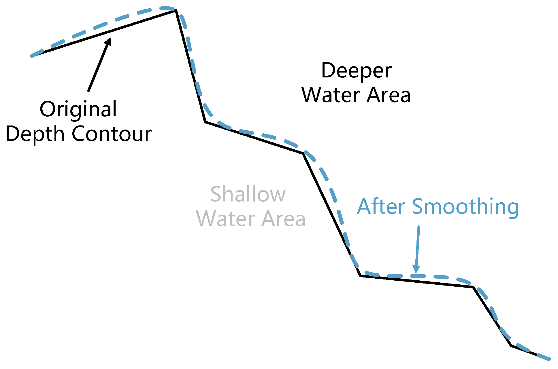
Since depth contours are typically stored as polyline segments formed by a sequence of coordinates, and during data compression and partial simplification, some nodes may be removed, this inevitably leads to noticeable angles along the lines. Smoothing is a technique that fits the original polyline by smoothing the curve, as shown in Figure 5. Its core purpose is to eliminate sharp corners in the polyline, thus giving the curve a smoother and more elegant appearance.

2.2. Traditional Methods of Chart Generalization

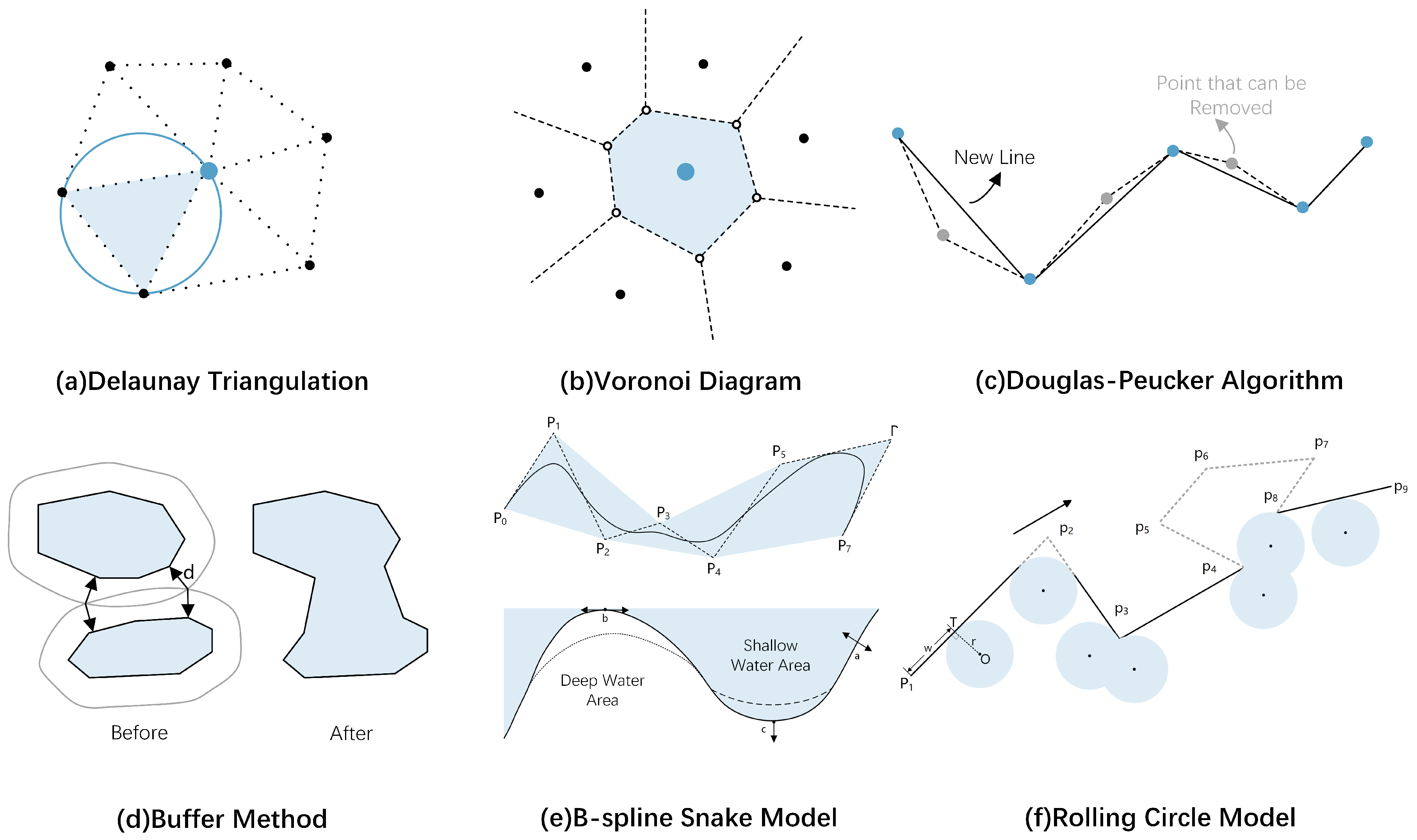
Traditional methods have been widely used in the generalization of various types of submarine terrain data due to the growing demand for nautical charting. These methods mainly focus on geometric elements such as points, lines, and areas, and they realize the extraction and expression of geographic features through operators. However, they still have some limitations. A review of the relevant literature was conducted (Figure 6), and several commonly used classical methods were selected for study, with their schematic diagrams shown in Figure 7, showing the value of chart generalization with practical application examples. Relevant studies of these methods in chart generalization are shown in Table 2.
The characteristic of Delaunay triangulation is that the circumscribed circle of any triangle does not contain other points. This method can effectively maintain the proximity relationship between elements, as shown in Figure 7a. Let P = { p 1 , p 2 , , p n } be a set of discrete points on a plane. The goal of Delaunay triangulation is to generate a set of triangles T such that the intersection of any two triangles in T is either empty, a common vertex, or a common edge. The triangulation must satisfy the empty circumcircle property and the maximization of the minimum angle criterion. Specifically, for any triangle p i p j p k T , its circumcircle must not contain any other point in P. This property can be mathematically expressed as follows:
Circumcircle ( p i p j p k ) P = { p i , p j , p k }
This ensures the fatness of the triangles, avoiding the formation of skinny or elongated triangles. The second criterion can be described by maximizing the minimum angle among all triangles in the triangulation. Let θ i j k denote the interior angles of triangle p i p j p k , then the minimum angle θ min satisfies the following:
θ min = max T min p i p j p k T θ i j k
In the generalization of depth contours, the scatter set composed of nodes on the contours can be used as the basis for constructing constrained Delaunay triangular nets using line segments on the contours as constraint edges, thus realizing the aggregation of neighboring depth contours.
A Voronoi diagram is based on a point set [28] and divides the plane into polygonal regions centered on the generating point (Figure 7b). Voronoi diagrams and Delaunay triangulation have a dual relationship. Given a set of generator points P = { p 1 , p 2 , , p n } , the Voronoi diagram partitions the plane into regions, where each region V ( p i ) corresponds to a point p i P . The Voronoi region V ( p i ) is defined as follows:
V ( p i ) = { x R 2 d ( x , p i ) < d ( x , p j ) , j i }
where d ( x , p i ) denotes the Euclidean distance between point x and the generator point p i . In this way, the entire plane is divided into polygonal regions centered around each generator point. Voronoi diagrams can be used to analyze features such as adjacency and distribution density. In island and reef generalization, Voronoi diagrams can be applied to identify the density of islands and remove islands with higher density until the selection number target is reached [23].
The Douglas–Peucker algorithm takes the start and end points of the original curve as the base straight line, calculates the perpendicular distance from each point on the curve to the straight line in turn, and if the distance of a point exceeds a preset threshold, the point is retained as a characteristic point of the curve. It divides the curve into two segments, and it recursively repeats the above process for each segment of the curve, as shown in Figure 7c. Given a curve C = { P 1 , P 2 , , P n } with start point P 1 and end point P n , the perpendicular distance d i from each point P i on the curve to the baseline segment P 1 P n ¯ is computed as follows:
d i = ( P n P 1 ) × ( P i P 1 ) P n P 1
If the maximum distance d max among all d i exceeds a given threshold ε , the corresponding point is retained, and the curve is divided into two segments as follows: from P 1 to P i and from P i to P n . The same procedure is then recursively applied to each segment. If d max ε , all intermediate points between P 1 and P n are discarded, and only the end points P 1 and P n are preserved.
The Buffer Method is used to generate a buffer region of a specified distance around a target element, which can realize the effective control of the space around the element by adjusting the size of the radius d [36,46]. For example, the aggregation of depth contours was shown in Figure 7d. Given a set of geographic features O = { o 1 , o 2 , , o n } and a predefined buffer radius d, the buffer zone B ( o i ) of each feature o i is defined as follows:
B ( o i ) = { x R 2 d ( x , o i ) d }
where d ( x , o i ) denotes the Euclidean distance between point x and the target feature o i .
The B-spline curve can provide local control and smoothness. A B-spline curve is defined by a set of control points and basis functions. Given a set of control points P = { P 1 , P 2 , , P n } , the B-spline curve C ( t ) can be expressed as follows:
C ( t ) = i = 1 n N i , k ( t ) P i
where N i , k ( t ) denotes the B-spline basis function, k is the order of the curve, and t is the parameter. The snake model realizes shape deformation by minimizing the energy function and finally generates an optimized curve that meets the external constraints [43]. The B-spline snake model combines the advantages of both (Figure 7e).
With the Rolling Circle Model it is possible to retain the main shape characteristics of the curve while achieving the generalization of the curve on one side [41]. The basic equations and procedures of the rolling circle model are as follows. The coordinates of the center O of the rolling circle are computed based on the following conditions:
T O · P 1 P 2 = 0
T O = r
Solving these equations yields the following:
O = P 1 + w · P 1 P 2 P 1 P 2 + T O
where r is the radius of the rolling circle, and w is a rolling factor. When the rolling circle intersects with other parts of the curve, it is necessary to compute the tangent point T. Special cases also exist. For example, when the rolling circle encounters a convex corner, a rotation factor is introduced to calculate the rotated position of the circle center. In the case of a sharp corner, it must be determined whether the tangent point lies on the segment. If not, the final tangent point is determined using the perpendicular intersection method. The generalization of coastlines needs to take into account the principle of “expanding the land and reducing the sea”. The rolling circle removes small bays and tiny depressions by rolling one side of the coastlines, while retaining the main headlands, ensuring that the integrated coastline meets the requirements of navigation safety, as shown in Figure 7f.

2.3. Graph Neural Network

In the generalization of depth contours (edges) and soundings (nodes), the topological relationships established using methods such as Delaunay triangulation in undirected graphs can effectively represent submarine terrain, aligning well with the structure of graphs in graph theory. The graph structure can connect discrete soundings and represent their abstract relationships in the form of edges. Based on this, the distribution range and density of soundings clusters can be identified, enabling their rational partitioning.
A graph consists of vertices (nodes) and edges that connect the nodes and can be represented by the following equation:
G = ( V , E )
where V denotes nodes and E denotes edges. It should be emphasized that edges can be weighted or unweighted, directed or undirected [12].
The adjacency matrix and adjacency table can be used to represent the graph. The element of the adjacency matrix represents the connection between the nodes. Sparse matrices are typically used to improve computational efficiency, retaining only the indices and values of non-zero elements. The other representation method is the adjacency list, which stores the neighboring nodes of each node or stores the edges between all pairs of nodes.
The latest achievement of graph theory in deep learning (DL) is the Graph Neural Network (GNN), which can thus be explored for nautical chart generalization. In GNN, graphs are typically used to represent the relationships (edges) between entities (nodes). The core idea is to update node features through a differentiable message passing mechanism. Each node v i has a feature vector h i R d , and its feature representation is updated by passing messages to and from its neighbor nodes. Specifically, the message passing consists of two operations. First, each node collects messages from its neighbor nodes using the following equation:
m i ( l ) = v j N ( v i ) f M h i ( l 1 ) , h j ( l 1 ) , e i j
N ( v i ) represents the set of neighbors of node v i , e i j denotes the edge weight between node v i and node v j , and f M is the message aggregation function, typically a differentiable neural network. Subsequently, the features of the node are updated in the following step:
h i ( l ) = f U ( h i ( l 1 ) , m i ( l ) )
where f U is the update function, which can also be a neural network. The features of the nodes are progressively updated through this message passing mechanism, capturing both local and global information in the graph structure.
The Graph Convolutional Network (GCN) is a convolutional neural network that can act directly on graphs and utilize their structural information. It uses convolutional operations to aggregate feature from neighbor nodes. It performs convolution in the spectral domain of the graph to effectively update node features, with the update rule given by the following formula:
h i ( k + 1 ) = σ j N ( i ) { i } 1 d i d j W h j ( k )
where d i and d j represent the degrees of nodes v i and v j . W is the parameter of the convolutional transform, which is called the weight matrix. Furthermore, σ is the activation function. The advantage of GCN lies in its high computational efficiency and its ability to effectively capture local structures in the graph. Its design inspiration comes from spectral graph convolution, where the convolution operation is simplified using a local first-order approximation, thus avoiding the high computational cost of frequently calculating eigenvalues and eigenvectors in spectral graph convolution.

3. Generalization of Various Types of Submarine Terrain Data

The generalization of various types of submarine terrain data are often regarded as a relatively independent and special research content in map generalization [47]. It mainly includes several types, such as soundings, depth contours, coastlines, islands, and reefs.

3.1. Generalization of Soundings

In the production of digital nautical charts, distribution patterns and the density of soundings are critical factors influencing the information capacity and submarine topographic features. Therefore, the generalization of sounding can follow the principles outlined as follows [13,48]:
  • Taking the shallow soundings and leaving the deeper soundings so as to ensure navigational safety.
  • Focusing on the selection of important soundings that can reflect the channel and other negative seabed topography.
  • Rational distribution of soundings should be in the form of a diamond as far as possible. The ratio of the rhombus should be adjusted according to the requirements.
  • The selection of soundings should be harmonized with other elements such as coastlines and depth contours.
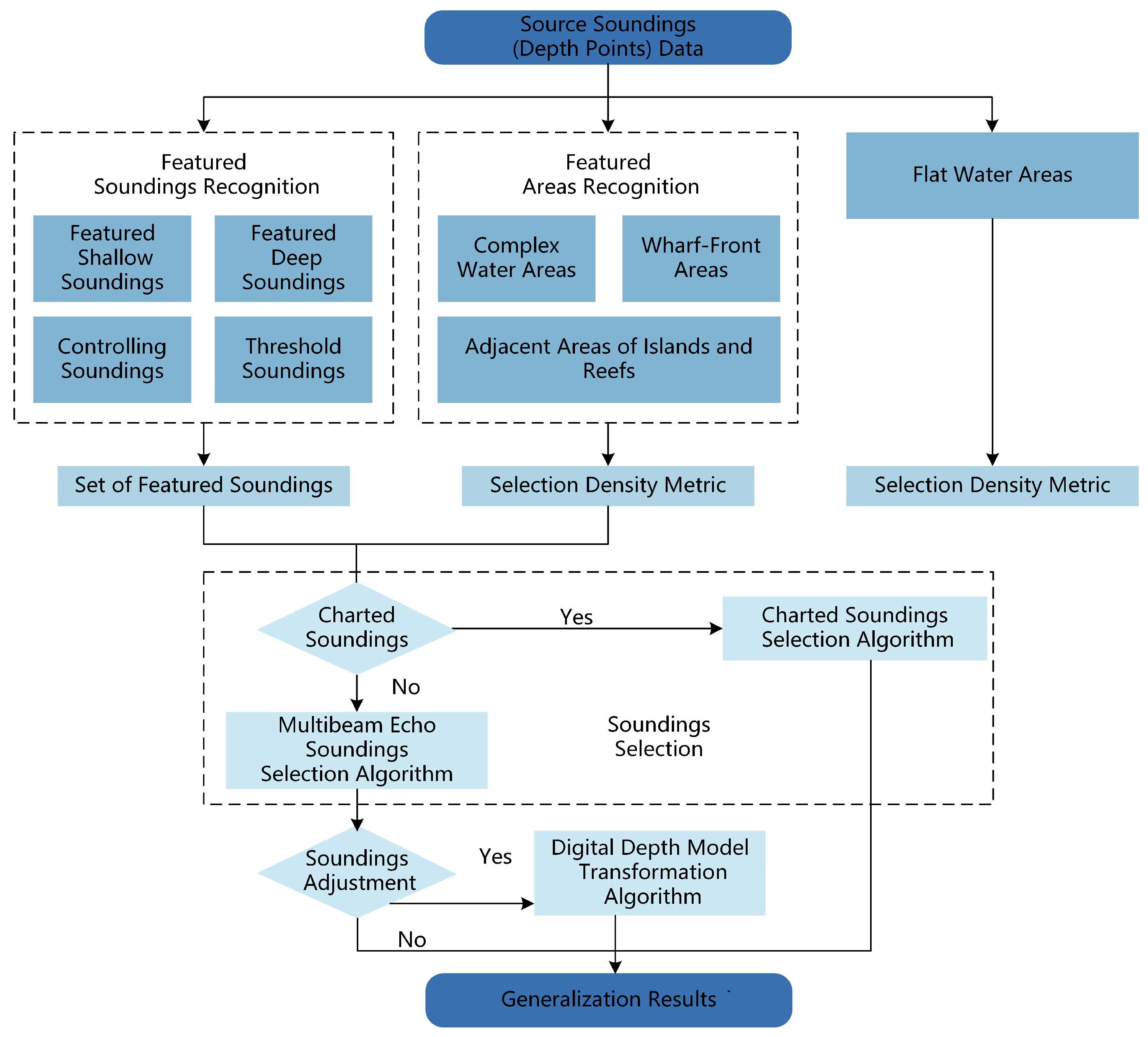
The general process for the selection of soundings is shown in Figure 8. According to the different data sources of the soundings, it can be divided into the generalization of the soundings based on the cartographic products, the bathymetry survey results, and the Digital Bathymetric Models.

3.1.1. Sounding Generalization of Cartographic Products

The soundings used in cartographic products refer to the bathymetric data that comply with charting standards, typically derived from previously published nautical charts (Figure 9), and these are in ‘.000’ file format. Soundings are a collection of discrete points used to describe changes in submarine terrain [49]. The generalization of soundings is not a simple point selection based on geometric features but emphasizes the importance of context, which means the complexity of the bathymetric changes shown in the study area should not be changed [12]. Conventional algorithms often control point density based on radii or grids [50]. This reduces effectiveness and does not meet the requirements of navigational safety and clarity. Label-based methods offer a solution to this issue [51].
From the point of view of topographic characteristics complexity [52], the models introduce Delaunay triangulation, the Voronoi diagram, the 3D surface bi-directional buffer model, and the Triangulated Irregular Network (TIN) to divide the seafloor topography into subregions and use “bathymetric trees” to represent the topological relationships in different depth ranges [14,18,38]. Important areas of topographic features can be automatically identified for the generalization of soundings.

3.1.2. Sounding Generalization of Bathymetry Survey Results

Sounding generalization based on bathymetry survey results mainly focuses on the thinning algorithms of Multibeam Echosounder (MBES) data. Highly accurate bathymetric data provide a reliable basis for chart mapping [53,54]. Figure 10 shows the results after 3D visualization of the multibeam measurement data. The density of soundings in MBES has a large impact on the fine reading of the generated seafloor terrain model [55]. However, the dense and large number of point clouds produced by the survey is much greater than the number of soundings that can be carried by a nautical chart [54]. The selection of bathymetric data not only needs to reduce the data density, but it should also conform to the application scenarios of charts and preserve the changes in seafloor topography [47].
The research covers the optimization of data compression and structure, extraction of topographic features, coordination of soundings and depth contours, and navigational safety constraints. For example, Wen et al. [56] and Wang et al. [57] mathematically solved the data density control problem. Furthermore, to meet the needs of cross-scale mapping, the hierarchical selection strategy can be used [58,59,60]. In terms of grid structure optimization, a method for selection based on Delaunay triangulation and dynamic rhombic grids was proposed earlier [61].
In the second place, the extraction of submarine terrain features can also be used to select soundings. Huang et al. [26] first formalized the constraints involved in the generalization of topographic features. Li et al. [15,18,59] designed a profile line-based feature sounding extraction method based on the alignment characteristics of MBES, combining the optimized results of rhombic search with slope, slope direction [16], and sounding values. Efficient operations can also be achieved by studying the topographic features of complex areas such as convex land, concave land, and deep troughs for segmentation and identification [17,23].
In addition, to ensure the rationality and consistency of the distribution of soundings and depth contours, Jia et al. [33] optimized the selection of feature points by defining the degree of coordination between the two in combination with the Douglas–Peucker algorithm. A generalized model based on an extended detection tree [62] generates depth contours through triangular mesh decomposition to represent the seafloor topography more accurately. Ultimately, these studies lay the foundation for safeguarding the safety of ship navigation.
Last but not least, in terms of navigational safety and constraints, a variety of innovative safety verification and assessment methods have been developed [63], which can more accurately evaluate the rationality of the distribution of points in the generalization results.

3.1.3. Sounding Generalization of the Digital Bathymetric Model

The Digital Bathymetric Model is a three-dimensional digital seafloor model constructed by interpolating the soundings from the survey results [47], which are digital representations of the seafloor surface morphology and are widely used in chart mapping. The generalization of DBM can be divided into two categories as follows: model compression and model transformation.
Compression is mainly realized by the reasonable deletion of water depth data constituting the model or selection of data meeting the requirements of the target scale, which will not change the original bathymetric values and ensure the consistency and reliability of the data [32]. The transformation of DBM is realized by adjusting the water depth to change the morphology. The problem of traditional bathymetry interpolation is that it does not take into account the difference in complex seafloor topographic regions [64,65,66].

3.2. Generalization of Depth Contours

Creating high-quality depth contours requires generalization, i.e., a meaningful streamlining of what polylines express [67]. The generalization of depth contours can be broadly divided into the following two categories: those based on geometric elements and those based on submarine terrain patterns. Its generalization algorithm should be guided primarily by the following principles:
  • The trend of depth contours before and after generalization must remain consistent with the primary characteristics of the seabed topography.
  • In the process of generalization, it is necessary to make the area of shallow water larger than that before generalization and the area of deep water smaller than that before generalization, i.e., “expansion of shallow water and reduction of deep water” (Figure 11), in order to ensure the safety of navigation.
  • Topological errors such as intersections, self-intersections, and mutual overlapping of depth contours should not occur.
  • Only essential information should be retained and presented in a clear and understandable manner.

3.2.1. Generalization Based on Geometric Elements

Depth contours belong to one of the line elements. The goal is to reduce the number and simplify the line contours. The generalization based on geometric elements is mainly done through the following three types of methods: node simplification, bending identification and optimization, and line element smoothing to ensure that it meets the requirements of navigational safety and cartography while maintaining the topographic features [68].
The first type of methods mainly focuses on achieving simplicity by reducing the number of redundant nodes that make up the polylines [34]. To solve the problem of multiplicity, Xing et al. [69] used node ordering to quickly generate depth contours based on the study of Wu et al. [70].
The second type of methods typically simplifies depth contours by focusing on the curves within the contours as the basic unit. By removing unnecessary bends, these methods better preserve key shape feature and enhance the readability of nautical charts. Wang and Müller [71] proposed a line feature generalization method based on curvature shape analysis. Li et al. [19] designed different recognition and processing methods for three types of depth contour curves that need simplification (small complete bends, small incomplete bends, and narrow “bottlenecks”). Tang et al. [42] developed a depth contours simplification model for field reclassification based on line element complexity [72].
The third method focuses on smoothing the depth contours to ensure the smoothness of the lines and meet the requirements of navigation safety. Li [18] proposed a smoothing method based on Bezier curve fitting [73], which ensures the smoothness of the depth contours and retains the terrain characteristics. The B-spline curve combined with the snake model, ensures even more the smoothness and morphological consistency of the lines and the topological correctness of the generalization of the graph [43,44,74]. Building on this, Miao and Calder [45] used a cubic B-spline snake model for the progressive generalization of depth contours to further enhance the smoothness of the lines.

3.2.2. Generalization Based on Submarine Terrain

The geomorphology-based methods focus more on how to make the extracted depth contours more accurately represent geographic features. The first approach is to generalize the seafloor surface and extract depth contours from the simplified surface [27]. This method belongs to model generalization, allowing the generation of depth contours at various scales, and it is characterized by stability and high speed. The current trend, i.e., the second method, is the direct generalization of raw depth contours derived from large-scale nautical charts or extracted from high-resolution DBM [18,19,20,75,76].

3.3. Generalization of Coastlines

Coastlines and islands and reefs are key to the landward extension of submarine terrain and the transition to them [77]. The following principles need to be followed when generalizing coastlines [78]:
  • It should be ensured that the position of the connection point of the polyline is accurate because they are the skeleton of the coastlines.
  • Shape maintenance: Coastlines should maintain the curved shape and outer contours of the graphic.
  • “Expanding the land and reducing the sea”: Priority should be given to retaining important headlands and discarding smaller bays. In some special cases, they can be appropriately exaggerated. It is particularly important in the production of large-scale nautical charts and must be strictly observed.
Common approaches in the generalization of coastlines include methods of shape preservation, simplification based on scale structure, simplification based on buffer feature points, and the treatment of artificial coastlines as distinct from natural coastlines.
The goal of shape-preserving methods is to preserve the shape characteristics of the original line [36]. For example, Christensen [79] proposed a method based on waterline and medial-axis, which effectively preserved the shape characteristics of the natural coastline. Furthermore, Lewin’s [80] perception-driven shape evolution method avoids morphological distortion caused by oversimplification by removing local details while retaining the overall structure. In addition, compared with the widely used Douglas–Peucker algorithm, the method of gradually eliminating points with less influence based on “effective area” is more suitable for simplifying complex curves [81].
The simplification methods based on scale and structure, on the other hand, focus on the analysis of multiple scales and the treatment of complex bending structures. An estuarine bay skeleton line model can effectively cope with the complex bending in the coastlines and realize the asymptotic simplification of the coastlines at different scales [82]. Similarly, Huang et al. [24] and Ai et al. [21] proposed simplification algorithms for complex geomorphology (e.g., estuarine bays) based on previous work [83]. A multi-branching tree structure rather than a binary tree [84] is used to deal with curved structures to improve the accuracy and reliability of the simplification effect.
The third method mainly uses buffers and feature point extraction to simplify the coastline and maintain the shape [22,36,85]. In practice, there are differences in the treatment of artificial and natural coastlines. The key to the generalization of natural coastlines is to manage the resolution, maintain the shape, and pay attention to the details of the islands [76].

3.4. Generalization of Islands and Reefs

Islands and reefs are important geographical elements in nautical charts, usually represented by points or polygons. Island selection is subject to the following conditions:
  • No isolated islands are allowed to be discarded at any scale, regardless of size.
  • If it is not possible to accurately plot small islands clustered together or close to the coast at the scale, they may be represented by black dots of a certain diameter.
Island generalization mainly involves quantity selection, group structure selection, and shape simplification. In terms of quantity selection, the open square root model is mainly used at present [29,86]. On the other hand, the selection of island group structures requires the correct identification of their spatial distribution characteristics and the retention of important island group patterns. This requires simultaneous attention to the prominence of individual islands as well as to the characteristics of large-scale typical islands and small-scale special island structures. Gestalt theory delves into the laws of how humans perceive overall group characteristics rather than focusing only on individual objects. It can categorize island structures according to size and shape based on experimental results [25,87]. Compared with the traditional Voronoi diagram method [23,28], the influence domain (IID) model and buffer growth model can more accurately identify the island distribution in high-density areas, retain isolated islands, and effectively reduce visual conflicts [30,39,40].
In terms of shape reduction, Zhu and Lu [31] used geometric means such as extreme value windows and minimum convex hulls to achieve automatic generalization of islands, and Anderson-Tarver et al. [88] introduced fuzzy set theory for terrain modeling to identify areas to be preserved in map synthesis, especially the shape features of archipelagos. The method is mainly used to deal with ’area patches’ [89], which are similar to wetlands and marshes. Adaptation thresholds are determined by dimensional estimation so that the degree of simplification of each patch adapts to its complexity [37,90].
From the review of classic methods and multi-factor submarine topography generalization, it can be observed that there are still some obvious limitations. Table 2 summarizes the performance of specific applications of Delaunay triangulation, the Voronoi diagram, the Douglas–Peucker algorithm, the buffer method, the rolling circle model, and the B-spline snake model in sounding, depth contour, island, and coastline generalization.
Marine elements in nautical charts often show complex spatial dependencies. Figure 12 illustrates vectorized submarine terrain data. These elements do not follow Euclidean geometric rules but rely on a more flexible spatial structure. These relationships can be naturally represented by the graph structure. GNN, as the latest achievement of graph theory in the field of DL, has become an important tool for processing complex graph structure data. GNN is able to effectively capture the relationship between nodes in the graph and update the features of nodes and edges through a message passing mechanism. This gives GNN a natural advantage in dealing with geographic feature representation, data processing, and the generalization process. Thus, the adoption of GNN for nautical chart generalization can automate the learning of relationships between nautical chart elements and optimize the representation of depth contours and the connection of soundings. At the same time, GNN can improve the accuracy and efficiency of the generalization result, providing a new solution for the intelligent production of nautical charts.

4. Critical Problems and Graph Neural Networks as Solutions

Overall, the solution for chart generalization using GNN stems from the following two aspects:
  • GNN is capable of learning multiple features of non-Euclidean data.
  • Geometric elements in a chart can be conceptualized as graph structures to address the unique challenges associated with cartographic generalization.
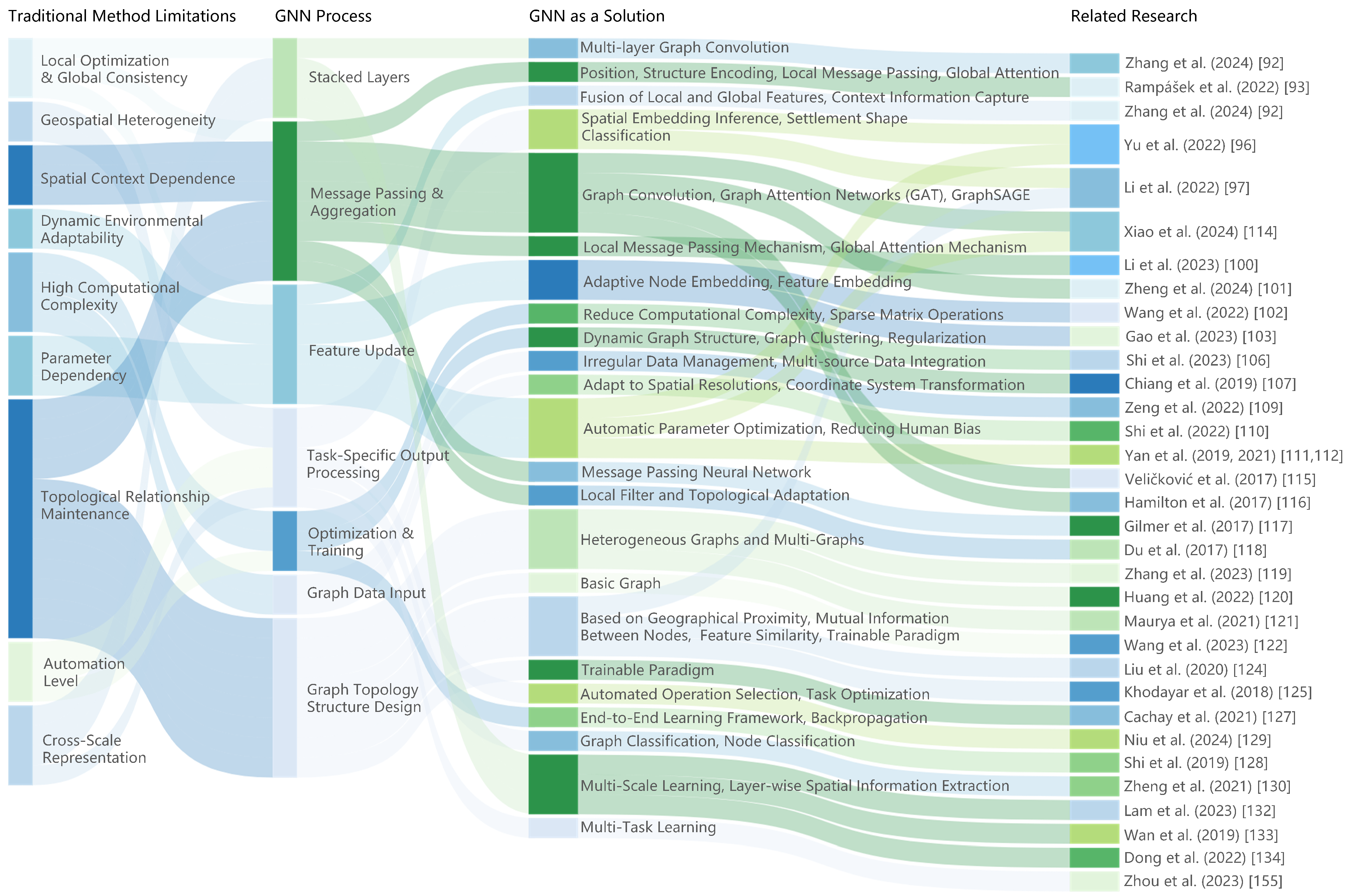
Figure 13 illustrates the relationship between the limitations of traditional chart generalization methods and solutions for the application of GNN in chart generalization. The theoretical rationale for addressing the various challenges in each of the GNN processes is outlined, and application cases supporting these choices are provided for reference.

4.1. Geographic Feature Representation

The core idea of nautical chart generalization is to accurately represent seafloor topographic features and ensure the safety of ship navigation [52]. Unlike the translational invariance of visual data features, changes in submarine topography are directly related to geographic location. GNN is good at mapping different locations and can introduce the location information as node or edge attributes. Overall, GNN addresses the challenges of representing seabed geographic features by combining local message passing and global attention mechanisms. It enables spatial embedding inference for unseen locations during the testing phase and supports context-aware feature extraction and aggregation.
To start with, existing generalization methods tend to again optimize to some extent the local features of a single geometric element (e.g., point or line or surface). However, these methods are relatively incapable of coordinating and processing global features of submarine topography. This may result in accidental deletions or overlaps, ultimately leading to distorted generalization results. GNNs generate flexible vector representations for nodes, edges, and the entire graph. Information is shared between nodes and edges within the GNN layer using a message passing mechanism that is capable of handling both local and global features. Local and global features can also complement and interact with each other [91]. GNNs integrating global and local features are able to classify more accurately [92]. For example, features describing the overall shape and features describing the local morphology of individual parts are effectively fused through a weighted graph structure and multilevel graph convolution. Moreover, Graph Transformers can encode both position and structure. They utilize local message passing and global attention mechanisms to optimize local features and ensure global consistency [93]. Besides, GCNs incorporating gated recurrent units (GRUs) are able to consider both local and global features for information propagation [94].
Furthermore, geographic heterogeneity reflects significant differences in the topographic characteristics of different regions [95], which are particularly pronounced in different marine areas. For example, offshore regions typically exhibit flatter continental shelf topography with relatively gentle changes in water depth, whereas pelagic regions may contain steep submarine mountains with great changes. Traditional generalization methods often assume that the geographic environment is relatively homogeneous across the mapped area. As a result, missing data or data redundancy may have resulted from the previous generalization process. A Spatial Interpolation Graph Neural Network is able to infer spatial embeddings of unseen locations during the testing phase and use these embeddings to directly decode the parameters of the downstream task model [96]. This architecture has flexible spatial inference capability. For complex terrains, GCNs based on skeleton lines can better capture the main structure and convex features of faceted settlements [97].
Conventional methods struggle to effectively utilize the spatial contextual information of marine elements for generalization, resulting in less accurate results. In the principle of “expansion of shallow water and reduction of deep water”, in order to ensure the safety of ship navigation, the area of shallow water should be larger and the area of deep water should be smaller than before the generalization. This involves not only a geometric adjustment, but it also requires incorporating the contextual information of water depth to identify shallower areas. The depth contours of these regions should be appropriately exaggerated to reflect actual topographic changes. GCN is especially good at capturing contextual information, and the neighborhood relationship between soundings can be established by constructing the Delaunay triangular mesh [98]. To address the limited receptive field of convolutional kernels, a global maximum node connectivity strategy with both positive and negative connections can be used. This approach enables the effective extraction and aggregation of long-distance contextual features [99], ensuring the comprehensive and accurate capture of spatial information [100]. In the same way, the Heterogeneous Graph Attention Network (HAN) [101] captures a wider range of spatial contexts by extending aggregation to second-order neighborhoods in meta paths.

4.2. Data Processing

Traditional methods for processing nautical chart data face the following three major challenges: poor adaptability to dynamic environments, high computational complexity, and high dependence on parameter settings. Especially when dealing with real-time changing marine environments and large-scale, multi-source data, traditional algorithms often appear to be inadequate. GNN provides an effective solution to these problems with their adaptive capability, sparse matrix manipulation, and automatic parameter optimization.
First off, GNN is suitable for dynamic and complex environments. Submarine terrain data are usually dominated by static data. Therefore, when dealing with tidal changes or real-time updated multi-source chart data, the rigid constraints of the traditional algorithms appear to be incompetent, and the adaptability to the dynamic environment is low. Due to this reason, researchers have proposed an adaptive graph model. The model is trained by the node embedding dot product, which effectively captures pairwise interactions in high-dimensional feature space and dynamically adjusts the spatial relationship between nodes [102]. In addition, another study dynamically adjusted the graph structure by superimposing static and dynamic adjacency matrices composed of attention coefficients to effectively improve dynamic environmental adaptation [103].
Obviously, the large volume of data and the diversity of data sources are the main reasons for the high computational complexity. Thousands of soundings may be recorded on a single nautical chart [104], and each strip of a multibeam bathymetric system may contain hundreds or thousands of high-density data points. When the working area reaches tens to hundreds of square kilometers, the data volume usually reaches the terabyte level. These data not only face storage and computation challenges but also data redundancy. When dealing with massive data, traditional generalization methods have high computational complexity, which greatly reduces the mapping efficiency. The sparse matrix of a GNN is an optimized solution [105], which can effectively reduce the unnecessary computational burden. In addition, the use of pooling and sampling can also effectively alleviate these conditions. Subgraph sampling using Local Message Compensation (LMC) can avoid the problem of neighbor explosion [106]. Graph Clustering (Cluster-GCN) [107] can divide the graph into multiple subgraphs by sampling blocks of nodes in dense subgraphs of the graph clustering and restricting the neighbor search within that subgraph. In brief, it can effectively alleviate the memory and computational efficiency problems associated with large-scale graph data.
Data from different sources differ significantly in terms of coordinate system, spatial extent, resolution, and quality [108]. The main data sources for the generalization of nautical charts are chart product data, multibeam bathymetric data, DBM, and so on. Although these data provide rich perspectives, there are still challenges in integrating them into an end-to-end learning framework. GeoAI is able to integrate ocean data from multiple sources. Certainly, GNNs provide a strong support for the management of irregular data, and they are able to deal with variables of different types and sources as well as unstructured data [109]. The hierarchical structure of graphs and adaptive resolution techniques are utilized to use different resolutions in different regions [110]. As mentioned before, it effectively reduces the memory and computation cost, overcomes the effect of spatial resolution differences, solves the data distortion problem caused by coordinate system conversion, and enhances the robustness of the output results through noise processing.
In addition, GNN avoids a lot of reliance on manually set rules and parameters in traditional methods. Furthermore, it automatically optimizes the parameters through the back-propagation algorithm, which reduces the bias and instability caused by human adjustment. This is because it relies on the structure of the data itself rather than on artificially set a priori knowledge. As an example, GNN can automatically categorize building patterns [111,112]. It reduces the dependence on parameter settings and improves the accuracy of geographic data classification. Shape information can also be embedded into high-dimensional vectors and features can be automatically extracted by GCN end-to-end learning methods [113]. Alternatively, edge features and GCN-based mesh features can be combined with Mesh Line Structured Units (MLSUs) [114]. It can be concluded that GCN is free from the reliance on manually set parameters in generalization. This network ignores the order of inputs and the aggregation of neighboring information simulates the diffusion of influence between variables on a global scale. As such, GCN proves to be a powerful tool for understanding high-dimensional and interrelated data.

4.3. Generalization Process

In the generalization process, traditional methods face many problems, especially in the maintenance of topological relations, the level of automation, and multi-scale representation. GNN provide a corresponding solution.
Initially, traditional generalization methods have significant shortcomings when dealing with topological relationships between cartographic elements. Topological errors such as intersections, overlaps, and distortions may occur during the mapping process, which directly affects the quality and readability of the map representation. The main advantage of graph theoretic methods is that they can detect and therefore preserve topological features of map objects, such as isolation, adjacency, and connectivity. Methods such as Graph Attention Network (GAT) [115], Graph SAGE [116], and Message Passing Neural Networks [117] further enhance the processing and analysis of data by exploiting the relationships and features inherent in the graph topology. The Topology Adaptive Graph Convolutional Network (TAGCN) uses local filters with sizes ranging from 1 to K and adaptively adjusts to the topology of the graph. Such a mechanism ensures that the graph convolution operation can effectively match the connectivity patterns in the graph [118]. Heterogeneous graphs and multigraphs are well suited to handle geometrically and topologically complex domains. These structures are able to satisfy spatial and localization requirements [119,120,121]. There was also a study using the Primitive Graph (PG) as a unified representation of vector maps [122]. Their multi-stage learning process reconstructs the Primitive Graph, which enhances shape regularization and topology reconstruction. The design of graph topologies presents multiple possibilities as follows [123]: they can be designed based on geographic proximity [124], mutual information between pairs of nodes [125], feature similarity [126], or using a trainable paradigm [127].
When facing rapidly updated geographic information and large-scale datasets, traditional methods are affected, reducing the efficiency. Through an end-to-end learning process, GNN can automatically identify potential patterns and features in the graph structure, reducing the reliance on human intervention [128]. For example, the two modules in the self-neighborhood aggregation GNN (SNGNN) [129] convey node and edge information with different weights. Further, the effects of elements on themselves and their neighbors on both sides can be simulated. The result is that the best generalization operation operator can be selected automatically. In addition, GCN can also be used to transform the automatic selection process of a road network into a node classification problem through end-to-end learning [130].
Large-scale charts should be more precise in their details, while small-scale charts need to highlight major geographic features. Traditional methods find it difficult to balance these requirements [131]. However, GNN is able to progressively capture geographic features at multiple scales by learning different levels of spatial information layer by layer. Then the lack of cross-scale representation is addressed. GNN-based processors (e.g., GraphCast) can support multi-scale mesh representations [132]. Effectively, local and global scale features are captured. Moreover, a multi-scale dynamic GCN can dynamically update the graphs at multiple scales during the training process [133]. Pixel-level CNNs and super-pixel-level GATs can also be fused for multi-scale feature extraction while keeping the computational cost modest [134]. In addition, a multi-task learning framework can also be used to learn node removal and movement knowledge simultaneously, using graph convolution operations combined with attention mechanisms.

5. Advantages and Challenges of Graph Neural Networks

5.1. Different Architectures of GNN

Graph Neural Network (GNN) has gone through several important stages of development since its introduction. Scarselli et al. [135] first showed that Graph Neural Network is a powerful model. It is capable of handling complex graph-structured data and has a wide range of theoretical approximation capabilities. Subsequently, a study proposed spectral domain-based graph convolution, which utilizes the graph Laplacian operator to define the convolution operation, opening up the research directions for graph convolution neural networks [136]. By approximating and normalizing the graph Laplacian matrix, the simplified GCN performs well in node classification tasks [137]. As mentioned previously, GCN became an important cornerstone in Graph Neural Network research.
Since then, successive scholars have proposed the following: Message Passing Neural Networks (MPNNs) [117], Graph Attention Network (GAT) [115], Graph SAGE [116], Scalable GCN for large-scale graph data [138], Graph Adversarial Networks (GANs on Graphs) [139], Graph Diffusion [140], GNN for heterogeneous graph data [141], Dynamic Graph Neural Networks (DGNNs) [142,143], Graph Transformers [93,144], GNN Interpretability Testbed [145], Graph-Mamba [146]. In summary, GNNs are becoming popular due to their superior performance. Table 3 provides a general comparison of the applicability scenarios, key features, advantages, and limitations of several common and state-of-the-art GNNs in the field of cartographic generalization.

5.2. Advantages of GNN

Cartographic generalization not only designs the processing of geometric information but also involves the representation of geographic features. In recent years, significant progress has been made with GeoAI, which is capable of accelerating the realization of complex mapping tasks through machine learning and improving mapping capabilities in new ways [147,148]. Researchers are gradually trying to use these models to accomplish map generalization in both vector and raster data formats and to explore their applicability and advantages.
Through large-scale data set training, machine learning can simulate the map generalization process and provide new solutions for application scenarios. Some example are as follows: supervised learning in road network selection [149], U-Net applied to the multi-scale generalization of buildings and roads [150], deep convolutional networks to identify building shapes [151], and back propagation neural network (BPNN) evaluators to select the most appropriate building simplification results [152], Generative Adversarial Networks (GAN) in mountain road generalization [153].
Subsequently, researchers have gradually focused on the use of GNN models for automated map generalization. GCN and its Self-Encoder Extension Model (GCAE) were successfully applied to building pattern classification and graph structure feature learning [111,112], constructing delineation models for graphs fusing cognitive and cartographic experience [154]; optimizing node deletion and shift operations for vector maps based on graph convolutional multitask learning [155], and the automatic grouping of point clusters based on GCN fusion mapping experience [98]. GNN has demonstrated strong expressive power in non-Euclidean domains [156,157], but its application to cartographic generalization is still relatively rare. Table 4 compares several popular architectures. It can be found that GNN demonstrates advantages in processing non-Euclidean spatial data.
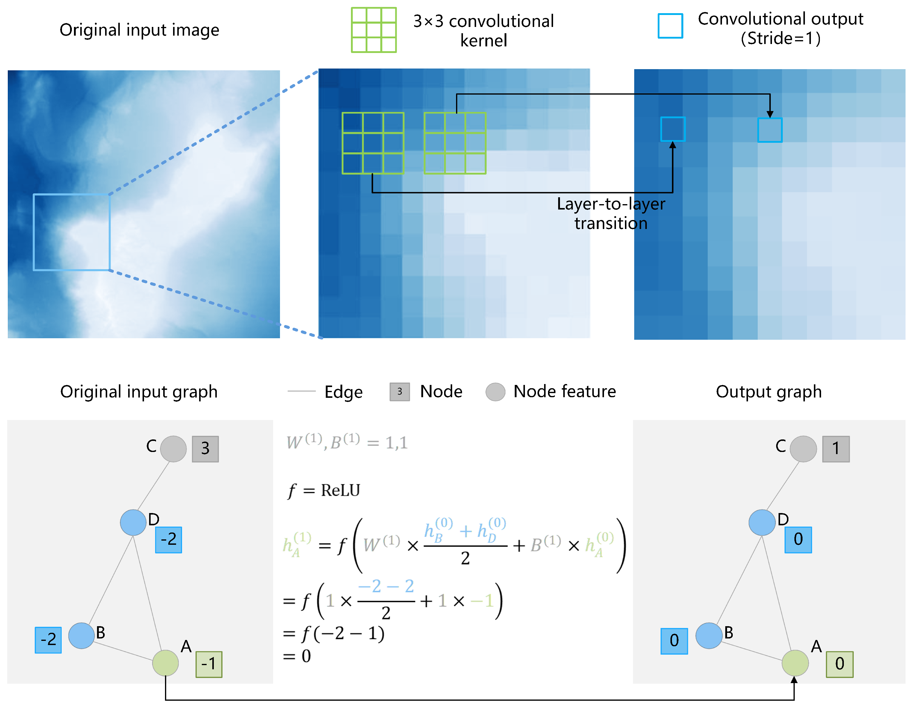
CNN can be viewed as a special form of GNN. In this analogy, each pixel in an image can be regarded as a node in a fixed-structure graph, while the convolution kernel corresponds to a weighted connection between nodes. CNN aggregates neighborhood information by performing weighted summation with a convolutional kernel with translation invariance. This is similar to the message passing mechanism of GNN. Figure 14 illustrates the convolutional operations of GNN and CNN.
The difference is that CNN focuses on information extraction at the pixel feature level, while GNN has an extra neighborhood. The extra dimension of information tends to improve the structural performance of the model. CNN is well suited for processing regular inputs like remote sensing images. However, its convolutional kernel is limited to the local receptive field, which restricts the model’s ability to capture a wider range of contextual information and results in the loss of details. In contrast, GNN addresses this limitation by incorporating spatial relationships into the graph structure or facilitating the exchange of information between distant neighbors.
Unlike the image element matrix structure of image data, map data are not stored in a regular matrix form [158]. Therefore, when dealing with this type of data, it is difficult for traditional CNN to adequately capture their intrinsic structural relationships. GNN effectively models the spatial and topological structures among features through the relationships between nodes and edges, which gives GNN an obvious advantage in cartographic generalization.
GCN performs well in node classification problems through approximated and normalized graph Laplace matrices [137]. The training samples need to have the desired output [159]. Large-scale maps can be used as inputs to the network and corresponding small-scale maps as outputs. Referring to map generalization, see [160,161]. Figure 15 shows the stages of the selection process of soundings based on GNN. Taking the GCN network architecture as an example, soundings selection can be regarded as a binary classification problem of points, and data preprocessing is first performed based on the Delaunay triangular network to construct the graph structure. Then, the features of spatial, contextual, and attribute features are extracted by the Graph Convolution operation. They were mapped in Hidden Layers, which are nonlinearly transformed using activation functions such as Rectified Linear Unit (ReLU). At last, the classification and output are performed through Fully-Connected layers.

5.3. Experimental Verification

The experiment focuses on the generalization of coastlines between large-scale and small-scale electronic nautical charts, modeling the task as a node classification problem using a Graph Neural Network to determine whether a node should be retained or merged. Features from the large-scale chart are used as input, while the small-scale chart serves as the target. A dedicated graph construction strategy is designed to enable the model to learn the underlying simplification patterns of the coastline.

5.3.1. Establishment of a Simple Graph Structure

In this experiment, DBM data of the Guam region are used as the depth background field. Line features—taking the coastline (COALNE field) as an example—are extracted from both large-scale and small-scale nautical charts to generate masks. A buffer zone of a certain width is then created around the masked area to capture spatial neighborhood information effectively.
A simple and intuitive undirected graph structure was established. Specifically, the nodes represent all valid water depth points within the buffer zone, including pixels marked as coastlines in the mask and background points within the buffer zone. The node feature dimension is 3, containing longitude, latitude, and water depth information, i.e., point (lon, lat, depth). In the graph structure representation of the coastline, edges can represent the spatial relationship between adjacent nodes. In the experiment, the feature dimension of the edges was 1. This simple design helps reduce computational complexity while maintaining model efficiency.
The left side of Figure 16 shows the established graph structure, which intuitively illustrates the spatial distribution of nodes of different categories. Category 0 represents background nodes, categories 1 and 2 represent nodes that exist only in large- and small-scale maps, respectively, and category 3 represents consensus nodes that exist in both scales. The histogram on the right clearly describes the distribution of label categories in the graph.

5.3.2. Simple Model Settings

The study adopted a node classification method based on graph convolutional networks (GCNs) to achieve accurate classification of nodes in multi-scale nautical chart data. The model input consists of the spatial features of nodes, namely geographic longitude (lon), latitude (lat), and water depth values (depth).
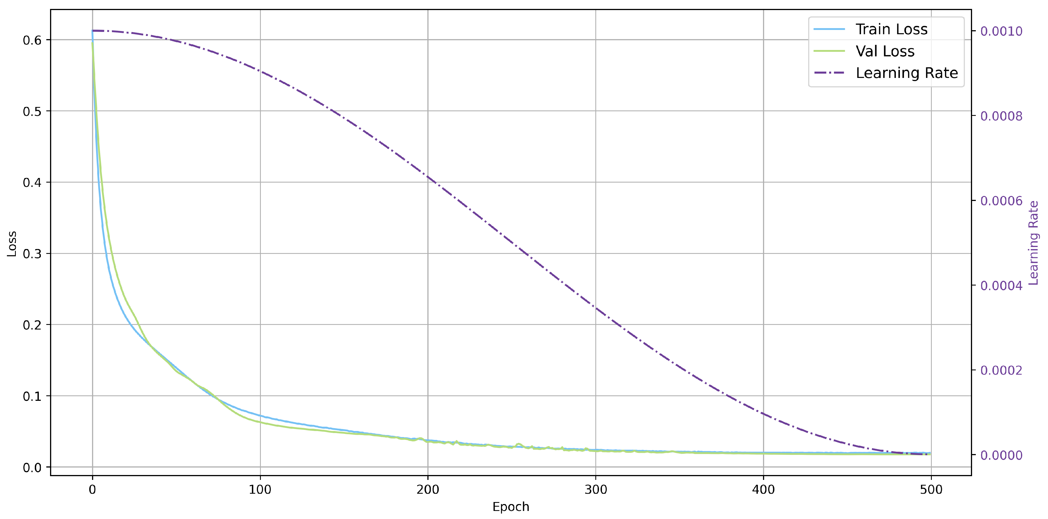
A simple stacked deep Graph Neural Network model with six graph convolutional layers was constructed, expanding the node feature dimension from the initial 3 dimensions to 64 dimensions. Batch normalization (Batch Normalization) was added after each convolutional layer to enhance the stability of the training process. The model ultimately outputs a single-dimensional logit through a fully connected classifier for node classification tasks. BCE, specifically designed for binary classification tasks, was selected as the loss function. The learning rate was dynamically adjusted using the Cosine Annealing strategy, with an initial learning rate of 0.001 and weight decay of 0.001.
Figure 17 shows the trend of the loss function and learning rate during model training and validation. On the whole, the training loss and validation loss decreased significantly within the first 100 rounds, and they then leveled off and converged to an extremely low level after approximately 400 rounds. The model has been fully trained and shows no obvious signs of overfitting. In addition, a learning rate scheduler based on cosine annealing was used to dynamically adjust the learning rate during training. The learning rate gradually decays, which effectively promotes convergence and enhances the model’s generalization ability. In summary, this experiment validates that under the parameter settings and scheduling strategy of a simple GNN, the model exhibits good convergence and robustness, providing a basis for the subsequent performance evaluation and model generalization.
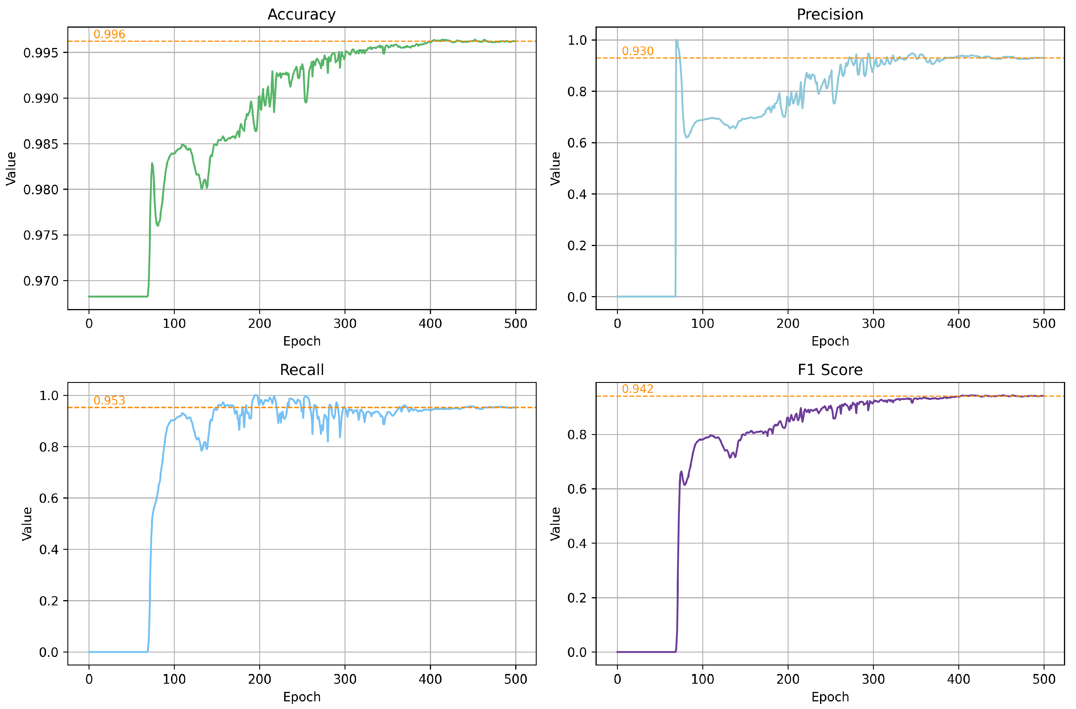
To more accurately evaluate the model training results, multiple metrics such as accuracy, recall, precision, and F1 score were used to summarize the model’s performance, as shown in Figure 18. The accuracy rate ultimately stabilized around 0.995, enabling correct classification of the vast majority of samples. The precision rate stabilized above 0.90, demonstrating the model’s excellent performance in reducing false positives. The recall rate stabilized above 0.90, effectively controlling missed detections. The F1 score stabilized around 0.90 in the later stages of training with minimal fluctuations, indicating that the model achieved a good balance between precision and completeness.
It is worth noting that despite the use of a relatively simple model structure with only basic graph convolution layers stacking and a simple fully connected classifier, without explicit attention mechanisms or complex edge feature modeling. The model can accurately identify different types of nodes in multi-scale seabed map data. This fully demonstrates that the GNN architecture has the advantage of adapting to spatial topology, can effectively use the adjacency relationship between nodes for context information modeling, and has the potential for application in seafloor topography generalization.

5.3.3. Comparison with Traditional Methods

Inference is performed based on the optimal weights saved in the model, and the inference results are visualized. Large-scale coastline data are set as Band 2, representing high-precision, detailed reference data; small-scale target data are set as Band 3, representing the simplified results required for actual traditional cartographic generalization; and model inference output is set as Band 4, representing the automatic generalization results generated by GNN based on multi-scale learning. The spatial distribution of different colors reflects the overlap, differences, and simplification effects between large-scale data, small-scale target data, and inference results, as shown in Figure 19.
Based on the main rules of coastline generalization, the results were analyzed, and the constructed model showed strong structural recognition ability and morphological expression effects in multi-scale coastline generalization. The main coastline area is mainly green (indicating that Bands 2, 3, and 4 are consistent), with high consistency between scales, especially concentrated on key skeletal locations such as turning points and capes, indicating that the model can accurately maintain the location of turning points and satisfy the principle of turning point accuracy. Additionally, the widespread distribution of green and yellow (overlap between Band 2 and Band 3) along the main coastal sections reflects the consistency between the model and actual small-scale nautical charts in terms of shape and direction. Red (Band 2 only) and orange (Band 3 and Band 4 overlap) discontinuities appear only in localized small bays and densely curved areas, indicating that the model reasonably compresses details while retaining the main contours, demonstrating excellent shape retention capability. In terms of adhering to the “expand land, contract sea” principle, it also demonstrates spatial selectivity consistent with cartographic standards. Important promontory protrusions are mostly green, indicating that the inference model has strong retention capability for key topographic structures. Small, concave bays are often only present in large-scale data (red) and are merged and smoothed in small-scale maps and model results correspondingly, thereby achieving the objection.
Compared with traditional generalization methods, the model shows stronger adaptability in terms of structure preservation and shape recognition. It can extract and preserve the main contour structure in multi-scale data while recognizing important local morphological features. In complex coastline areas, the inference results are more consistent, demonstrating superior shape retention and skeleton recognition capabilities, providing more practical technical support for the automation of large-scale nautical chart generalization.

5.4. Challenges

(1) Arithmetic bottlenecks and resource constraints: The storage and computation requirements of multi-source submarine terrain data are exceptionally huge, far exceeding the load capacity of traditional data processing. Although the existing high-performance computing framework GPU acceleration has achieved significant optimization in processing raster data, there are still certain deficiencies in the processing of graph structure data. This makes the arithmetic bottleneck a non-negligible problem in the process of graph data processing, especially when using GNN for deep learning training.
(2) Result assessment and interpretability: The existing system of generalization assessment of nautical charts lacks uniform and systematic quantitative standards [162]. With the application of machine learning in the field of map generalization, traditional map generalization assessment methods face new challenges [163]. Currently, the quality assessment nautical charts primarily relies on empirical qualitative analysis, with a lack of quantitative evaluation. It follows that quality assessment metrics such as reduced depth area and the curvature of depth contours with smooth deviation can be defined.
The problem of network interpretability is also a major challenge in nautical chart generalization in the wide application of deep learning models. Earlier, there were studies on improving the transparency of the generalization process through decision trees [164]. Although GNN performs well in many tasks, their “black-box” nature makes the model’s decision-making process difficult to understand. Fu et al. [165] introduced Explainable Artificial Intelligence (XAI) to map generalization, demonstrating that deep learning methods are capable of learning human-interpretable cartographic knowledge. GeoXAI is able to provide a deeper understanding of complex mechanisms from a data-driven perspective [166]. Therefore, how to improve the interpretability of the model and establish a scientific, comprehensive, and quantitative evaluation system to effectively assess the quality of the generalization results are important challenges in current research.
(3) Data quality, safety, and updating: High-quality marine geospatial data have a dual value as follows: on the one hand, they are directly related to the safety of ship navigation; and on the other hand, they can also provide important data support for marine environmental monitoring and geologic disaster early warning [167]. However, in the application practice of deep learning, data quality often becomes a key bottleneck that restricts the model performance. Most of the current research overly focuses on the optimization of network architecture, but it relatively neglects the enhancement and improvement of dataset quality. There may be large differences in the format, quality, and accuracy of chart data from different sources. The heterogeneity of data brings great challenges to the generalization of nautical charts. How to efficiently handle these heterogeneous data and ensure the consistency and accuracy of the generalization results are some of the present difficulties.
At the same time, nautical chart data involve sensitive information. In order to protect the security of data, the confidentiality and privacy of the chart data need special attention. Therefore, there may be conflicts between data sharing and model training.
Seafloor geomorphology data are dynamically changing. Traditional Graph Neural Network architectures have limited support for dynamic maps, especially when real-time data updates are involved. The development of GNN models that can flexibly cope with dynamic graph changes, especially in efficiently handling incremental graph structures, is one of the key tasks in current research.
(4) Standardization: Nautical charts are an indispensable tool for the safety of maritime navigation. Although the current International Hydrographic Organization has established standard frameworks such as S-57, S-63, and S-101 in data transmission and exchange, there is still a lack of unified technical standards in the field of nautical chart generalization, especially in the intelligent generalization method based on Graph Neural Network. The establishment of a GNN-based generalization standard for nautical charts can not only fill the gaps in the existing standard system, but it may also provide an innovative technical reference framework for international nautical chart standardization [168]. Thus, it can promote the in-depth sharing and application consistency of nautical chart data on a global scale and finally build an intelligent navigation security system that meets the needs of modern shipping.
(5) Ethical risks and algorithmic biases: Artificial intelligence methods such as GNN are increasingly being used. However, in security-sensitive scenarios such as chart generalization, ethical concerns and algorithmic biases may arise. Outdated or unrepresentative training data, as well as incomplete historical data, can bias the model by oversimplifying certain areas or omitting critical information. Moreover, the black-box nature may reduce the interpretability and traceability of the model. This may have an impact on the transparency and accountability of the decision-making process for cartographic synthesis. Therefore, future work needs to emphasize fairness, promote the use of Explainable Artificial Intelligence (XAI) methods, and increase human supervision.

6. Conclusions

This paper provides a comprehensive review of the cartographic operators, traditional methods, and their specific performance in the generalization of soundings, depth contours, coastlines, islands, and reefs. We also conclude that Graph Neural Network in chart generalization shows a strong potential to better capture geographic features, optimize data processing, and automate the generalization process. A preliminary exploration and experimental validation of the multi-scale generalization of the coastline have been carried out. The experimental results show that the proposed GNN has been able to achieve stable and excellent performance while keeping the structure simple, which verifies its feasibility and application value in the generalization of nautical charts. More complex model structures, such as the attention mechanism, complex edge-weight modeling, and more diversified parameters can be further introduced in the follow-up work to enhance the model’s ability to express the complex submarine terrain. This provides an important opportunity for the intelligent development. In the future, the research will further focus on the in-depth application of Geospatial Artificial Intelligence to promote the widespread practice and application of efficient and accurate automated generalization solutions in the fields of geographic information science and cartography. In addition, we acknowledge that AI-driven generalization may introduce potential biases due to data imbalance and model opacity. Future efforts should emphasize fairness, interpretability, and ethical safeguards when applying GNN to critical applications such as nautical chart generalization.

Author Contributions

Conceptualization, Taoning Dong, Anmin Zhang, and Ruifu Wang; methodology, Taoning Dong, Anmin Zhang, and Ruifu Wang; software, Pengxv Chen; validation, Pengxv Chen and Chenyue Sun; formal analysis, Taoning Dong; investigation, Pengxv Chen; writing—original draft preparation, Taoning Dong; writing—review and editing, Ruifu Wang and Anmin Zhang; visualization, Chenyue Sun; supervision, Jiayi Liu; project administration, Chaohua Gan; funding acquisition, Anmin Zhang. All authors have read and agreed to the published version of the manuscript.

Funding

This research was funded by the Key Laboratory of Ocean Geomatics, Ministry of Natural Resources, China, grant number 2024B11.

Data Availability Statement

The raw data supporting the conclusions of this article will be made available by the authors on request.

Conflicts of Interest

The authors declare no conflicts of interest.

References

  1. Hongbo, C.; Wenxuan, F.U.; Mengya, C. A Brief Analysis on the Data Differences between Topographic Map and Electronic Chart. Geomat. Spat. Inf. Technol. 2018, 41, 243–245. [Google Scholar]
  2. Zhao, W.; Hui, Z.; Center, T.H. Reviewon Nautical Chart Automatic Generalization. Hydrogr. Surv. Charting 2017, 37, 51–54. [Google Scholar]
  3. Brassel, K.E.; Weibel, R. A review and conceptual framework of automated map generalization. Int. J. Geogr. Inf. Syst. 1988, 2, 229–244. [Google Scholar] [CrossRef]
  4. Oraas, S. Automated sounding selection. In The International Hydrographic Review; Oxford University Press: Oxford, UK, 1975. [Google Scholar]
  5. Tsoulos, L.; Stefanakis, K. Sounding selection for nautical charts: An expert system approach. In Proceedings of the 18th International Cartographic Conference, Stockholm, Sweden, 23–27 June 1997; pp. 23–27. [Google Scholar]
  6. Nada, T.; Kastrisios, C.; Calder, B.; Ence, C.; Greene, C.; Bethell, A. Towards automating the nautical chart generalization workflow. Geo-Spat. Inf. Sci. 2024, 27, 1–26. [Google Scholar] [CrossRef]
  7. Woodlief, M. Unlock insights from hydrographic data with GeoAI. Int. Hydrogr. Rev 2024, 30, 144–149. [Google Scholar] [CrossRef]
  8. Wang, J.Y.; Tian, Z. The cartographic generalization of soundings on chart by artificial neural network techniques. Acta Geod. Cartogr. Sin. 1999, 28, 335–339. [Google Scholar]
  9. Jia, S.; Song, Z.; Zhang, L.; Liang, Z. A Case-Based Reasoning Method for Generalizing Depth Contours considering Both Navigational Safety Assurance and Line Shape Preservation. Mar. Geod. 2024, 47, 1–22. [Google Scholar] [CrossRef]
  10. Song, Z.; Jia, S.; Liang, Z.; Zhang, L.; Liang, C. A reinforcement learning method for collaborative generalization of soundings and depth contours. Acta Geod. Cartogr. Sin. 2024, 53, 1345. [Google Scholar]
  11. Wu, F.; Du, J.; Qian, H.; Zhai, R. Overview of research progress and reflections in intelligent map generalization. Geomat. Inf. Sci. Wuhan Univ. 2022, 47, 1675–1687. [Google Scholar]
  12. Yu, W. Automatic sounding generalization in nautical chart considering bathymetry complexity variations. Mar. Geod. 2018, 41, 68–85. [Google Scholar] [CrossRef]
  13. Lu, Y.; Zhai, J.; Du, J. Sounding selection based on recognition of submarine topography features. J. Inst. Surv. Mapp. 2000, 17, 296–300. [Google Scholar]
  14. Zhai, J.; Lu, Y. Recognition and measurement of marine topography for sounding generalization in digital nautical chart. Mar. Geod. 2005, 28, 167–174. [Google Scholar]
  15. Jinghan, L.I.; Fang, W.U.; Ruixing, X.; Jiawei, D.U.; Qingguang, D.; University, I.E. Recognition of Complex Seabed Regions for Nautical Chart Generalization. J. Geomat. Sci. Technol. 2018, 35, 524–528. [Google Scholar]
  16. Wang, M.; Zhang, L.; Yu, C.; Liu, T. Distilling Feature Shallow Points from Soundings Based on the Slope-Relationship. Geomat. Inf. Sci. Wuhan Univ. 2016, 41, 208–213. [Google Scholar]
  17. Liu, Y.; Zhai, J.; Lu, Y.; Wang, M. Automatic generalization of sounding in digital chart. Acta Geod. et Cartogr. Sin. 2005, 34, 179–184. [Google Scholar]
  18. Li, J. Research on Automated Cartographic Generalization of Submarine Relief. Ph.D. Thesis, PLA Strategic Support Force Information Engineering University, Zhengzhou, China, 2018. [Google Scholar]
  19. Li, J.; Wu, F.; Du, J.; Gong, X.; Xing, R. Chart Depth Contour Simplification Based on Delaunay Triangulation. Geomat. Inf. Sci. Wuhan Univ. 2019, 44, 778–783. [Google Scholar]
  20. Li, J.; Wu, F.; Du, J.; Xing, R. Study on Automated Aggregation of Depth Contour on Nautical Charts. Geomat. Inf. Sci. Wuhan Univ. 2019, 44, 1484–1490. [Google Scholar]
  21. Ai, T.; Zhou, Q.; Zhang, X.; Huang, Y.; Zhou, M. A simplification of ria coastline with geomorphologic characteristics preserved. Mar. Geod. 2014, 37, 167–186. [Google Scholar] [CrossRef]
  22. Tang, L.; Zhang, L.; Dong, J.; Wei, H.; Wei, S. An Adaptive Simplification Method for Coastlines Using a Skeleton Line “Bridge” Double Direction Buffering Algorithm. ISPRS Int. J. Geo-Inf. 2024, 13, 155. [Google Scholar] [CrossRef]
  23. Lu, Y.; Zhai, J.; Du, J.; Li, S. Recognition, measurement and generalization for point cluster features in digital nautical chart. Geomat. Inf. Sci. Wuhan Univ. 2001, 26, 133–139. [Google Scholar]
  24. Huang, Y.; Ai, T.; Liu, Y.; Zhang, H. Geographic-feature oriented ria coastline simplification. Acta Geod. Cartogr. Sin. 2013, 42, 595–601. [Google Scholar]
  25. Huang, Y. Research on Supporting Data Models and Methods for Maritime Feature Generalization; Wuhan University: Wuhan, China, 2011. [Google Scholar]
  26. Yafeng, H.; Tinghua, A.I.; Hangfeng, Z. Automatic selection of soundings based on Voronoi diagram. Sci. Surv. Mapp. 2016, 41, 28–33. [Google Scholar] [CrossRef]
  27. Peters, R.; Ledoux, H.; Meijers, M. A Voronoi-based approach to generating depth-contours for hydrographic charts. Mar. Geod. 2014, 37, 145–166. [Google Scholar] [CrossRef]
  28. Yan, H.; Weibel, R. An algorithm for point cluster generalization based on the Voronoi diagram. Comput. Geosci. 2008, 34, 939–954. [Google Scholar] [CrossRef]
  29. Chen, Z.; Zheng, Y. An Automatic Selecting Model of Islands in Chart. Hydrogr. Surv. Charting 2005, 25, 23–25. [Google Scholar]
  30. Tang, L.; Zhang, L.; Xu, W.; Jia, S.; Dong, J. A Composite Influence Domain Model for Automatically Selecting Islands in Nautical Charts. Mar. Geod. 2020, 43, 189–212. [Google Scholar] [CrossRef]
  31. Zhu, J.; Lu, Y. A New Method of Island Cartography Generalization. Hydrogr. Surv. Charting 2004, 17–19. [Google Scholar]
  32. Fei, L.; He, J. A three-dimensional Douglas–Peucker algorithm and its application to automated generalization of DEMs. Int. J. Geogr. Inf. Sci. 2009, 23, 703–718. [Google Scholar] [CrossRef]
  33. Shuaidong, J.; Lihua, Z.; Rencan, P. Method for automatic selection of water depth harmonizing with a depth contour. J. Harbin Eng. Univ. 2016, 37, 59–64. [Google Scholar]
  34. Guimin, H.; Jinhua, G.; Lin, L. Research on Depth Contour Generalization Method Based on Curve Characteristic. Hydrogr. Surv. Charting 2014, 34, 38–41. [Google Scholar]
  35. Haisen, L.; Dan, L.; Yukuo, W.; Bin, Y. Fast algorithm of contour generation for a multibeam seafloor terrain. J. Harbin Eng. Univ. 2012, 33, 622–628. [Google Scholar]
  36. Yang, H.; Li, L.; Hu, H.; Wu, Y.; Xia, H.; Liu, Y.; Tan, S. A coastline generalization method that considers buffer consistency. PLoS ONE 2018, 13, e0206565. [Google Scholar] [CrossRef] [PubMed]
  37. Qi, Q.; Liu, Y. An Automated Solution to the Graphic Generalization of Discontinuous Area Phenomena. Geogr. Res. 1996, 15, 1–10. [Google Scholar]
  38. Sui, H.; Zhu, X.; Zhang, A. A system for fast cartographic sounding selection. Mar. Geod. 2005, 28, 159–165. [Google Scholar] [CrossRef]
  39. Tang, L.; Zhang, L.; Jia, S. A method for selecting islands based on their influence domains. Hydrogr. Surv. Charting 2018, 38, 67–70. [Google Scholar]
  40. Tang, L.; Zhang, L.; Jia, S.; Li, B. A Method for Islands Automatic Selection Based on Buffer Dynamic Growing Model. Geomat. Inf. Sci. Wuhan Univ. 2019, 44, 1874–1882. [Google Scholar]
  41. Tang, L.; Zhang, L.; Jia, S.; Liu, X. Line Element Synthesis Method Based on Rolling-circle. Hydrogr. Surv. Charting 2019, 39, 16–19. [Google Scholar]
  42. Tang, L.; Zhang, L.; Dong, J.; Jia, S. Automatic simplification and merging algorithm of isobaths based on surface simplification. In Proceedings of the International Conference on Geographic Information and Remote Sensing Technology (GIRST 2022), Kunming, China, 16–18 September 2022; Volume 12552, pp. 898–903. [Google Scholar]
  43. Guilbert, E.; Saux, E. Cartographic generalisation of lines based on a B-spline snake model. Int. J. Geogr. Inf. Sci. 2008, 22, 847–870. [Google Scholar] [CrossRef]
  44. Miao, D. Gradual Generalization of Nautical Chart Contours with a B-Spline Snake Method. Master’s Thesis, University of New Hampshire, Durham, NH, USA, 2014. [Google Scholar]
  45. Miao, D.; Calder, B. Gradual generalization of nautical chart contours with a cubic B-spline snake model. In Proceedings of the 2013 OCEANS-San Diego, San Diego, CA, USA, 23–27 September 2013; pp. 1–7. [Google Scholar]
  46. Wu, F.; Zhu, K. Geometric accuracy assessment of linear features’ simplification algorithms. Geomat. Inf. Sci. Wuhan Univ. 2008, 33, 600–603. [Google Scholar]
  47. Fang, W.; Jiawei, D.; Fanghua, W. A survey of the research progress in automated generalization of submarine terrain data. Acta Geod. Cartogr. Sin. 2022, 51, 1588. [Google Scholar]
  48. Tang, Q. A study on automated generalization of submarine relief. Acta Geod. Cartogr. Sin. 1987, 16, 314–320. [Google Scholar]
  49. Zhu, M.; Yang, B.; Wang, M.; You, B.; Liu, G. The present situation and analysis of the comprehensive study of water depth in digital chart. Hydrogr. Surv. Charting 2018, 38, 11. [Google Scholar]
  50. Zoraster, S.; Bayer, S. Automated cartographic sounding selection. Int. Hydrogr. Rev. 1992, 69, 57–61. [Google Scholar]
  51. Dyer, N.; Kastrisios, C.; De Floriani, L. Label-based generalization of bathymetry data for hydrographic sounding selection. Cartogr. Geogr. Inf. Sci. 2022, 49, 338–353. [Google Scholar] [CrossRef]
  52. Dyer, N.; Kastrisios, C.; De Floriani, L. Chart features, data quality, and scale in cartographic sounding selection from composite bathymetric data. Geo-Spat. Inf. Sci. 2024, 27, 1542–1567. [Google Scholar] [CrossRef]
  53. Stateczny, A.; Gronska-Sledz, D.; Motyl, W. Precise bathymetry as a step towards producing bathymetric electronic navigational charts for comparative (terrain reference) navigation. J. Navig. 2019, 72, 1623–1632. [Google Scholar] [CrossRef]
  54. Smith, S.M.; Alexander, L.; Armstrong, A.A. The navigation surface: A new database approach to creating multiple products from high-density surveys. Int. Hydrogr. Rev. 2002, 3, 12–16. [Google Scholar]
  55. Maleika, W. The Effect of the Density of Measurement Points Collected from a Multibeam Echosounder on the Selection of IDW Interpolation Points in the Process of Creating Seabed Models. IEEE J. Sel. Top. Appl. Earth Obs. Remote Sens. 2024, 17, 7292–7304. [Google Scholar] [CrossRef]
  56. Wen, J.; Li, J.; Xing, R.; Du, J.; Liu, X. A thinning algorithm of multibeam sounding data considering the complexity of seabed terrain. J. Geomat. Sci. Technol. 2018, 35, 435–440. [Google Scholar]
  57. Mo, W.; He-Yuan, L.I.; Xiao-Nan, Z. A sounding-generalization method based on the rhomb box-counting fractal dimension estimate. Eng. Surv. Mapp. 2015, 24, 17–21. [Google Scholar] [CrossRef]
  58. Skopeliti, A.; Stamou, L.; Tsoulos, L.; Pe’eri, S. Generalization of soundings across scales: From DTM to harbour and approach nautical charts. ISPRS Int. J. Geo-Inf. 2020, 9, 693. [Google Scholar] [CrossRef]
  59. Li, M.; Zhang, A.; Zhang, D.; Di, M.; Liu, Q. Automatic Sounding Generalization Maintaining the Characteristics of Submarine Topography. IEEE J. Sel. Top. Appl. Earth Obs. Remote Sens. 2021, 14, 10278–10286. [Google Scholar] [CrossRef]
  60. Yu, L.; Du, J.; Zhai, R.; Wu, F.; Qian, H. A fast generalization method of multibeam echo soundings for nautical charting. J. Geovis. Spat. Anal. 2022, 6, 1–12. [Google Scholar] [CrossRef]
  61. Tsai, V.J. Delaunay triangulations in TIN creation: An overview and a linear-time algorithm. Int. J. Geogr. Inf. Sci. 1993, 7, 501–524. [Google Scholar] [CrossRef]
  62. Ying, Z.; Yi, L.U.; Hong-Yan, J.; Ming, S.; Zhong-Dong, Z.; Ying, C.; Yan, L.U. Research on Automatic Generalization of Digital Soundings. Hydrogr. Surv. Charting 2008, 48–51. [Google Scholar]
  63. Kastrisios, C.; Calder, B.; Masetti, G.; Holmberg, P. Towards automated validation of charted soundings: Existing tests and limitations. Geo-Spat. Inf. Sci. 2019, 22, 290–303. [Google Scholar] [CrossRef]
  64. Zhang, L.; Jia, S.; Wu, C.; Yin, X. A method for interpolating digital depth model considering uncertainty. Acta Geod. Cartogr. Sin. 2011, 40, 359–365. [Google Scholar]
  65. Jia, S.; Zhang, L.; Dong, J.; Peng, R. A method for constructing DDM serving for navigation using pre-constructed model surface to control and adjust the selection of DDM nodes. Geomat. Inf. Sci. Wuhan Univ. 2019, 44, 1715–1722. [Google Scholar]
  66. Alcaras, E.; Amoroso, P.P.; Figliomeni, F.G.; Parente, C.; Vallario, A. Using Electronic Navigational Chart for 3D bathymetric model of the port of Naples. Int. Arch. Photogramm. Remote Sens. Spat. Inf. Sci. 2023, 48, 7–13. [Google Scholar] [CrossRef]
  67. Guilbert, E.; Zhang, X. Generalisation of submarine features on nautical charts. ISPRS Ann. Photogramm. Remote Sens. Spat. Inf. Sci. 2012, 1, 13–18. [Google Scholar] [CrossRef]
  68. Saux, E. B-spline functions and wavelets for cartographic line generalization. Cartogr. Geogr. Inf. Sci. 2003, 30, 33–50. [Google Scholar] [CrossRef]
  69. Xing, R.; Wu, F.; Li, J.; Gong, X. A fast algorithm of contour generation considering ambiguity. J. Comput.-Aided Des. Comput. Graph. 2017, 29, 1705–1712. [Google Scholar]
  70. Lida, W.; Xiaodong, Y.; Lihua, Z. Efficient Algorithm to Tracing Nodes of Equivalent Depth Based on Topology of Triangles. Port Waterw. Eng. 2007, 13–16. [Google Scholar]
  71. Wang, Z.; Müller, J.C. Line generalization based on analysis of shape characteristics. Cartogr. Geogr. Inf. Syst. 1998, 25, 3–15. [Google Scholar] [CrossRef]
  72. Hongcheng, W.; Lihua, Z.; Lulu, T.; Jian, D.; Gaixiao, L.; Hao, Y. Complexity measurement of line element on nautical chart considering local difference. Acta Geod. Cartogr. Sin. 2022, 51, 1959. [Google Scholar]
  73. Li, J.; Wu, F.; Gong, X.; Du, J.; Xing, R. Depth contour smoothing based on the fitting of multi-segment bezier curves. Mar. Geod. 2018, 41, 382–404. [Google Scholar] [CrossRef]
  74. Lianfa, W.; Lihua, Z.; Shuaidong, J. Application of Snake Model in Auto Simplification of a Depth-Contour. Hydrogr. Surv. Charting 2016, 36, 15–18. [Google Scholar]
  75. Kim, Y.J.; Lee, J.S.; Kong, G.Y.; Cho, I.S. A study on the creation of high density depth contours in coastal waters using spatial analysis based on depth and AIS data. J. Coast. Disaster Prev. 2022, 9, 157–165. [Google Scholar] [CrossRef]
  76. Skopeliti, A.; Tsoulos, L.; Pe’eri, S. Depth contours and coastline generalization for harbour and approach nautical charts. ISPRS Int. J. Geo-Inf. 2021, 10, 197. [Google Scholar] [CrossRef]
  77. Ning, Z.; Jiang, C.; Chen, J.; Wu, Z.; Yao, Z.; Ma, Y.; Deng, T.; Chen, Y. Long-term spatiotemporal analysis of coastline morphological evolutions and their underlying mechanisms in the Pearl River Delta region of China. Ocean Coast. Manag. 2024, 258, 107426. [Google Scholar] [CrossRef]
  78. Liu, H.; Xie, S.; Wang, F. Study on the Method of Automatic Cartographic Generalization of Coastline. J. Geomat. Sci. Technol 2010, 27, 225–228. [Google Scholar]
  79. Christensen, A.H. Cartographic line generalization with waterlines and medial-axes. Cartogr. Geogr. Inf. Sci. 1999, 26, 19–32. [Google Scholar] [CrossRef]
  80. Lewin, S.; Jiang, X.; Clausing, A. Perceptually motivated shape evolution with shape-preserving property. Pattern Recognit. Lett. 2010, 31, 447–453. [Google Scholar] [CrossRef]
  81. Visvalingam, M.; Whyatt, J.D. Line generalization by repeated elimination of points. In Landmarks in Mapping; Routledge: London, UK, 2017; pp. 144–155. [Google Scholar]
  82. Chen, H.; Peng, R.; Zheng, Y.; Li, S. Coastline generalization based on skeleton line of curve bends. Geomat. Inf. Sci. Wuhan Univ. 2011, 36, 1418–1422. [Google Scholar]
  83. Ai, T. The drainage network extraction from contour lines for contour line generalization. ISPRS J. Photogramm. Remote Sens. 2007, 62, 93–103. [Google Scholar] [CrossRef]
  84. Liu, Y.; Zhai, J. The research on pattern presentation and automatic generalization of coastlines. Geomat. Spat. Inf. Technol 2005, 28, 78–81. [Google Scholar]
  85. Wang, L.; Wu, Y.; Tang, J. A coastline generalization method for marine delimitation. Sci. Surv. Mapp 2015, 40, 18–21. [Google Scholar] [CrossRef]
  86. Töpfer, F.; Pillewizer, W. The principles of selection. Cartogr. J. 1966, 3, 10–16. [Google Scholar] [CrossRef]
  87. Steiniger, S.; Burghardt, D.; Weibel, R. Recognition of island structures for map generalization. In Proceedings of the 14th Annual ACM International Symposium on Advances in Geographic Information Systems, Hamburg, Germany, 13–16 November 2006; pp. 67–74. [Google Scholar]
  88. Anderson-Tarver, C.; Leyk, S.; Buttenfield, B.P. Fuzzy modeling of geometric textures for identifying archipelagos in area-patch generalization. Cartogr. Geogr. Inf. Sci. 2011, 38, 137–145. [Google Scholar] [CrossRef]
  89. Müller, J.; Zeshen, W. Area-patch generalisation: A competitive approach. Cartogr. J. 1992, 29, 137–144. [Google Scholar] [CrossRef]
  90. Qiao, W.; Hehai, W. The research on fractal method of automatic generalization of map polygons. Geomat. Inf. Sci. Wuhan Univ. 1996, 21, 59–63. [Google Scholar]
  91. McBrearty, I.W.; Beroza, G.C. Earthquake location and magnitude estimation with graph neural networks. In Proceedings of the IEEE International Conference on Image Processing (ICIP), Bordeaux, France, 16–19 October 2022; pp. 3858–3862. [Google Scholar]
  92. Zhang, F.; Sun, Q.; Huang, W.; Su, Y.; Ma, J.; Xing, R. Enhancing the Recognition of Collinear Building Patterns by Shape Cognition Based on Graph Neural Networks. Appl. Artif. Intell. 2024, 38, 2439611. [Google Scholar] [CrossRef]
  93. Rampášek, L.; Galkin, M.; Dwivedi, V.P.; Luu, A.T.; Wolf, G.; Beaini, D. Recipe for a general, powerful, scalable graph transformer. Adv. Neural Inf. Process. Syst. 2022, 35, 14501–14515. [Google Scholar]
  94. Shi, Y.; Li, Q.; Zhu, X.X. Building segmentation through a gated graph convolutional neural network with deep structured feature embedding. ISPRS J. Photogramm. Remote Sens. 2020, 159, 184–197. [Google Scholar] [CrossRef]
  95. Pan, Z.; Xu, L.; Chen, N. Combining graph neural network and convolutional LSTM network for multistep soil moisture spatiotemporal prediction. J. Hydrol. 2025, 651, 132572. [Google Scholar] [CrossRef]
  96. Yu, D.; Bai, G.; Li, Y.; Zhao, L. Deep spatial domain generalization. In Proceedings of the IEEE International Conference on Data Mining (ICDM), Orlando, FL, USA, 28 November–1 December 2022; pp. 1293–1298. [Google Scholar]
  97. Li, Y.; Lu, X.; Yan, H.; Wang, W.; Li, P. A skeleton-line-based graph convolutional neural network for areal settlements’ shape classification. Appl. Sci. 2022, 12, 10001. [Google Scholar] [CrossRef]
  98. Tianyuan, X.; Tinghua, A.; Huafei, Y.; Min, Y.; Pengcheng, L. A point cluster simplification approach of graph convolutional neural network for map generalization. Acta Geod. Cartogr. Sin. 2024, 53, 158. [Google Scholar]
  99. Wang, X.; Girshick, R.; Gupta, A.; He, K. Non-local neural networks. In Proceedings of the IEEE Conference on Computer Vision and Pattern Recognition, Salt Lake City, UT, USA, 18–22 June 2018; pp. 7794–7803. [Google Scholar]
  100. Li, W.; Fu, Y.; Fan, S.; Xin, M.; Bai, H. DCI-PGCN: Dual-channel interaction portable graph convolutional network for landslide detection. IEEE Trans. Geosci. Remote Sens. 2023, 61, 1–16. [Google Scholar] [CrossRef]
  101. Zheng, H.; Zhang, J.; Li, H.; Wang, G.; Guo, J.; Wang, J. Road Network Intelligent Selection Method Based on Heterogeneous Graph Attention Neural Network. ISPRS Int. J. Geo-Inf. 2024, 13, 300. [Google Scholar] [CrossRef]
  102. Wang, T.; Li, Z.; Geng, X.; Jin, B.; Xu, L. Time series prediction of sea surface temperature based on an adaptive graph learning neural model. Future Internet 2022, 14, 171. [Google Scholar] [CrossRef]
  103. Gao, Z.; Li, Z.; Yu, J.; Xu, L. Global spatiotemporal graph attention network for sea surface temperature prediction. IEEE Geosci. Remote Sens. Lett. 2023, 20, 1–5. [Google Scholar] [CrossRef]
  104. Haigang, S.; Penggen, C.; Anming, Z.; Jianya, G. An algorithm for automatic cartographic sounding selection. Geo-Spat. Inf. Sci. 1999, 2, 96–99. [Google Scholar] [CrossRef]
  105. He, L.; Nan, J.; Chen, L.; Ye, X.; Ji, S.; Chen, Z.; Zhang, Y.; Wu, F.; Liu, B.; Ge, Z.; et al. Spatiotemporal graph convolutional network using sparse monitoring data for accurate water-level reconstruction in urban drainage systems. J. Hydrol. 2025, 652, 132681. [Google Scholar] [CrossRef]
  106. Shi, Z.; Liang, X.; Wang, J. LMC: Fast training of GNNs via subgraph sampling with provable convergence. arXiv 2023, arXiv:2302.00924. [Google Scholar]
  107. Chiang, W.L.; Liu, X.; Si, S.; Li, Y.; Bengio, S.; Hsieh, C.J. Cluster-gcn: An efficient algorithm for training deep and large graph convolutional networks. In Proceedings of the 25th ACM SIGKDD International Conference on Knowledge Discovery & Data Mining, Anchorage, AK, USA, 4–8 August 2019; pp. 257–266. [Google Scholar]
  108. Elmore, P.; Calder, B.; Petry, F.; Masetti, G.; Yager, R. Aggregation Methods Using Bathymetry Sources of Differing Subjective Reliabilities for Navigation Mapping. Mar. Geod. 2023, 46, 99–128. [Google Scholar] [CrossRef]
  109. Zeng, H.; Zhu, Q.; Ding, Y.; Hu, H.; Chen, L.; Xie, X.; Chen, M.; Yao, Y. Graph neural networks with constraints of environmental consistency for landslide susceptibility evaluation. Int. J. Geogr. Inf. Sci. 2022, 36, 2270–2295. [Google Scholar] [CrossRef]
  110. Shi, N.; Xu, J.; Wurster, S.W.; Guo, H.; Woodring, J.; Van Roekel, L.P.; Shen, H.W. Gnn-surrogate: A hierarchical and adaptive graph neural network for parameter space exploration of unstructured-mesh ocean simulations. IEEE Trans. Vis. Comput. Graph. 2022, 28, 2301–2313. [Google Scholar] [CrossRef]
  111. Yan, X.; Ai, T.; Yang, M.; Yin, H. A graph convolutional neural network for classification of building patterns using spatial vector data. ISPRS J. Photogramm. Remote Sens. 2019, 150, 259–273. [Google Scholar] [CrossRef]
  112. Yan, X.; Ai, T.; Yang, M.; Tong, X. Graph convolutional autoencoder model for the shape coding and cognition of buildings in maps. Int. J. Geogr. Inf. Sci. 2021, 35, 490–512. [Google Scholar] [CrossRef]
  113. Yangyang, Y.; Kangjie, H.; Fang, W.; Junkui, X. Graph convolution neural network method for shape classification of areal settlements. Acta Geod. Cartogr. Sin. 2022, 51, 2390. [Google Scholar]
  114. Xiao, T.; Ai, T.; Burghardt, D.; Liu, P.; Yang, M.; Gao, A.; Kong, B.; Yu, H. A road generalization method using graph convolutional network based on mesh-line structure unit. Geocarto Int. 2024, 39, 2413549. [Google Scholar] [CrossRef]
  115. Veličković, P.; Cucurull, G.; Casanova, A.; Romero, A.; Lio, P.; Bengio, Y. Graph attention networks. arXiv 2017, arXiv:1710.10903. [Google Scholar]
  116. Hamilton, W.; Ying, Z.; Leskovec, J. Inductive representation learning on large graphs. Adv. Neural Inf. Process. Syst. 2017, 30, 1025–1035. [Google Scholar]
  117. Gilmer, J.; Schoenholz, S.S.; Riley, P.F.; Vinyals, O.; Dahl, G.E. Neural message passing for quantum chemistry. In Proceedings of the International Conference on Machine Learning, Sydney, Australia, 6–11 August 2017; pp. 1263–1272. [Google Scholar]
  118. Du, J.; Zhang, S.; Wu, G.; Moura, J.M.; Kar, S. Topology adaptive graph convolutional networks. arXiv 2017, arXiv:1710.10370. [Google Scholar]
  119. Zhang, H.; He, B.; Xing, J.; Lu, M. Deep spatial and temporal graph convolutional network for rice planthopper population dynamic forecasting. Comput. Electron. Agric. 2023, 210, 107868. [Google Scholar] [CrossRef]
  120. Huang, Z.; Derin, Y.; Kirstetter, P.E.; Li, Y. Multigraph convolutional networks for rainfall estimation in complex terrain. IEEE Geosci. Remote Sens. Lett. 2022, 19, 1506005. [Google Scholar] [CrossRef]
  121. Maurya, S.K.; Liu, X.; Murata, T. Improving graph neural networks with simple architecture design. arXiv 2021, arXiv:2105.07634. [Google Scholar]
  122. Wang, L.; Dai, M.; He, J.; Huang, J. Regularized primitive graph learning for unified vector mapping. In Proceedings of the IEEE/CVF International Conference on Computer Vision, Paris, France, 2–3 October 2023; pp. 16817–16826. [Google Scholar]
  123. Zhou, J.; Cui, G.; Hu, S.; Zhang, Z.; Yang, C.; Liu, Z.; Wang, L.; Li, C.; Sun, M. Graph neural networks: A review of methods and applications. AI Open 2020, 1, 57–81. [Google Scholar] [CrossRef]
  124. Liu, B.; Gao, K.; Yu, A.; Guo, W.; Wang, R.; Zuo, X. Semisupervised graph convolutional network for hyperspectral image classification. J. Appl. Remote Sens. 2020, 14, 026516. [Google Scholar] [CrossRef]
  125. Khodayar, M.; Wang, J. Spatio-temporal graph deep neural network for short-term wind speed forecasting. IEEE Trans. Sustain. Energy 2018, 10, 670–681. [Google Scholar] [CrossRef]
  126. Li, P.; Hao, H.; Zhang, Z.; Mao, X.; Xu, J.; Lv, Y.; Chen, W.; Ge, D. A field study to estimate heavy metal concentrations in a soil-rice system: Application of graph neural networks. Sci. Total Environ. 2022, 832, 155099. [Google Scholar] [CrossRef]
  127. Cachay, S.R.; Erickson, E.; Bucker, A.F.C.; Pokropek, E.; Potosnak, W.; Bire, S.; Osei, S.; Lütjens, B. The World as a Graph: Improving El Ni∖˜ no Forecasts with Graph Neural Networks. arXiv 2021, arXiv:2104.05089. [Google Scholar]
  128. Shi, Y.; Li, Q.; Zhu, X. Building footprint extraction with graph convolutional network. In Proceedings of the IGARSS 2019-2019 IEEE International Geoscience and Remote Sensing Symposium, Yokohama, Japan, 28 July–2 August 2019; pp. 5136–5139. [Google Scholar]
  129. Niu, X.; Qian, H.; Wang, X.; Xie, L.; Cui, L. Determining the optimal generalization operators for building footprints using an improved graph neural network model. Geocarto Int. 2024, 39, 2306265. [Google Scholar] [CrossRef]
  130. Zheng, J.; Gao, Z.; Ma, J.; Shen, J.; Zhang, K. Deep graph convolutional networks for accurate automatic road network selection. ISPRS Int. J. Geo-Inf. 2021, 10, 768. [Google Scholar] [CrossRef]
  131. Karsznia, I.; Sielicka, K. When traditional selection fails: How to improve settlement selection for small-scale maps using machine learning. ISPRS Int. J. Geo-Inf. 2020, 9, 230. [Google Scholar] [CrossRef]
  132. Lam, R.; Sanchez-Gonzalez, A.; Willson, M.; Wirnsberger, P.; Fortunato, M.; Alet, F.; Ravuri, S.; Ewalds, T.; Eaton-Rosen, Z.; Hu, W.; et al. Learning skillful medium-range global weather forecasting. Science 2023, 382, 1416–1421. [Google Scholar] [CrossRef]
  133. Wan, S.; Gong, C.; Zhong, P.; Du, B.; Zhang, L.; Yang, J. Multiscale dynamic graph convolutional network for hyperspectral image classification. IEEE Trans. Geosci. Remote Sens. 2019, 58, 3162–3177. [Google Scholar] [CrossRef]
  134. Dong, Y.; Liu, Q.; Du, B.; Zhang, L. Weighted feature fusion of convolutional neural network and graph attention network for hyperspectral image classification. IEEE Trans. Image Process. 2022, 31, 1559–1572. [Google Scholar] [CrossRef]
  135. Scarselli, F.; Gori, M.; Tsoi, A.C.; Hagenbuchner, M.; Monfardini, G. The graph neural network model. IEEE Trans. Neural Netw. 2008, 20, 61–80. [Google Scholar] [CrossRef]
  136. Bruna, J.; Zaremba, W.; Szlam, A.; LeCun, Y. Spectral networks and locally connected networks on graphs. arXiv 2013, arXiv:1312.6203. [Google Scholar]
  137. Kipf, T.N.; Welling, M. Semi-supervised classification with graph convolutional networks. arXiv 2016, arXiv:1609.02907. [Google Scholar]
  138. Ying, R.; He, R.; Chen, K.; Eksombatchai, P.; Hamilton, W.L.; Leskovec, J. Graph convolutional neural networks for web-scale recommender systems. In Proceedings of the 24th ACM SIGKDD International Conference on Knowledge Discovery & Data Mining, London, UK, 19–23 August 2018; pp. 974–983. [Google Scholar]
  139. Dai, H.; Li, H.; Tian, T.; Huang, X.; Wang, L.; Zhu, J.; Song, L. Adversarial attack on graph structured data. In Proceedings of the International Conference on Machine Learning, Stockholm, Sweden, 10–15 July 2018; pp. 1115–1124. [Google Scholar]
  140. Gasteiger, J.; Weißenberger, S.; Günnemann, S. Diffusion improves graph learning. Adv. Neural Inf. Process. Syst. 2019, 32, 13366–13378. [Google Scholar]
  141. Zhang, C.; Song, D.; Huang, C.; Swami, A.; Chawla, N.V. Heterogeneous graph neural network. In Proceedings of the 25th ACM SIGKDD International Conference on Knowledge Discovery & Data Mining, Anchorage, AK, USA, 4–8 August 2019; pp. 793–803. [Google Scholar]
  142. Manessi, F.; Rozza, A.; Manzo, M. Dynamic graph convolutional networks. Pattern Recognit. 2020, 97, 107000. [Google Scholar] [CrossRef]
  143. Skarding, J.; Gabrys, B.; Musial, K. Foundations and modeling of dynamic networks using dynamic graph neural networks: A survey. IEEE Access 2021, 9, 79143–79168. [Google Scholar] [CrossRef]
  144. Shehzad, A.; Xia, F.; Abid, S.; Peng, C.; Yu, S.; Zhang, D.; Verspoor, K. Graph transformers: A survey. arXiv 2024, arXiv:2407.09777. [Google Scholar]
  145. Yuan, H.; Yu, H.; Gui, S.; Ji, S. Explainability in graph neural networks: A taxonomic survey. IEEE Trans. Pattern Anal. Mach. Intell. 2022, 45, 5782–5799. [Google Scholar] [CrossRef]
  146. Wang, C.; Tsepa, O.; Ma, J.; Wang, B. Graph-mamba: Towards long-range graph sequence modeling with selective state spaces. arXiv 2024, arXiv:2402.00789. [Google Scholar]
  147. Touya, G.; Zhang, X.; Lokhat, I. Is deep learning the new agent for map generalization? Int. J. Cartogr. 2019, 5, 142–157. [Google Scholar] [CrossRef]
  148. Kang, Y.; Gao, S.; Roth, R.E. Artificial intelligence studies in cartography: A review and synthesis of methods, applications, and ethics. Cartogr. Geogr. Inf. Sci. 2024, 51, 599–630. [Google Scholar] [CrossRef]
  149. Zhou, Q.; Li, Z. A comparative study of various supervised learning approaches to selective omission in a road network. Cartogr. J. 2017, 54, 254–264. [Google Scholar] [CrossRef]
  150. Kang, Y. Integrating Artificial Intelligence in Cartography: Using Deep Learning for Map Style Transfer and Map Generalization. Ph.D. Thesis, University of Wisconsin-Madison, Madison, WI, USA, 2020. [Google Scholar]
  151. Liu, C.; Hu, Y.; Li, Z.; Xu, J.; Han, Z.; Guo, J. TriangleConv: A deep point convolutional network for recognizing building shapes in map space. ISPRS Int. J. Geo-Inf. 2021, 10, 687. [Google Scholar] [CrossRef]
  152. Yang, M.; Yuan, T.; Yan, X.; Ai, T.; Jiang, C. A hybrid approach to building simplification with an evaluator from a backpropagation neural network. Int. J. Geogr. Inf. Sci. 2022, 36, 280–309. [Google Scholar] [CrossRef]
  153. Courtial, A.; Touya, G.; Zhang, X. Deriving map images of generalised mountain roads with generative adversarial networks. Int. J. Geogr. Inf. Sci. 2023, 37, 499–528. [Google Scholar] [CrossRef]
  154. Yan, X.; Ai, T.; Yang, M.; Tong, X.; Liu, Q. A graph deep learning approach for urban building grouping. Geocarto Int. 2022, 37, 2944–2966. [Google Scholar] [CrossRef]
  155. Zhou, Z.; Fu, C.; Weibel, R. Move and remove: Multi-task learning for building simplification in vector maps with a graph convolutional neural network. ISPRS J. Photogramm. Remote Sens. 2023, 202, 205–218. [Google Scholar] [CrossRef]
  156. Bronstein, M.M.; Bruna, J.; LeCun, Y.; Szlam, A.; Vandergheynst, P. Geometric deep learning: Going beyond euclidean data. IEEE Signal Process. Mag. 2017, 34, 18–42. [Google Scholar] [CrossRef]
  157. Zhao, S.; Chen, Z.; Xiong, Z.; Shi, Y.; Saha, S.; Zhu, X.X. Beyond Grid Data: Exploring graph neural networks for Earth observation. IEEE Geosci. Remote Sens. Mag. 2024, 13, 175–208. [Google Scholar] [CrossRef]
  158. Tinghua, A. Some thoughts on deep learning enabling cartography. Acta Geod. Cartogr. Sin. 2021, 50, 1170. [Google Scholar]
  159. Zhang, K.; Zheng, J.; Shen, J.; Ma, J. Application of the graph convolution network in the selection of road network. Sci. Surv. Mapp 2021, 46, 165–170. [Google Scholar]
  160. Xiaoya, A.; Yude, Z.; Xiongfeng, Y. A building selection method supported by graph convolutional network. Acta Geod. Cartogr. Sin. 2023, 52, 1574. [Google Scholar]
  161. Zhanlong, C.; Xiechun, L.; Yongyang, X. A building aggregation method based on deep clustering of graph vertices. Acta Geod. Et Cartogr. Sin. 2024, 53, 736. [Google Scholar]
  162. Zhang, L.; Wen, L.; Jia, S. Indices and methods for evaluating quantificationally the quality of simplification of a depth-contour in nautical chart. Geomat. Inf. Sci. Wuhan Univ. 2018, 43, 496–501. [Google Scholar]
  163. Courtial, A.; Touya, G.; Zhang, X. Constraint-based evaluation of map images generalized by deep learning. J. Geovisualiz. Spat. Anal. 2022, 6, 13. [Google Scholar] [CrossRef]
  164. Karsznia, I.; Weibel, R. Improving settlement selection for small-scale maps using data enrichment and machine learning. Cartogr. Geogr. Inf. Sci. 2018, 45, 111–127. [Google Scholar] [CrossRef]
  165. Fu, C.; Zhou, Z.; Xin, Y.; Weibel, R. Reasoning cartographic knowledge in deep learning-based map generalization with explainable AI. Int. J. Geogr. Inf. Sci. 2024, 38, 2061–2082. [Google Scholar] [CrossRef]
  166. Ke, E.; Zhao, J.; Zhao, Y. Investigating the influence of nonlinear spatial heterogeneity in urban flooding factors using geographic explainable artificial intelligence. J. Hydrol. 2025, 648, 132398. [Google Scholar] [CrossRef]
  167. Johnson, S.Y.; Cochrane, G.R.; Golden, N.E.; Dartnell, P.; Hartwell, S.R.; Cochran, S.A.; Watt, J.T. The California seafloor and coastal mapping program–Providing science and geospatial data for California’s state waters. Ocean Coast. Manag. 2017, 140, 88–104. [Google Scholar] [CrossRef]
  168. Milli, M. Nautical cartography as a tool of international maritime cooperation: Some Italian cases in the Mediterranean Sea. Ocean Coast. Manag. 2021, 213, 105876. [Google Scholar] [CrossRef]
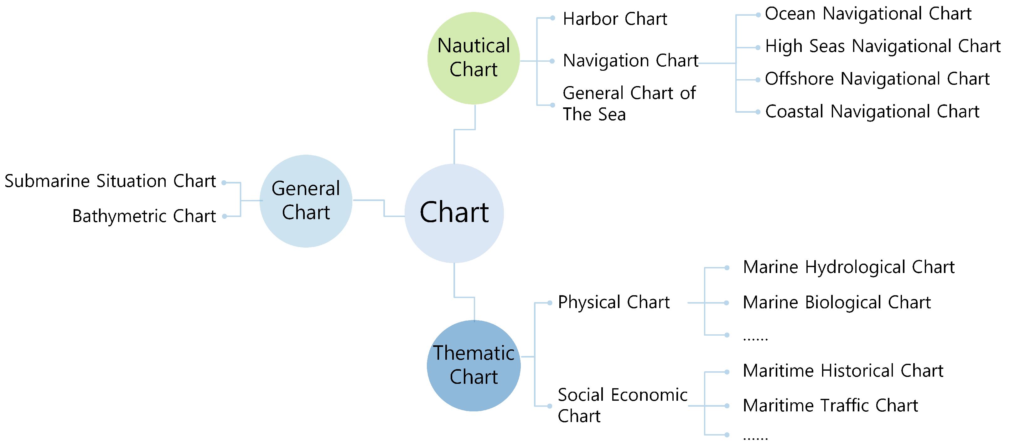
Figure 1. Types of charts.
Ijgi 14 00257 g001
Figure 2. Electronic chart generalization using different operators.
Ijgi 14 00257 g002
Figure 3. Simplification of depth contours.
Ijgi 14 00257 g003
Figure 4. Aggregation of depth contours.
Ijgi 14 00257 g004
Figure 5. Smoothing of depth contours.
Ijgi 14 00257 g005
Figure 6. Distribution of chart generalization operators and methods.
Ijgi 14 00257 g006
Figure 7. Traditional methods of chart generalization.
Ijgi 14 00257 g007
Figure 8. Process for generalization of soundings.
Ijgi 14 00257 g008
Figure 9. Selection from a large number of soundings in cartographic products.
Ijgi 14 00257 g009
Figure 10. 3D visualization of the Multibeam Echosounder.
Ijgi 14 00257 g010
Figure 11. Exaggeration of depth contours in compliance with the principle of “expansion of shallow water and reduction of deep water”.
Ijgi 14 00257 g011
Figure 12. Soundings, depth contours, and coastlines after mapping the “.000” format chart structure.
Ijgi 14 00257 g012
Figure 13. Framework for GNN-based generalization solutions for nautical charts.
Ijgi 14 00257 g013
Figure 14. Schematic diagram of GNN and CNN convolution operations.
Ijgi 14 00257 g014
Figure 15. GCN architecture for sounding generalization.
Ijgi 14 00257 g015
Figure 16. Graph structure visualization and label distribution statistics.
Ijgi 14 00257 g016
Figure 17. Training and validation loss with the learning rate schedule.
Ijgi 14 00257 g017
Figure 18. Trends of classification metrics over training epochs.
Ijgi 14 00257 g018
Figure 19. Visualization of overlap and generalization among multi-scale coastline data and model inference.
Ijgi 14 00257 g019
Table 1. Comparison of charts and general topographic maps.
AspectsChartsGeneral Topographic Maps
Mathematical FoundationUses geocentric systems (e.g., WGS-84/CGCS2000), with depth referenced to the lowest tidal level.Uses geocentric and projection systems (e.g., WGS-84, UTM), with elevation referenced to mean sea level.
Data SourceMarine survey.Terrestrial survey.
Representation ContentFocuses on navigation and hydrographic features: coasts, reefs, depths, aids to navigation, shipping lanes, etc.Focuses on land features: water systems, settlements, transport, terrain, soil and vegetation, and boundaries. Marine content is minimal.
Representation MethodsMainly uses Mercator projection; scale not fixed.Uses various projections, with fixed scales.
Symbol and EncodingCodes follow international standards (e.g., S-57).Codes based on national standards; symbols follow unified design rules.
Accuracy RequirementsHigh for position and depth, ensuring navigational safety.Varies by scale and terrain, focusing on landform accuracy.
CorrectionFrequently updated for safety.Longer revision cycles, fewer updates.
Table 2. Specific manifestations and limitations of the traditional generalization methods.
Traditional MethodsOperatorsAdvantages   Limitations of Traditional MethodsRelated Research
Delaunay TriangulationSelection Simplification Exaggeration Aggregation DisplacementEffectively maintain geographic element proximity. Construct uniqueness. Stability and clear hierarchical structure.Local optimization limitations. High computational complexity. Difficult to express dynamic information.Soundings [12,13,14,15,16,17]. Depth contours [18,19,20]. Coastlines [21,22]. Islands [23,24,25].
Voronoi DiagramSelection Simplification SmoothingCaptures neighbor relations. Supports density analysis. Enables pairwise combination.High computational complexity. Inadequate representation of dynamic information. Data redundancySoundings [14,25,26]. Depth contours [27]. Islands [28,29,30,31].
Douglas–Peucker AlgorithmSimplification Exaggeration Aggregation DisplacementReduction in data volume. Significant features retained. Cannot be used directly for 3D terrain simplification.Starting point dependency. Prone to topology errors. Sensitive to data distribution. Limited spatial contextDBM [32]. Depth contours [33,34,35]. Coastlines [22,36]. Islands [37].
Buffer MethodSelection Simplification Exaggeration Aggregation DisplacementReduces redundancy and noise. Easy to implement and compute.Parameter-dependent. Limited in dense areas. Poor with dynamic features. Inconsistent globally.Soundings [38]. Depth contours [35]. Coastlines [22,36]. Islands [39,40].
Rolling Circle ModelSelection Simplification DisplacementApplicable to directional constraints. Algorithm commonality.Parameter dependency. High computational complexity.Depth contours [9,41,42].
B-Spline Snake ModelSimplification Exaggeration Aggregation Displacement SmoothingHigh degree of automation. Highly adaptable.Parameter dependency. High computational complexity. Limited spatial context.Depth contours [43,44,45].
Table 3. Comparison of several GNNs.
ModelsApplicability ScenariosKey FeaturesAdvantagesLimitations
GCNNode classification. Graph classification. Link prediction.Weighted aggregation of node features and neighbor features based on spectral graph theory.Global information capture. Simple and efficient. Widely applicable. Low computational complexity.Consumes memory and graphics memory. No large graphs. Transductive learning only. No new nodes embedding.
Graph SAGELarge-scale graph. Dynamic graph.Sample a fixed number (order K) of neighbors, with flexible feature aggregation (mean, max, etc., LSTM).Overcoming GCN Memory and Graphics Limitations. Inductive Learning. Shared parameters. Incremental learning support. Supervised and unsupervised tasks support.No weighted graphs support. Equal neighbor weights. Unstable embeddings. High gradient variance.
GATNode classification. Graph classification. Heterogeneous graph analysis.Dynamically assigning importance weights to neighboring nodes based on attention mechanism.Flexible attention mechanism. Fast computation and parallel computation. Transductive learning and Inductive Learning support. Highly scalable.High parameter count. No dynamic graph handling. Limited efficiency of large-scale graphs.
GAEGraph embedding. Graph reconstruction. Link prediction.Auto-encoder framework for low-dimensional embeddings.Unsupervised learning. Highly capable of capturing graph structure. Flexible encoder choice.Sparse graph sensitivity. Poor performance in heterogeneous and dynamic graphs. Limited generation capability.
Graph TransformerNode classification. Graph prediction.Combining Transformer’s Global Attention with Graph Structure Embedding.Greater characterization capabilities. Capture of long-range dependencies. Graph data efficiency. Over-smoothing and over-squeezing mitigations.Weak local focus. Higher computational complexity. Large-scale data dependency.
Graph DiffusionWeakly connected graphs. Sparse graphs. Graph clustering. Homogeneous graphs.The original adjacency matrix is replaced by the sparsified graph diffusion matrix.Strong global information capture. Suitable for sparse and noisy graphs. Enhanced clustering.Reliance on the assumption of homogeneity. Insufficient support for complex graph structures. Diffusion matrix preprocessing is computationally inefficient.
Graph MambaDynamic graphs. Long-range dependency modeling. Spatio-temporal data predictionAn efficient graph learning model combining state space models and selective scanning mechanisms.Capturing long-range dependencies. Highly adaptable in non-sequential graph. Reduced memory consumption.Strong reliance on high-quality graph data.
Table 4. Comparison of several popular machine learning architectures.
ModelsKey FeaturesAdvantagesLimitationsApplications
GNNMessage passing Non-Euclidean space modeling Graph topology adaptationHandles non-Euclidean data. Captures complex relations. Supports semi-supervised learning.Requires graph input. High cost for large graphs.Social networks. Molecular modeling. Traffic prediction. Vector map learning.
CNNTranslation invariance Local receptive fields Parameter sharingEfficient and shift-invariant. Optimizes local patterns.Weak in global context. Sensitive to scale/rotation. Fixed input size.Image tasks. Object detection. Medical segmentation. Action recognition.
GANGenerative adversarial training Minimax gameRealistic image generation. Learns complex distributions.Unstable training. Mode collapse. Hard to evaluate.Image synthesis. Data augmentation. Text-to-image. Domain transfer.
TransformersSelf-attention Positional encoding Global modelingCaptures long-range context. Supports parallelism. Handles varied input length.High computation. Data hungry.NLP tasks. Speech recognition. Time series. Multimodal fusion.
Disclaimer/Publisher’s Note: The statements, opinions and data contained in all publications are solely those of the individual author(s) and contributor(s) and not of MDPI and/or the editor(s). MDPI and/or the editor(s) disclaim responsibility for any injury to people or property resulting from any ideas, methods, instructions or products referred to in the content.